Development of a Methodology for Probable ...

Development of a Methodology for Probable Maximum Precipitation Estimation over the American River Watershed Using the WRF Model By ELCIN TAN B.S. (Istanbul Technical University) 1999 M.S. (Istanbul Technical University) 2001 DISSERTATION Submitted in partial satisfaction of the requirements for the degree of DOCTOR OF PHILOSOPHY in CIVIL AND ENVIRONMENTAL ENGINEERING in the OFFICE OF GRADUATE STUDIES of the UNIVERSITY OF CALIFORNIA DAVIS Approved: _____________________________________ M. Levent Kavvas, Chair

_____________________________________ Timothy R. Ginn

_____________________________________ Fabian A. Bombardelli Committee in Charge 2010 -i-

UMI Number: 3404936

All rights reserved INFORMATION TO ALL USERS The quality of this reproduction is dependent upon the quality of the copy submitted. In the unlikely event that the author did not send a complete manuscript and there are missing pages, these will be noted. Also, if material had to be removed, a note will indicate the deletion.

UMI 3404936 Copyright 2010 by ProQuest LLC. All rights reserved. This edition of the work is protected against unauthorized copying under Title 17, United States Code.

ProQuest LLC 789 East Eisenhower Parkway P.O. Box 1346 Ann Arbor, MI 48106-1346

Elcin Tan March 2010 Civil and Environmental Engineering

Development of a Methodology for Probable Maximum Precipitation Estimation over the American River Watershed Using the WRF Model Abstract

A new physically-based methodology for probable maximum precipitation (PMP) estimation is developed over the American River Watershed (ARW) using the Weather Research and Forecast (WRF-ARW) model. A persistent moisture flux convergence pattern, called Pineapple Express, is analyzed for 42 historical extreme precipitation events, and it is found that Pineapple Express causes extreme precipitation over the basin of interest. An average correlation between moisture flux convergence and maximum precipitation is estimated as 0.71 for 42 events. The performance of the WRF model is verified for precipitation by means of calibration and independent validation of the model. The calibration procedure is performed only for the first ranked flood event 1997 case, whereas the WRF model is validated for 42 historical cases. Three nested model domains are set up with horizontal resolutions of 27 km, 9 km, and 3 km over the basin of interest. As a result of Chi-square goodness-of-fit tests, the hypothesis that “the WRF model can be used in the determination of PMP over the ARW for both areal average and point estimates” is accepted at the 5% level of significance. The sensitivities of model physics options on precipitation are determined using 28 microphysics, atmospheric boundary layer, and cumulus parameterization schemes combinations. It is concluded that the best triplet option is Thompson microphysics, Grell 3D ensemble cumulus, and YSU boundary layer (TGY), based on 42 historical cases, and this TGY triplet is used for all analyses of this research.

-ii-

Four techniques are proposed to evaluate physically possible maximum precipitation using the WRF: 1. Perturbations of atmospheric conditions; 2. Shift in atmospheric conditions; 3. Replacement of atmospheric conditions among historical events; and 4. Thermodynamically possible worst-case scenario creation. Moreover, climate change effect on precipitation is discussed by emphasizing temperature increase in order to determine the physically possible upper limits of precipitation due to climate change. The simulation results indicate that the meridional shift in atmospheric conditions is the optimum method to determine maximum precipitation in consideration of cost and efficiency. Finally, exceedance probability analyses of the model results of 42 historical extreme precipitation events demonstrate that the 72-hr basin averaged probable maximum precipitation is 21.72 inches for the exceedance probability of 0.5 percent. On the other hand, the current operational PMP estimation for the American River Watershed is 28.57 inches as published in the hydrometeorological report no. 59 and a previous PMP value was 31.48 inches as published in the hydrometeorological report no. 36. According to the exceedance probability analyses of this proposed method, the exceedance probabilities of these two estimations correspond to 0.036 percent and 0.011 percent, respectively.

-iii-

DEDICATION

I dedicate my dissertation to Mustafa Kemal ATATURK & to my entire family for happy times I always remember, especially to them who make my life beautiful, livable, and virtuous:

Great Mother Adalet Atakan Grand Mother Ceyhan Andic Grand Father Hayrettin Andic Grand Aunt

Gulgun Atakan

Grand Uncle Seyhan Atakan Aunt

Pinar Emiroglu

Uncle I

Ziya Emiroglu

Uncle II

Yavuz Tan

Uncle III

Cetin Tan

Cousin

Evrim Tan

Mother

Bahar Tan

Father

Ali Hasan Tan

My dedication to my father goes twice since he is the only person who continuously believes in me, especially for the times I even doubted myself.

-iv-

ACKNOWLEDGMENTS I have completed this dissertation under the supervision of Prof. M. Levent Kavvas to whom I am indebted for providing me all the opportunities during my studies and guiding me with a great deal of patience and devotion. Prof. Timothy R. Ginn and Asst. Prof. Fabian A. Bombardelli are not only acknowledged for serving in my dissertation and qualifying examination committees, but they are also gratefully appreciated for being an indestructible rooks in my life. Prof. Carlos Puente and Dr. Z.Q. Chen are acknowledged for serving in my qualifying examination. There are no words to express my deep gratitude to Prof. H. Nuzhet Dalfes for his sagacious mentorship during the last decade. I would also like to thank Assoc. Prof. Yurdanur Sezginer Unal and Dr. Baris Onol for their continuous support and encouragement. I would like to state my appreciation to the staff of the Aeronautics and Astronautics Faculty at Istanbul Technical University who made my life easier. I have been affiliated with the Department of Meteorological Engineering as a research assistant, with a partial financial support during my PhD as a part of the academician training program of Istanbul Technical University. The staff of the Department of Civil and Environmental Engineering at UCDavis including its Hydrologic Research Laboratory and its Amorocho Hydraulics Laboratory are also appreciated. I have been financially supported from several projects of California Department of Water Resources, US Bureau of Reclamation, NCAR and NASA. I would like to thank numerous people who share their knowledge with open source community especially for the WRF, NCL, and R. I am grateful to my inspirations: Inci Abla, Ulker Serifsoy, Prof. Istemi Unsal, Dr. Peter P. Sullivan, Prof. Fevzi Unal, Asst. Prof. Jeremy Pal, and Dr. Filippo Giorgi. I would not complete my doctorate studies without my friends who have been with me all the time, no matter what: Bilkay Gulacti, Violet Shu Xu, Aysegul Yelkenci Firat, Deniz Firat, Dr. Regine Scheder, Daniel Nover, Cindy Nover, Bulent Tutkun, Gulcan Ucar Tutkun, Hakan Bagci, Alexander Yuen, Gorkem Gunbas, Ulas Apak, Dr. Baris Caldag, Ines Meireles, Yasemin Yilmaz, Deniz Demirhan Bari, Tamir Kamai, Dr. Bayram Celik, Burak Yikilmaz, Yasemin Polat Yikilmaz, Maya Yikilmaz, Melike Gurbuz, Alya Gurbuz, Akin Gurbuz, Umit Yildiz, Sanjeev K. Jha, Kristin Eastman Reardon, Dr. Sevinc S. Sengor, Ahmet Faruk Ozturk, Baris Ozgun, Dr. Seyda Acar, Asst. Prof. Seda Ersus Bilek, and Kerem Alper. Finally, I owe thanks to those unnamed persons who made me realize how much I love science/engineering by discriminating against me, misjudging my capacity, pretending to help me, and saying things behind my back to destroy my career.

-v-

LIST of TABLES

Table 2.1 The WRF microphysics options (ARW-Version3) .......................................................27 Table 2.2 The WRF cumulus parameterization options (ARW-Version3) ................................32 Table 2.3 The WRF planetary boundary layer parameterization options (ARW-Version3) ...37 Table 3.1 The WRF model physics option configurations for calibration purposes ...............54 Table 3.2 72-hour maximum watershed averaged precipitation of the American River Watershed observation vs. the WRF model for validation purposes (USACE, 2005) ............55 Table 3.3 Precipitation observation stations ..................................................................................58 Table 3.4 Precipitation observations vs. the WRF precipitation (inches) ..................................59 Table 3.5 Station based Chi-square goodness-of-fit test ..............................................................61 Table 3.6 SET-I The WRF model physics option configurations- Sensitivity analyses of MP ........................................................................................................................................................63 Table 3.7 SET-II The WRF model physics option configurations- Sensitivity analyses of PBL .......................................................................................................................................................64 Table 3.8 SET-III The WRF model physics option configurations- Sensitivity analyses of CU ........................................................................................................................................................64 Table 4.1 The WRF model precipitation versus convergence term of MFC correlations .....88 Table 4.2 Minimum and maximum values of relative humidity and wind velocity for 42 extreme precipitation events during a 52-year historical period..................................................99 Table 4.3 Moisture and wind maximization combination effect on precipitation for the 1997 flood case ...........................................................................................................................................103 Table 4.4 IC only and combined IC+BC effects on precipitation based on wind maximization (1997 event only) .....................................................................................................104 Table 4.5 72-hr maximum basin averaged precipitation for replaced events (inches) ...........106 Table 4.6 72-hr maximum basin averaged precipitation obtained by meridional shifting (inches) ...............................................................................................................................................110 Table 4.7 72-hr maximum basin averaged precipitation obtained by meridional shifting for 42 historical events (inches) ..................................................................................................................112 Table 4.8 72-hr maximum basin averaged precipitation obtained by zonal shifting (inches) ...............................................................................................................................................113 Table 4.9 72-hr maximum basin averaged precipitation obtained by zonal shifting for all 42 historical events (inches) ..................................................................................................................115 Table 4.10 72-hr maximum basin-averaged precipitation under the saturated atmosphere (100% RH) conditions ....................................................................................................................117 -vi-

Table 4.11 Maximized precipitation for all 42 historical cases (inches) ...................................118 Table 4.12 72-hr maximum basin-averaged precipitable water (inches)...................................120 Table 4.13 Climate change effect on maximum precipitation based on the 1997 case .........122 Table 4.14 Precipitation maximization methods and their basin averaged values for the 1997 historical event (11.48 inches) .........................................................................................................124 Table 5.1 The validity of the main assumption of the traditional PMP methods .................130 Table 5.2 Statistical distributions and their parameters for historical events...........................148 Table 5.3 Precipitation for various degrees of exceedance probability (inches) ....................154 Table 6.1 Physically possible maximum Precipitation comparisons with Traditional PMP obtained from HMR59 (inches) .....................................................................................................158

-vii-

LIST of FIGURES

Figure 2.1 Horizontal and vertical grids of the WRF (ARW-Version3) ....................................24 Figure 2.2 The WRF-ARW model domain configuration............................................................43 Figure 3.1 GOES Visible 3:00 PM PST Tuesday Dec 31, 1996 .................................................47 Figure 3.2 The synoptic pattern of the 1997 event (NOAA, 1997) ...........................................48 Figure 3.3 300 mb wind vector climatology for December 26 - January 3 (1968-1996) (NOAA, 1997) ....................................................................................................................................48 Figure 3.4 300 mb wind vector analysis for the 1997 event (NOAA, 1997) .............................49 Figure 3.5 Composite mean precipitable water on January 1, 1997 (NOAA, 1997) ................50 Figure 3.6 Water vapor mixing ratio results of the WRF at Eta Level 11 on January 1, 1997 ......................................................................................................................................................50 Figure 3.7 The map of the American River Watershed and precipitation stations..................58 Figure 3.8 The WRF Physics option sensitivities to precipitation ..............................................66 Figure 4.1 Pineapple express events that caused extreme precipitation and flood ..................72 Figure 4.2 Pineapple express events that did not cause extreme precipitation and flood.......80 Figure 4.3 Pineapple express effect on maximum precipitation of January 97 ........................83 Figure 4.4 Horizontal moisture flux profiles for 42 historical cases ..........................................90 Figure 4.5 Maximum precipitation change with moisture only for the 1997 case .................100 Figure 4.6 Maximum precipitation change with wind speed only for the 1997 case .............102 Figure 4.7 Combined moisture and wind perturbation effect on precipitation for the 1997 flood case ...........................................................................................................................................103 Figure 4.8 IC only and combined IC+BC effects on precipitation for the 1997 case only ..105 Figure 4.9 The WRF precipitation results of replaced events ...................................................107 Figure 4.10 Meridionally shifted maximum precipitation (inches) ...........................................109 Figure 4.11 Zonally shifted maximum precipitation (inches) ....................................................113 Figure 4.12 72-hr maximum basin-averaged precipitation change with the increase in temperature ........................................................................................................................................122

Figure 5.1 Maximum observed point rainfalls as a function of duration. (Courtesy of John Vogel, National Weather Service [NRC94]) .................................................................................125

-viii-

Figure 5.2 Precipitable Water vs. Precipitation (inches)..............................................................128 Figure 5.3 Time series of the ratios of precipitation to precipitable water .............................131 Figure 5.4 Time series of the modeled and approximated PMP ..............................................131 Figure 5.5 Relative frequency histogram of 72-hr maximum basin averaged precipitation for the historical storms at the ARW ...................................................................................................133 Figure 5.6 Exceedance probability distribution of 72-hr maximum basin averaged precipitation for historical storms at the ARW ............................................................................133 Figure 5.7 Gamma distribution fitted to the relative frequency histogram of 72-hr maximum basin averaged precipitation for the historical storms at the ARW ..........................................134 Figure 5.8 Q-Q plot for historical storms at the ARW ..............................................................134 Figure 5.9 Relative frequency histogram of 72-hr maximum basin averaged precipitation for the historical storms at the ARW after a 2 degrees shift from N to S .....................................135 Figure 5.10 Exceedance probability distribution of 72-hr maximum basin averaged precipitation for historical storms at the ARW after a 2 degrees N to S shift ........................135 Figure 5.11 Gamma distribution fitted to the relative frequency histogram of 72-hr maximum basin averaged precipitation for the historical storms at the ARW after a 2 degrees N to S shift ........................................................................................................................................136 Figure 5.12 Q-Q plot for historical storms after a 2 degrees N to S shift ..............................136 Figure 5.13 Relative frequency histogram of 72-hr maximum basin averaged precipitation for the historical storms at the ARW after a 4 degrees shift from N to S .....................................137 Figure 5.14 Exceedance probability distribution of 72-hr maximum basin averaged precipitation for historical storms at the ARW after a 4 degrees N to S shift ........................137 Figure 5.15 Gamma distribution fitted to the relative frequency histogram of 72-hr maximum basin averaged precipitation for the historical storms at the ARW after a 4 degrees N to S shift ........................................................................................................................................138 Figure 5.16 Q-Q plot for historical storms after a 4 degrees N to S shift ..............................138 Figure 5.17 Relative frequency histogram of 72-hr maximum basin averaged precipitation for the historical storms at the ARW after a 6 degrees shift from N to S shift ............................139 Figure 5.18 Exceedance probability distribution of 72-hr maximum basin averaged precipitation for historical storms at the ARW after a 6 degrees N to S shift ........................139 Figure 5.19 Weibull distribution fitted to the relative frequency histogram of 72-hr maximum basin averaged precipitation for the historical storms at the ARW after a 6 degrees N to S shift .....................................................................................................................................................140 Figure 5.20 Q-Q plot for historical storms after a 6 degrees N to S shift ..............................140

-ix-

Figure 5.21 Relative frequency histogram of 72-hr maximum basin averaged precipitation for the historical storms at the ARW after a 6 degrees shift from W to E ....................................141 Figure 5.22 Exceedance probability distribution of 72-hr maximum basin averaged precipitation for historical storms at the ARW after a 6 degrees W to E shift ......................141 Figure 5.23 Gamma distribution fitted to the relative frequency histogram of 72-hr maximum basin averaged precipitation for the historical storms at the ARW after a 6 degrees W to E shift .......................................................................................................................................142 Figure 5.24 Q-Q plot for historical storms after a 6 degrees W to E shift .............................142 Figure 5.25 Relative frequency histogram of 72-hr maximum basin averaged precipitation for the historical storms at the ARW after a 100% relative humidity adjustment ........................143 Figure 5.26 Exceedance Probability Distribution of 72-hr maximum basin averaged precipitation for historical storms at the ARW after a 100% RH adjustment ........................143 Figure 5.27 Weibull distribution fitted to the relative frequency histogram of 72-hr maximum basin averaged precipitation for the historical storms at the ARW after a 100% RH adjustment .........................................................................................................................................144 Figure 5.28 Q-Q plot from historical storms after a 100% RH adjustment ...........................144 Figure 5.29 Relative frequency histogram of 72-hr maximum basin averaged precipitation for the historical storms at the ARW corresponding to the WRF model-calculated precipitable water....................................................................................................................................................145 Figure 5.30 Exceedance Probability Distribution of 72-hr maximum basin averaged precipitation for historical storms at the ARW corresponding to the WRF model-calculated precipitable water ..............................................................................................................................145 Figure 5.31 Gamma distribution fitted to the relative frequency histogram of 72-hr maximum basin averaged precipitation for the historical storms at the ARW corresponding to the WRF model-calculated precipitable water .........................................................................146 Figure 5.32 Q-Q plot from historical storms corresponding to precipitable water ..............146 Figure 5.33 Exceedance probability of the precipitation ratio- historical over 100% RH....151 Figure 5.34 Exceedance probability of the precipitation ratio- historical over PW ..............151 Figure 5.35 Exceedance probability of 72-hr maximum basin averaged precipitation for the historical storms at the ARW .........................................................................................................153 Figure 5.36 Exceedance probabilities of maximized historical events .....................................153

-x-

NOMENCLATURE

α d = 1 ρd

Specific volume for dry air

cp

Specific heat capacity at constant pressure

cs

Specific heat capacity of soil

cv

Specific heat capacity at constant volume

C

Convergence Influenced PMP

η

Vertical Coordinate Terrain Following Mass

φ = gz

Geopotential

F

Heat Flux

FU , FV , FW

Forcing terms of conservation of momentum

Fθ

Forcing term of conservation of energy

FQm

Forcing term of conservation of moisture

g

Gravitational Acceleration

γ = c p cv = 1.4

Ratio of the heat capacities

[1]

K

Empirically determined enveloping constant

[1]

K

Thermal diffusivity of soil

m = v, c, r,i, g, s

hydrometeors: water vapor, cloud vapor, rain, cloud ice, graupel, and snow, respectively.

µd = pdhs − pdht

Mass of dry air

ω = η

Contravariant Vertical Velocity

[1 kgm −3 ] ⎡⎣ J kg -1 K -1 ⎤⎦ ⎡⎣ J kg −1 K −1 ⎤⎦ ⎡⎣ J kg -1 K -1 ⎤⎦ [inches] [1] ⎡⎣ m 2s-2 ⎤⎦ ⎡⎣ W m −2 ⎤⎦

[N ] ⎡⎣ kg K s-1 ⎤⎦ ⎡⎣ kg 2 kg −1s −1 ⎤⎦ ⎡⎣ ms −2 ⎤⎦

⎡⎣ m 2 s −1 ⎤⎦

[mass per unit area]

-xi-

⎡⎣ m s-1 ⎤⎦

p

Pressure

[hPa]

p0

Reference Pressure

[hPa]

pdh

Hydrostatic component of the pressure for dry atmosphere

[hPa]

pdhs

Surface pdh

[hPa]

pdht

Top pdh

[hPa]

P

Precipitation

[inches]

Pmax

Maximum Precipitation

[inches]

PMP

Probable Maximum Precipitation

[inches]

PW =

1 p0 q dp ρw g ∫0

Precipitable Water

[kg m-2] or [in]

q

Specific Humidity

[kg kg-1]

q

Mixing Ratio

[mass per mass of dry air]

Q

Heating Rate

R = c p − cv

Gas Constant

⎡⎣ Ks-1 ⎤⎦ [J deg-1 kg-1]

Rd

Gas Constant for dry air

[J deg-1 kg-1]

ρs

Soil Density

⎡⎣ kg m −3 ⎤⎦

ρw

Density of water

⎡⎣ kg m −3 ⎤⎦

Sn ; σ

Standard Deviation

θ

Potential Temperature

[K]

T

Temperature

[K]

T

Total PMP

[inches]

v = ( u;v;w )

Covariant Velocities

⎡⎣ m s-1 ⎤⎦

-xii-

V = µd v = (U;V;W ) Velocities

⎡⎣ m s-1 ⎤⎦

w

Mixing Ratio

[kg kg-1]

wmax

Maximum Mixing Ratio

[kg kg-1]

X

Mean of the maximum observed daily precipitation

[inches]

Xmax

24-hr PMP

[inches]

-xiii-

ABBREVIATIONS

ACM2

Asymmetrical Convective Model Version 2

AFWA

Air Force Weather Agency

AMS

American Meteorological Society

AR

American River

ARs

Atmospheric Rivers

ARW

American River Watershed

ARW

Advanced Research WRF

BC

Boundary Condition

BMJ

Betts-Miller-Janjic CU scheme

CBL

Convective Boundary Layer

CAPE

Convective Available Potential Energy

CCDF

Complementart Cumulative Distribution Function

CDEC

California Data Exchange Center

CDF

Cumulative Distribution Function

CISL

Computational and Information Systems Laboratory at NCAR

CMBL

Cumulus, Microphysics and Boundary Layer

COMMAS

Collaborative Model for Multiscale Atmospheric Simulation

CU

Cumulus Parameterization

CV

Calibration and Validation

DAD

Depth-Area-Duration

DTC

Developmental Testbed Center

E

East direction

EGCP

Eta Grid-scale Cloud and Precipitation

ENSO

El-Nino Southern Oscillation

ETA

Eta Model

FAA

Federal Aviation Administration

FSL

Forecast Systems Laboratory

GCE

Goddard Cumulus Ensemble

GOES

Geostationary Operational Environmental Satellites

HMR36

Hydro-Meteorological Report No.36

HMR57

Hydro-Meteorological Report No.57

-xiv-

HMR58

Hydro-Meteorological Report No.58

HMR59

Hydro-Meteorological Report No.59

IC

Initial Condition

IPCC

Intergovernmental Panel on Climate Change

MFC

Moisture Flux Convergence

MJO

Madden Jullian Oscillation

MM5

PSU/NCAR mesoscale model

MMM

Mesoscale and Microscale Meteorology Division of NCAR

MOD

Model

MP

Maximum Precipitation

MP

Microphysics Parameterization

MPP

Maximum Possible Precipitation

MRF

Medium Range Forecast Model PBL

MYJ

Mellor-Yamada-Janjic PBL scheme

N

North direction

NCAR

National Center of Atmospheric Research

NCEP

National Centers for Environmental Prediction

NCL

NCAR Command Language

NH

Northern Hemipshere

NMM

Nonhydrostatic Mesoscale Model

NNRP

NCEP/NCAR Global Reanalysis Products

NOAA

National Oceanic and Atmospheric Administration

NRC

National Research Center

NS

PE shifting from the North to the South

NWP

Numerical Weather Prediction

OBS

Observation

OLR

Outgoing Longwave Radiation

PBL

Planetary Boundary Layer

PE

Pineapple Express

PEF

Possible Extreme Flood

PEP

Possible Extreme Precipitation

PMF

Probable Maximum Flood

PMP

Probable Maximum Precipitation

PNA

Pacific North American Pattern

-xv-

PNP

Persistent North Pacific Circulation

PRISM

Parameter-elevation Regressions on Independent Slopes Model Data

PSU

Penn State University

PW

Precipitable Water

QE

Qualifying Examination

QPF

Quantitative Precipitation Forecast

R

The Statistical Environment and Language R

RDA

Research Data Archive

RH

Relative Humidity

RRTM

Rapid Radiative Transfer Model

RUC

Rapid Update Cycle Model

S

South direction

STA

Statistic: Individual Scale Deviation Value

TGY

Thompson-Grell 3D-YSU scheme triplet

TKE

Turbulent Kinetic Energy

USACE

United States Army Corps of Engineers

USGS

United States Geological Survey

W

West direction

WE

PE shifting from the West to the East

WMO

World Meteorological Organization

WRF

Weather Research Forecast Model

WSF

The WRF Software Framework

WSM3

The WRF Single Moment 3-Class MP Scheme

WSM5

The WRF Single Moment 5-Class MP Scheme

WSM6

The WRF Single Moment 6-Class MP Scheme

WV

Water Vapor

YSU-PBL

Yonsei University PBL

-xvi-

TABLE of CONTENTS

Abstract..................................................................................................................................................... ii DEDICATION......................................................................................................................................... iv ACKNOWLEDGEMENTS......................................................................................................................v LIST of TABLES ..................................................................................................................................... vi LIST of FIGURES ................................................................................................................................. viii NOMENCLATURE ................................................................................................................................ xi ABBREVIATIONS ................................................................................................................................ xiv TABLE of CONTENTS ...................................................................................................................... xvii CHAPTER I- Introduction ....................................................................................................................... 1 1.1 Motivation ............................................................................................................................................. 1 1.2 Literature Review ................................................................................................................................. 2 1.3 Research Objectives ............................................................................................................................ 13 1.4 Methodology ....................................................................................................................................... 15 1.5 Scientific Value .................................................................................................................................... 16 1.6 Outline ................................................................................................................................................ 17 CHAPTER II- Methodology ................................................................................................................... 19 2.1 The Weather Research and Forecasting (WRF) model description ..................................................19 2.2 Cloud Microphysics Schemes ............................................................................................................ 26 2.2.1 Kessler scheme ........................................................................................................................... 27 2.2.2 Purdue Lin scheme ....................................................................................................................27 2.2.3 The WRF Single-Moment 3-class (WSM3) scheme ..................................................................28 2.2.4 The WRF Single-Moment 5-class (WSM5) scheme ..................................................................28 2.2.5 The WRF Single-Moment 6-class (WSM6) scheme ..................................................................29 2.2.6 Eta Grid-scale Cloud and Precipitation (2001) scheme- EGCP01.............................................29 2.2.7 Thompson et al. scheme ............................................................................................................29 2.2.8 Goddard Cumulus Ensemble Model (GCE) scheme ...............................................................30 2.2.9 Morrison scheme ....................................................................................................................... 31 2.3 Cumulus Parameterization ................................................................................................................. 31 2.3.1 Kain-Fritsch scheme .................................................................................................................. 32 2.3.2 Betts-Miller-Janjic scheme......................................................................................................... 33 2.3.3 Grell-Devenyi ensemble scheme ...............................................................................................33 2.3.4 Grell-3D ensemble scheme .......................................................................................................34 -xvii-

2.4 Planetary Boundary Layer (PBL) Parameterization ..........................................................................34 2.4.1 Medium Range Forecast Model (MRF) PBL ............................................................................37 2.4.2 Yonsei University (YSU) PBL ....................................................................................................37 2.4.3 Mellor-Yamada-Janjic (MYJ) PBL .............................................................................................38 2.4.4 Asymmetrical Convective Model Version 2 (Pleim) PBL-(ACM2) ...........................................38 2.5 Radiation Schemes ............................................................................................................................. 39 2.6 Land Surface Schemes ....................................................................................................................... 40 2.7 Model Configuration .......................................................................................................................... 42 Chapter III- Calibration and Validation of the WRF model with historical events ...............................44 3.1 Introduction ........................................................................................................................................ 44 3.2 Historical Events ................................................................................................................................ 44 3.2.1 Pineapple Express......................................................................................................................46 3.3 Data .................................................................................................................................................... 51 3.3.1 Model Data ................................................................................................................................. 51 3.3.2 Observation Data ....................................................................................................................... 51 3.4 Calibration and Validation .................................................................................................................52 3.5 Sensitivity Analysis ............................................................................................................................. 62 3.6 Chapter Conclusions .......................................................................................................................... 67 Chapter IV- Extreme Precipitation Estimation ......................................................................................69 4.1 Pineapple Express Effect ...................................................................................................................70 4.1.1 Direction, magnitude, and duration of the Pineapple Express ................................................81 4.2 Moisture Flux Convergence (MFC) ...................................................................................................84 4.2.1 Theory of MFC .......................................................................................................................... 84 4.2.2 Modeling of MFC ...................................................................................................................... 87 4.3 Precipitation Maximization Methods ................................................................................................97 4.3.1 Perturbations of Atmospheric Conditions ................................................................................98 4.3.1.1 Moisture Perturbation Effect ..........................................................................................98 4.3.1.2 Wind Perturbation Effect ..............................................................................................101 4.3.1.3 Combined Moisture and Wind Perturbation Effect .....................................................102 4.3.1.4 Perturbations in Initial and Boundary Conditions .......................................................104 4.3.2 Replacement of atmospheric conditions with respect to land conditions ..............................106 4.3.3 Shift in atmospheric conditions ...............................................................................................108 4.3.4 Thermodynamically possible worst-case scenario creation ....................................................116 4.4 Climate Change Effect on Precipitation of the American River Watershed....................................120

-xviii-

4.4.1 Effect of Temperature Change ...............................................................................................121 4.5 Chapter Conclusions ......................................................................................................................... 123 Chapter V- Results and Discussions ......................................................................................................125 Chapter VI- Summary and Conclusions ................................................................................................155 6.1 Future Perspectives ........................................................................................................................... 161 Appendix I .............................................................................................................................................. 162 Bibliography ........................................................................................................................................... 164

-xix-

1

CHAPTER I Introduction 1.1 Motivation To a society in a particular geographical region, dam failure is classified as one of many major potential hazards such as flood, levee failure, ground water recharge, disease transmission, fish survival that cause high losses, although their probability of occurrence is fairly low. According to the National Research Council (NRC), 26 percent of reported dam failures that occurred in the US between 1900 and 1979, are due to over-topping which represents about 13 percent of all incidents. The principal reason for over-topping is the inadequate spillway capacity for these incidents [NRC, 1983]. A spillway design is based on either the estimation of a probable maximum precipitation (PMP) directly, or the estimation of probable maximum flood (PMF) which is derived from PMP. Therefore, the accurate estimation of PMP plays a significant role in the design of dams and in dam failure reduction. There are several limitations in the current PMP methodology that reveal the need for a more accurate methodology. The original definition of PMP by the American Meteorological Society (AMS) was “the greatest depth of precipitation for a given duration meteorologically possible for a given basin at a particular time of year, with no allowance made for long-term climatic trends” [AMS, 1959]. This definition of PMP was changed in 1982 as “Theoretically, the greatest depth of precipitation for a given duration that is physically possible over a given size storm area at a particular geographical location at a certain time of year” [Hansen, 1987]. This revision in the PMP definition was “Due to the fact that knowledge of storm mechanisms and their precipitation-producing efficiency were

2 inadequate to permit precise evaluation of limiting values of extreme precipitation. Therefore PMP estimates were considered as approximations” [WMO, 1986]. PMP estimates are still considered as approximations [Corrigan et al., 1999 (HMR59, hereafter)] since they are still being used in operational hydrology as defined in 1982 although our knowledge about storm characteristics and their precipitation-producing efficiencies has advanced significantly in terms of making accurate assessments on extreme precipitation. The second limitation is that a PMP value needs to be updated each time a new major storm occurs since the PMP constants are determined with respect to the last big storm over a specified watershed. On the other hand, from its definition, PMP has been treated as a theoretical value that was not expected to occur. Hence, the current approach does not approximate an upper limit for the precipitation; it only estimates a precipitation value that is higher than what has occurred before. The third limitation, which is related to the first one, is that the current methodology is not physically based. This is emphasized in Hydro-Meteorological Report 57 as “while moisture is indeed maximized, numerous other factors are involved at a lesser level to effectively control unreasonable compounding of extremes” [Hansen et al., 1994 (HMR57, Hereafter)]. Other possible shortcomings of the traditional method are going to be discussed in the conclusion chapter. For these reasons, an operational and physically-based methodology that estimates an optimum PMP value, is needed to obtain accurate results that can supersede the current one. 1.2 Literature Review Operationally used Probable Maximum Precipitation (PMP) estimation methods can be classified according to their historical periods. Estimation of spillway design floods has

3 initially been performed according to the judgment of the design engineer. This period is called the early period [Myers, 1967]. Following period is the regional discharge period where design floods were determined based on Fuller’s work [Fuller, 1914], on area-related envelope formulae, and on statistical frequency analyses. The third period was called the storm transposition period, since design floods were calculated by using the storm transposition method [Myers, 1967]. Design flood studies have become popular since 1930’s with the increasing dam and levee constructions as an act of United States Government against the great economic depression. The PMP estimations were started soon after [Myers, 1967]. In this PMP period, the physical limiting factors on precipitation rate were classified to setup a method for PMP calculations as follows: humidity concentration that flows through the basin, wind rate that brings humidity to the basin, and water vapor (WV) that can be precipitated over the basin [Showalter and Solot, 1942]. In this dissertation, similar factors are going to be investigated for setting up a new method. The first limiting factor on precipitation, humidity that flows through the basin is associated with the maximum moisture in our study. Total specific humidity as a function of pressure in a unit atmospheric column, the so-called precipitable water (PW) is the best indicator for the evaluation of atmospheric moisture. During the time when PMP estimations started, precipitable water could not be calculated by direct measurements of specific humidity. So studies suggested estimating precipitable water using the surface dew point temperatures as a measure of atmospheric moisture content [Myers, 1967]. This approach to estimating PW was a very coarse approximation. Since we can measure and model atmospheric moisture content with current technology, there is no further need to make this assumption. Yet, this assumption is still being used in the current PMP method.

4 The second factor, the rate of wind that brings humidity to the basin is connected to wind maximization study of this dissertation. As we will discuss later, maximum wind speed and moisture are used to determine moisture flux convergence, which is a measure of precipitation. In traditional PMP studies, moisture convergence is neither calculated nor measured. Instead, being a coarse approximation, storm adjustment technique is used to take into account the convergence [Myers, 1967]. In this study, modeling of the maximum horizontal convergence is going to be proposed in order to obtain accurate estimations for PMP. The last limiting factor, the water vapor (WV) that can be precipitated over a basin, is nearly analogous to cumulus parameterization part of a numerical modeling approach. In the traditional method a quite primitive cloud model was developed by assuming that inflow occurs in the lower third of a cloud, outflow occurs in the upper third, and the middle third experiences only the associated vertical wind and moisture motion. Maximum height of the cloud was assumed to extend to the tropopause for the major storms. It was also assumed that the maximum cloud height increased with temperature. The precipitation was assumed to increase by about 9 percent for each 1C increase in temperature [Myers, 1967]. As will be mentioned later in the cumulus parameterization section of the model, inflows and outflows do not necessarily occur in the assumed levels. Moreover, there are several parameters that are not taken into account, such as updrafts and downdrafts. In the modeling approach presented here, quite sophisticated cloud models are used. Moreover, these cloud models are used for determining large-scale convective systems which are associated with the wet events in California (Mo and Higgins, 1998b) . For smaller scales, microphysical properties of clouds should be considered. None of the PMP procedures takes into account these processes. Therefore, the numerical weather prediction (NWP) modeling approach is

5 proposed to solve cloud physics in detail. The current PMP estimations for California are based on Hydrometeorological Report No.58 (HMR58) [Corrigan et al., 1998] and HMR59 that were superseded by Hydrometeorological Report No.36 (HMR36) [U.S. Weather Bureau, 1969; U.S. Weather Bureau, 1961] in 1998-1999. The main methodological difference between HMR59 and HMR36 is that the depth-area-duration (DAD) relations were determined based on stormbased relations in HMR59. Meanwhile, DADs were calculated by using a primitive massconservation model that was based on the physical limiting factors, as explained in the PMP period section [Myers, 1967]. The current operational PMP is estimated primarily from historical extreme storm events over a specified region and nearby states with similar climatic regimes. This approach requires that PMP estimates have to be updated when new major storms occur. In general there are four different types of precipitation: 1. Frontal, 2. Convective, 3. Orographic and 4. Tropical that need to be assessed for reliable PMP calculations rather than two precipitation types as in traditional PMP methods. Moreover, combinations of those all four types of precipitation need to be determined for the major storm occurrences for a specified region instead of isolated storm considerations. For conventional PMP estimates, California is divided into several regions in order to handle orographic influences, and the transposition of the storms is adjusted by appropriate orographic influence factors. Yet, the precipitation depth, duration, and area are dependent upon orographic influences, which should be considered as a part of the storm mechanism. Traditional PMP estimates have been separated as general and local PMP estimates. Precipitation from local storms was differentiated from general-storm rainfall. General-storm PMP estimates were developed using the storm separation or envelopment technique, which provides a way of moisture

6 maximization and transposing of storms by separating the dynamically forced precipitation from the orographically-forced precipitation. In these storms, precipitation is divided into convergence influenced (non-terrain) and orographic (terrain-influenced) components, which correspond to general storm PMP and local PMP estimates, respectively. The orographic component of the storm (T/C) is factorized by the ratio of total PMP (T) to convergence (C) influenced (general storm) PMP, where total PMP is determined from the 100-year, 24-hour storm maps of NOAA Atlas-2 [WMO, 1986; HMR58; HMR59]. Several studies have been conducted to improve the accuracy of the current operational method for various locations. It should be noted that the PMP results of a location may not be representative for any other location unless they both are affected from the same weather system. For instance, it was found that pseudoadabiatic assumption overestimates PMP by about 6.9% on average for Chicago area [Chen and Bradley, 2006], which needs to be evaluated further for California. On the other hand, it is important to note that the pseudoadabiatic assumption is misused in PMP studies. In atmospheric science, pseudoadiabatic assumption states that all condensed water is immediately removed from an air parcel. Such a process is adiabatic in the sense that the heating rate, Q = 0 , but the mass of water in the parcel is not constant [Bohren and Albrecht, 1998]. On the other hand, the pseudoadiabatic chart, which is also known as Skew-T Log-P diagram, is the graphical solution to the Poisson’s equation: ⎛p ⎞ θ =T⎜ 0⎟ ⎝ p⎠

R cp

(1.1)

For dry air, R = Rd = 287J deg −1 kg −1 and c p = 1004J deg −1 kg −1 ; therefore, R c p = 0.286 .

7 A graphical form of the Equation 1.1 can be written as, T = (const)θ p 0.286

(1.2)

In the pseudoadiabatic chart, Appendix I, each value of the potential temperature, θ , represents a dry adiabat which is defined by a straight line with a particular slope which passes through the point p = 0 and T = 0 [Wallace and Hobbs, 2006]. Similarly, pseudoadiabats, and saturation mixing ratio lines are added to pseudoadiabatic chart for saturated air. In the current operational PMP estimations, maximum precipitation is estimated using the formula,

Pmax =

wmax ×P w

(1.3)

where Pmax is probable maximum precipitation, P is observed rainfall, w is precipitable water, and wmax is the maximized precipitable water as given by the maximum 24-hour persisting dew points [Wiesner, 1970; Abbs, 1999]. Unfortunately, there is another misusage in the terminology in that wmax is not precipitable water but is a mixing ratio that is obtained from the maximum 24-hour persisting dew points using the pseudoadiabatic chart. On the other hand, w is obtained from the actual dew point using the same chart. Actually, precipitable water (PW) is defined as the vertical integration of specific humidity as a function of pressure,

8 PW =

1 p0 q dp ρw g ∫0

(1.4)

where specific humidity, q , can be interchangeably used with mixing ratio, w . From the above, it follows that the traditional method does not consider the moisture content of the whole atmospheric column. It only takes into account surface moisture content of the maximization of precipitation. In other words, the ratio of the surface mixing ratios do not necessarily equate to the ratios of precipitable water. As such, it is surprising that Chen and Bradley found that pseudoadiabatic assumption overestimates PMP [2006], since the maximization factor should be small when only surface moisture content is used. On the other hand, this might explain why PMP values are exceeded in some regions each time a new storm occurs and why these values are too high for some other regions. From another perspective, the maximum 24-hr persisting dew point temperature usage is also problematic, since the surface dew point temperature changes very dramatically with time, especially diurnally. Therefore, persisting dew point temperature assumption may not be valid. In the new method, presented here, these assumptions are eliminated, especially since atmospheric moisture tendencies are simulated in 3D. Other limitations of the current method may be addressed using the storm catalog method. One is that PMP is too high for Chicago area and the other is that the determination of the mean moisture availability is difficult if the storm has multiple rain periods. The most obvious constraint found in this study is that the moisture maximization method violates the physical rule since the dew temperature profile cannot be greater than the temperature profile [Chen and Bradley, 2007]. It is pointed out that no estimates of the PMP exist for small areas such as armored slopes, and for very short durations [Codell, 1986;

9 Hua et al., 2006]. For such cases one day PMP estimations are performed [Rakhecha and Clark, 1999]. It is shown that for short durations and small areas, PMP estimates are exceeded by 29% for Australian extraordinary short-duration heavy rainfall [Shepherd and Colquhoun, 1985]. In practice, the above-mentioned studies are valuable attempts for tuning the current method. They are also important indicators that the current PMP estimations need to be improved. However, the results of these estimations may never be as accurate as the results of the numerical atmospheric models. In addition to the operational storm-based and moisture convergence approaches there are several non-operational PMP estimation techniques that can be classified as i) statistical approach, and ii) numerical weather prediction modeling approach. Numerical Weather Modeling approach can be seen as an improvement to the moisture convergence approach, although it is not operational yet. The approach, proposed in this research, can be assessed as a combination of storm-based, moisture-convergence, and numerical weather prediction modeling approaches. In the statistical approach, one practice is to perform DAD analysis based on rainfall data [Morgan, 1914; Corps of Eng., 1945; Miami Con. Dist., 1936]. One can argue that this method does not work for the places with no rainfall data. Therefore, the users of this method apply extrapolation methods. Analogous to Fuller’s work [Myers, 1967], the “state-ofthe-art” practice is to calculate PMP based on a generalized frequency equation [Hershfield, 1961]: Xmax = X + KSn

(1.2)

10 Xmax is the 24-hr PMP at a given observing point; X is the mean of the maximum observed daily precipitation; Sn is the standard deviation of this time series; and the constant K is determined empirically by an enveloping process. Hershfield [1961] found K=15 for the United States based on 2645 station records. It should be noted that PMP is highly dependent upon location and therefore the 15 standard deviations may not be representative for some locations. There are numerous applications of the statistical approach for different locations [Campos-Aranda, 1998; Clark, 2002, 2003; Clark and Rakhecha, 2002; Clark, 1967; Desa and Rakhecha, 2007; Dhar and Kamte, 1969, 1971; Dhar and Nandargi, 1993a, 1993b; Dhar et al., 1981; Dhar et al., 1982; Ghahraman, 2008; Hansen, 1975; Jeevarathnam and Jayakumar, 1981; Nobilis et al., 1991; Rezacova et al., 2005] using different techniques [Casas et al., 2008; Douglas and Barros, 2003, 2004; Eliasson, 1997; Kennedy and Hart, 1984; Koutsoyiannis, 1999, 2004a, 2004b; Koutsoyiannis and Baloutsos, 2000]. There are also studies that used storm-based and moisture convergence approaches to determine PMP for different locations [Ding et al., 1986; Kennedy and Hart, 1984; Kulkarni and Nandargi, 1996; Leverson, 1986; Piper et al., 1994; Rakhecha and Kennedy, 1985; Rakhecha and Kulkarni, 1993; Rakhecha and Soman, 1994; Rakhecha and Clark, 2000; Rakhecha et al., 1992a, 1992b; Rakhecha et al., 1995a; Rakhecha et al., 1995b; Schreiner, 1978; Sharma et al., 1988; Singh et al., 1992; Svensson and Rakhecha, 1998; Thompson, 2003; Wang, 1984; Wiesner, 1970; Zhan and Zou, 1986; Zhan and Zhou, 1984]. Applications of numerical weather prediction models to PMP estimation are limited. MM5 was used for a heavy rainfall event that occurred in Kansas-Oklahoma border and it was suggested that the mesoscale models can be useful tools for the assessment of extreme rainfall producing storms in small areas and during short time periods [Zhao et al., 1997].

11 Four extreme events in Australia were modeled by using RAMS regional atmospheric model to investigate the assumptions used in the PMP estimations. It was suggested that despite the efficiencies found in that study, no operational replacement was possible for the current PMP [Abbs, 1999]. Another modeling-based methodology [Cotton et al., 2002] for determining extreme precipitation potential was performed for Colorado by using a convective-storm-resolving mesoscale model (RAMS). Although the precipitation amounts were obtained by the model for six extreme precipitation events, Hershfield’s (1965) PMP technique was used with some modifications [Cotton et al., 2002]. Chen [2005] also suggested that mesoscale models could be used in a limited way to improve traditional PMP results. The method, proposed in this research, is different than the mentioned previous efforts in that precipitation maximization techniques are developed using an atmospheric model. Traditional PMP calculations depending on geographical formation of a basin. On the other hand, the determination of the persistent weather systems and their interactions for specific locations is also crucial. Since our research is focused on the American River Watershed (ARW), we need to determine weather systems that cause extreme precipitation in this domain of interest. The identification of the extreme precipitation mechanisms for our domain requires much effort for several reasons, one of which is the scale problem that multiple timescales are involved in the system. 52 years of precipitation analysis was performed over the ARW. It was found that annual maximum precipitation occurs between October and April, which corresponds to the most active storm tracks in the North Pacific. Associated with extratropical cyclone activities [Rafael and Mills, 1996], major floods in California are caused by the “Pineapple Express” or atmospheric rivers (ARs), which describes a path of an extensive amount of moisture that traverses over Hawaiian Islands to enter California. This weather system is also called as TEREC, for “Truly Extraordinary

12 Rainfall Event in California“ [Baker and Estes, 1994]. These events might be associated with persistent atmospheric circulation anomaly patterns, one of which occurs in the North Pacific to the South of the Aleutians [Dole and Gordon, 1983]. The Pacific decadal timescale variations are linked to recent changes in frequency and intensity of El Niño versus La Niña events. It was also shown that the Aleutian Low pressure system, which is another important weather system in the pineapple express determination, shifts according to the decadal atmosphere-ocean variations [Trenberth and Hurrell, 1994]. Extreme precipitation events might also be related to a major teleconnection pattern, called Pacific North American pattern (PNA), which occurs in the Northern Hemisphere winter and is indicated by the midtropospheric geopotential height fields [Wallace and Gutzler, 1981]. Being a climate-scale phenomenon, El-Niño Southern Oscillation (ENSO) is connected to precipitation variability in North America [Ropelewski and Halpert, 1986; Schonher and Nicholson, 1989; Cayan and Peterson, 1989; Cayan and Redmond, 1994; Cayan et al., 1999; Kahya and Dracup, 1994; Mo and Higgins, 1998a; Dettinger et al., 1998]. It is shown that the extreme precipitation events occur at all phases of the ENSO cycle, but the largest fraction of these events occur during the neutral winters just prior to the onset of El-Niño [Higgins et al., 2000]. Moreover, it was shown that there is a link between persistent North Pacific (PNP) circulation anomalies and tropical interseasonal oscillations in Northern Hemisphere (NH) winter that might explain the extension in Pacific jet [Higgins and Mo, 1997]. This extension generally leads to the supply of extensive amount of moisture to the West coast of the U.S. On the other hand, fluctuations in the Pacific jet are associated with 28-72 day planetaryscale oscillations of outgoing longwave radiation OLR [Weickman et. al, 1985]. An association was found from the 36-40 day oscillatory modes of OLR [Mo, 1999] that California rainfall might be related to the 40-50 day oscillation, the so-called Madden-Jullian Oscillation (MJO),

13 that is the result of the orientation of the large-scale circulation cells eastwardly from Indian Ocean to the central Pacific. In addition, the tropical cyclone formation may be related to this oscillation [Nakazawa, 1986]. A possible mechanism may be the Ekman Pumping in the boundary layer, which may provide large-scale convergence for tropical cyclone occurrence [Madden and Julian, 1994]. Tropical influences on California precipitation are emphasized by heavy precipitation over California under the conditions that rainfall in the subtropical eastern Pacific is suppressed and convection in the central Pacific is enhanced [Mo and Higgins, 1998b]. On the other hand, no systematic relationship was found between annual variability in the amplitude of the MJO and the occurrence of the extreme events in California [Jones, 2000]. Controversially, the phase of the MJO has a substantial systematic effect on intraseasonal variability in precipitation in Oregon and Washington [Bond and Vecchi, 2003]. As will be shown in the next chapters, the extreme precipitation over Oregon, Washington, and California is a result of the same weather pattern. Therefore, MJO may have an effect on extreme precipitation over California. In conclusion, the current operational methodology is a quasi-deterministic procedure as mentioned by Dawdy and Lettenmaier [1987]. Accordingly, our goal is to develop a deterministic procedure in this sense. Moreover, the procedure, developed here, will accommodate stochastic components at the same time, since stochastic-dynamic methods may provide better solutions than fully deterministic approaches due to the capability of stochastic-dynamic methods estimating uncertainties (initial condition, observation, imperfect parameterization, etc) quantitatively [Joshi and Sikka, 1986]. 1.3 Research Objectives The main objective of this dissertation is to model physically possible maximum precipitation based on 42-year historical data, assuming no climate change effect included, to

14 be utilized in determining the appropriate cloud microphysics, cumulus, and planetary boundary layers parameterization schemes/packages of the Weather Research and Forecast (WRF-ARW) model for the American River Watershed (ARW). "The historical record of extreme events may not be representative of future frequencies of extreme events in the case where the processes governing extreme event occurrence change.  This may result from climate change if such occurs on the time scale of these observation collections" [T. R. Ginn, 2010, personal communication]. One of the aims of this dissertation is to show that the current probable maximum precipitation (PMP) estimations for AR are outdated and the current numerical weather prediction models can simulate PMP more accurately than the traditional method. Until now, PMP calculations have been performed by statistical methods in which physical phenomena were tabulated based on historical data by which those tables were updated with the occurrence of major storms. Those tables have been very useful for the time when physically based models could not be used. With the current modeling technology, although it may not be possible to obtain perfect results, it is possible to make improved estimations with certain confidence limits. The main research needs of this study are parallel to the needs of numerical atmospheric models concerning improvements in initial and boundary conditions (IC/BC) and in model physics. The physics of the models get weaker with the simulations of finer resolutions in order to obtain more spatial detail on atmosphere. The problem becomes more complex due to finer resolutions that are required to solve more unknowns dealing with detailed physics. Local factors become more significant when the problems need to be adapted to the combination of the effects with varying scales. For instance, at the most coarse resolution R15 (~4.5° × 7.5°), Parallel Climate Model [Barnett et al, 2004] resolves only two grid points

15 over California. This means that if one were to model precipitation, orography cannot be considered. On the other hand, a local model can only simulate precipitation due to orography. Several techniques exist [Federico, 2006] to overcome this scale problem in order to combine the effects related to different scales, but the main deficiencies are still the IC/ BC issues and model physics. 1.4 Methodology In order to determine probable maximum precipitation, a physically based deterministic modeling approach is proposed. Considering advantages and disadvantages of several atmospheric models, The Weather Research and Forecasting Model (WRF) model has been selected for PMP modeling due to the following reasons: 1. The WRF model incorporates advanced numeric and data assimilation techniques, a multiple relocatable nesting capability, and improved physics, particularly for treatment of convection and mesoscale precipitation. 2. It is intended for a wide range of applications, from idealized research to operational forecasting, with priority emphasis on horizontal grids of 1-10 kilometers. 3. The WRF interface is intended to be user friendly to allow easy exchange of packages with other models and/or to upgrade them. The WRF model is called one of the next generation models that some organizations combine with their own models. For instance, NCAR’s Mesoscale and Microscale Meteorology Division (MMM) is going to migrate its own research to the WRF which will replace NCAR/Pennsylvania State MM5 model. NOAA’s Forecast Systems Laboratory (FSL) will gradually transfer its development efforts from its RUC model to the WRF model.

16 NOAA’s National Centers for Environmental Prediction (NCEP) will implement the WRF model as a high-resolution nest within its operational regional forecast model (Eta) and will consider it as a replacement for its regional model [Rassmussen, 1999]. Using the WRF model and based on a 42 extreme event record, the best physical options for simulating extreme conditions more accurately will be determined first for the domain of interest. After this step of calibration and validation of the model, several maximization methods will be performed in order to determine a physical range for probable maximum precipitation. An upper limit for precipitation is expected to be determined so that one can make an interpretation for an optimum PMP distribution that is sought for the AR basin, the focus of this study. 1.5 Scientific Value The main contribution of this study is to develop a new methodology by which one can determine physically possible maximum precipitation values that will provide input to the civil engineering computations for the design and management of such structures as dams, levees, spillways and highways. Studies show that PMP values may be either too high which result in over-design, or too low resulting in excessive flood control costs depending on the location. For this reason, PMP values should be determined according to the location, and the strength of the proposed method is that the PMP can be evaluated accurately for any location even when there exist no observations. The usage of maximum precipitation values as initial and boundary conditions in flood simulation models would be another value of this dissertation, since they can help improve the accuracy of Probable Maximum Flood (PMF) estimations.

17 As a secondary scope of this dissertation, further contribution may be related to the quantitative precipitation forecasting (QPF) purposes, especially for the management of dam reservoirs to provide an early warning which can help to reduce the risk of flooding with emergency levee constructions. This work may also provide novel information on climate change related extreme events, whose importance is emphasized by IPCC as an announcement in the new special report on “Managing the Risks of Extreme Events and Disasters to Advance Climate Change Adaptation.” [IPCC, 2009]. Further climate change related contribution of this work may comprise coastal engineering applications that are closely related to eustatic sea level rise and precipitation whose change is projected by IPCC [2007] in terms of storm intensity and severity. 1.6 Outline In this first chapter, the motivation for introducing the concept of probable maximum precipitation, its calculation methods in literature and its importance in civil engineering applications is defined, emphasizing that the traditional method needs to be updated. The research objectives of this dissertation, focusing on the American River Watershed, are stated, and the mechanisms, which bring extreme precipitation over this domain of interest, are investigated. In the second chapter, the proposed method shall be introduced in more detail, and the physics behind it will be emphasized. The third chapter examines the applicability of the developed new method. The best physics options of the model shall be determined in terms of cumulus parameterization,

18 microphysics, and planetary boundary layer for the domain of interest, comparing basin averaged and point observations of precipitation. In the fourth chapter the maximization techniques of precipitation shall be elucidated, and shall be introduced as new probable maximum precipitation calculations. In the fifth chapter the results of application of the developed methodology shall be discussed in detail, comparing the results of the traditional and other methods proposed in the literature. In the sixth chapter the dissertation shall be concluded, stating the future goals after summarizing the application results and stating the conclusions on the proposed methodology.

19

CHAPTER II Methodology 2.1 The Weather Research and Forecasting (WRF) model description The Weather Research and Forecast Model (WRF) [Skamarock et al., 2008], called the next generation numerical weather prediction system, has been developed with the partnership of NCAR, the National Oceanic and Atmospheric Administration (the National Centers for Environmental Prediction (NCEP) and the Forecast Systems Laboratory (FSL)), the Air Force Weather Agency (AFWA), the Naval Research Laboratory, Oklahoma University, and the Federal Aviation Administration (FAA). The replacement of the models of those organizations (MM5, RUC, ETA) with the WRF has been gradually started. The current WRF (Weather Research and Forecasting Model) software framework (WSF) supports two dynamical solvers: the Advanced Research WRF (WRF-ARW) that is used in this research, developed and maintained by the Mesoscale and Microscale Meteorology Division of NCAR, and the nonhydrostatic Mesoscale Model (NMM) developed by the National Centers for Environmental Prediction with user support provided by the Developmental Testbed Center (www.wrf-model.org). The equations in this sub-section are summarized from the Advanced Research WRF Description-Version3 [Skamarock et al., 2008]. The WRF is a Eulerian, nonhydrostatic, fully compressible, scalar variable conserved three-dimensional primitive equation model. The prognostic equations for each variable (wind, potential temperature, moisture and hydrometeor fields) are formulated in flux form using a terrain-following mass vertical coordinate denoted by η and defined as,

20

η = ( pdh − pdht ) µd

(2.1)

µd = pdhs − pdht

(2.2)

where mass of dry air, µd , is

pdh denotes the hydrostatic component of the pressure for dry atmosphere, pdhs and pdht refer to values along the surface and top boundaries, respectively [Laprise, 1992]. η varies from a value of 1 at the surface to 0 at the top boundary of the model domain. The flux form of moist Euler equations in mass vertical coordinate can be written as, Conservation of momentum in x: ∂tU + [ ∇ ⋅ (Vu)] + µdα∂ x p + (α α d ) ∂η p∂ xφ = FU

(2.3)

Conservation of momentum in y: ∂tV + ⎡⎣∇ ⋅ ( Vv ) ⎤⎦ + µdα∂ y p + (α α d ) ∂η p∂ yφ = FV

(2.4)

Conservation of momentum in η :

∂tW + ⎡⎣∇ ⋅ ( Vw ) ⎤⎦ − g ⎡⎣(α α d ) ∂η p − µd ⎤⎦ = FW

(2.5)

where ∇ ⋅ (Vu) , ∇ ⋅ (Vv) , and ∇ ⋅ (Vw) are the flux forms of mass divergence in a terrain following coordinate for x, y, and η directions, respectively.

21 Conservation of energy (Thermodynamic Energy equation): ∂Θ + ( ∇ ⋅ Vθ ) = Fθ

(2.6)

Conservation of mass (Continuity equation): ∂t µ d + ( ∇ ⋅ V ) = 0

(2.7)

∂tφ + µd−1 ⎡⎣( V ⋅ ∇φ ) − gW ⎤⎦ = 0

(2.8)

Change in Geopotential:

Conservation of Water: ∂t Qm + ( ∇ ⋅ Vqm ) = FQm

(2.9)

along with the diagnostic relation for the specific volume for dry air is α d = 1 ρd , and

(

specific volume for moist air is α = α d 1 + qv + qc + qr + qi + qg + qs

)

−1

Qm = µd qm

(2.10)

qm = qv , qc , qr , qi , qg , qs

(2.11)

where qm is the mixing ratio (mass per mass of dry air) for water vapor, cloud water, rain, ice, graupel, and snow, respectively.

22 ∂ηφ = −α d µd

(2.12)

and equation of state, p = p0 ( Rdθ m p0α d )

(2.13)

θ m = θ (1 + ( Rv Rd ) qv ) ≈ θ (1 + 1.61qv )

(2.14)

γ

where

The subscripts x , y , and η denote differentiation; γ = c p cv = 1.4 is the ratio of the heat capacities at constant pressure and volume, for dry air. Rd is the gas constant for dry air, p0 is a reference pressure. FU , FV , FW , Fθ , and FQm represent forcing terms arising from model physics, turbulent mixing, spherical projections, and the rotation of the Earth. θ is the potential temperature, and non-conserved variables are the geopotential, φ = gz and the pressure, p . Since µd ( x, y ) is the mass per unit area within the column in the model domain, flux form of the variables are, V = µd v = (U;V;W )

(2.15)

Ω = µdη

(2.16)

Θ = µdθ

(2.17)

23 where v = ( u;v;w ) are the covariant velocities, which are the velocities of a cartesian coordinate system transformation, while ω = η is the contravariant vertical velocity, which is a vertical velocity of the inverse of that cartesian coordinate system transformation. For temporal discretization diverse time-integration schemes are used. The WRF-ARW solver uses a third-order Runge-Kutta (RK3) time integration scheme [Wicker and Skamarock, 2002]. Forward-backward time integration scheme is used for both horizontally propagating acoustic modes and gravity waves. The integrations of buoyancy oscillations and vertically propagating acoustic modes are integrated by a vertically implicit scheme over smaller time steps to maintain numerical stability. For spatial discretization, The WRF-ARW solver uses Arakawa-C horizontal grid staggered scheme [Arakawa and Lamb, 1977]. In the vertical direction, variables are defined with wind/mass fields on half η layers and the vertical velocity and TKE at the full layers.

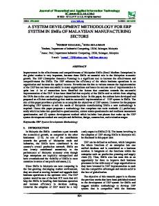
The WRF has downscaling/upscaling capabilities and many modeling options for various atmospheric processes. The WRF itself includes terrain elevation, land cover and land use data sets from USGS at various resolutions that cover the whole globe. The finest resolution of these data sets is 30 seconds in both latitudinal and longitudinal directions, which corresponds to about 1 km in length in mid-latitudes. The WRF uses ordinary Cartesian grids in the horizontal directions and a terrainfollowing η coordinate in the vertical direction. As a function of pressure, a dimensionless quantity eta is used to define the vertical levels between zero and one corresponding to the top and bottom of the troposphere, respectively. One may choose ten to forty vertical levels

24 which are not necessarily equally spaced. In the WRF, C type staggering [Arakawa and Lamb, 1977] is used for the calculation of the variables on grid cells for two horizontal dimensions that state variables/scalars (temperature, pressure and specific humidity) are computed at the middle of the grid cells shown as θ in Figure 2.1 while the horizontal velocity components are simulated at the half distance of the nodes of these grid cells. The advantage of C type staggering is that convergence and pressure terms are simulated in one unit distance only, which doubles the resolution of A type staggering. Thus geostrophic adjustment is calculated with improved accuracy. On the other hand, C staggering might be disadvantageous for inertia-gravity wave simulations [Kalnay, 2003]. In vertical, state variables are defined at the middle of the each eta level, while vertical velocity is computed at the eta levels. The WRF model is globally re-locatable with three map projections: Polar stereographic, Lambert conformal and Mercator. The map projections support different true latitudes for Lambert conformal projection, which we use for our domain of interest.

Figure 2.1 Horizontal and vertical grids of the WRF (ARW-Version3)

25 The model grid sizes are flexible and it has multiple nesting capabilities so that multiple domains (three nested domains are used in this study) could be run in the WRF, simultaneously. Each domain takes information from its parent domain at every time-step, and runs three time steps for each parent step before feeding back information to the parent domain on the coincident interior points. The feedback distinguishes two-way nesting from one-way nesting, and allows the nests to affect the coarse mesh solution, leading to better behavior at outflow boundaries. However there is significant overhead cost associated with the boundary interpolation and feedback at every time step. Due to the fact that the sub-grid scale processes are not simulated explicitly, they need to be somehow adjusted so that their significant influence on larger scales can be represented accurately. These adjustments are called parameterizations that are mainly applied to boundary layer, cloud, hydrological, radiation/chemical and ocean/land processes, in regional mesoscale models [Arakawa, 1997]. Reynolds averaging method is applied to handle both low and high-resolution effects where resolved processes are determined by grid-box averages whereas perturbations need to be parameterized. It is important to note at this point that it is also possible to solve those five main processes explicitly, including the necessary closure assumptions. They may even provide better representations than parameterization techniques, but the results of such an approach still do not compensate the cost and efficiency, although computers are getting extremely powerful. The WRF model has a wide range of physical process routines such as those handling advection, diffusion, radiation, planetary boundary layer, land surface, cumulus parameterization and cloud microphysics. In this research, we only focus on the options of cumulus parameterization, cloud microphysics and boundary layer physics for precipitation sensitivity analysis purposes.

26 2.2 Cloud Microphysics Schemes The parameterization of hydrological and chemical processes depends on the definition of source-sink terms in their prognostic equations. Regarding hydrological processes, three prognostic equations, called conservation of water equations, are added to the governing equations with three additional unknowns in specific humidity values for different phases of water. Freezing, deposition, condensation, and conversions of the phase changes are parameterized as source-sink terms for the closures. Cloud microphysics parameterization is handled by either using bin or bulk microphysics schemes in numerical weather prediction models. Bin (spectral) microphysics schemes that simulate the size spectra of liquid and ice particles are computationally more expensive than the bulk schemes, which have very simplified parameterizations especially when one moment of the particle size distribution is predicted [Lynn and Khain, 2007]. All microphysics parameterization options of the WRF are bulk schemes that are called two-moment schemes if they predict both mass and number densities. Cloud microphysics schemes resolve precipitation processes depending upon grid-scale saturation. Assuming that grid boxes are uniform, these processes are activated whenever the saturation is reached. Ice phase inclusion regarding graupel or hail depends on microphysics scheme. Temperature tendencies, all moist variables, and non-convective surface rainfalls are the outputs of those microphysical processes. They also provide cloud information to radiation schemes. All nine microphysics options of the WRF, shown in Table 2.1, are evaluated in this study for sensitivity analysis purposes.

27 Table 2.1 The WRF microphysics options (ARW-Version3) Number of Mixed Phase Scheme Ice-Phase Processes Variables Processes Kessler 3 No No Purdue Lin 6 Yes Yes WSM3 3 Yes No WSM5 5 Yes No WSM6 6 Yes Yes Eta GCP 2 Yes Yes Thompson 7 Yes Yes Goddard 6 Yes Yes Morrison 2-Moment 10 Yes Yes 2.2.1 Kessler scheme Kessler scheme, adapted from COMMAS [Wicker and Wilhelmson, 1995] model, is a simple warm cloud scheme where cloud water and rain fields are predicted explicitly with microphysical processes without any ice phase processes. These microphysical processes are the production, fall, and evaporation of rain; the accretion and auto-conversion of cloud water; and the production of cloud water from condensation [Kessler, 1969 (K69, hereafter)]. 2.2.2 Purdue Lin scheme Six classes of hydrometeors are included: water vapor, cloud water, rain, cloud ice, snow, and graupel. Production terms simulated for snow are ice crystal aggregation, accretion of cloud ice by snow, accretion of cloud water by snow, accretion of cloud ice by rain, accretion of rain by cloud ice particles, accretion of rain for snow, accretion of snow for rain, accretion of snow by hail/graupel, depositional growth of snow, melting of snow to from rain, cloud water transformation to snow by deposition, cloud ice transformation to snow by riming. Production terms calculated for hail/graupel are aggregation of cloud ice to form snow, accretion of cloud water by hail, accretion of cloud ice by hail, accretion of rain by hail, wet growth of hail, raindrop freezing, sublimation of hail, melting of hail. Production terms for rain are, auto-conversion of cloud droplets, accretion of cloud water by rain,

28 freezing of raindrops, melting of raindrops, evaporation of rain [Lin et al., 1983; Rutledge and Hobbs, 1984 (RH84)] Heat exchange and phase change of water substance are iteratively balanced in saturation adjustment part of the scheme with the inclusion of ice phase change [Tao et al., 1989]. 2.2.3 The WRF Single-Moment 3-class (WSM3) scheme WSM3 is a simple-ice scheme, adopted from Dudhia, 1989 [D89] which is also a continuation of Hsie scheme and Rutledge and Hobbs ([1983], (RH83)), that predicts vapor, cloud water or ice, and rain or snow, using three arrays. Cloud water and rain processes are taken into account when temperatures are above the temperature of freezing, while temperatures are either equal to or below the freezing temperature when the same arrays are treated for cloud ice and snow calculations. Cloud ice number concentrations are diagnosed from their mixing ratio. Intercept parameter for snow is temperature dependent, ice number concentrations are cloud-ice-mass dependent, and ice processes and auto-conversion of cloud water to rain are slightly different from D89 and RH83. Sedimentation of ice crystal is added to the scheme [Hong et al., 2004]. This scheme does not take into account super-cooled water processes and gradual melting rates of snow. Therefore, it is not a mixed phase scheme. 2.2.4 The WRF Single-Moment 5-class (WSM5) scheme WSM5 differs from WSM3 in that five hydrometeors (water vapor, rain, snow, cloud ice, and cloud water) are computed in their own arrays [Hong et al., 2004; Hong and Lim, 2006]. WSM5 is a mixed phase scheme where supercooled water processes and gradual melting rates of snow are simulated.

29 2.2.5 The WRF Single-Moment 6-class (WSM6) scheme The six-class scheme is similar to WSM5 scheme except that graupel is included as the sixth hydrometeor. Regarding to graupel-related terms, it is similar to Purdue-Lin scheme and RH84, although its ice-phase behavior is similar to WSM family schemes [Hong et al., 2004]. Terminal velocity, in other words fall speed of snow and graupel, is unified by its mass weighted average. Accretion rates of ice, cloud water and rain are modified according to their new terminal velocities with the elimination of snow-graupel accretion [Dudhia et al., 2008]. For a low-resolution grid (i.e, greater than 10km), WSM family schemes simulate precipitation similarly, although WSM6 simulates precipitation better for high-resolution grids (i.e., less than 10km) [Hong and Lim, 2006]. 2.2.6 Eta Grid-scale Cloud and Precipitation (2001) scheme- EGCP01 EGCP01, known also as Eta Ferrier, is a mixed-phase and six-class scheme. It assumes that the size distribution of precipitating ice is a function of temperature [Ryan, 1996]. Lookup tables are used for rain, precipitating ice and fall speed of rimed ice, which is a function of rime density. The gradual sedimentation of ice particles from upper levels is taken into account. Total condensation of cloud water, rain, and ice and their fractions are predicted in this scheme. Ice is categorized as small ice crystals, snow, graupel, and sleet. 2.2.7 Thompson et al. scheme Thompson scheme, which is also a bulk parameterization, can be classified as the most sophisticated one among the WRF microphysics. It is an upgrade version of Reisner et al. [1998] and Thompson et al. [2004]. The last Thompson scheme (The WRF-ARW V3.1.1) has also new modifications such as two-moment implication that is not mentioned in Thompson et al. [2008] [G. Thompson, 2009, personal communication]. The sum of exponential and

30 gamma distributions is used to describe snow size distribution which depends on both ice water content and temperature. Unlike any other microphysics schemes, snow is assumed to be non-spherical and its density varies inversely with diameter that is very close to observations. A threshold size of ice crystals are arbitrarily determined for the process of depositional growth onto cloud ice particles, so that slowly falling tiny ice crystals coexist with more rapidly falling snow. Regarding riming process, this scheme uses a variable collection efficiency based on volume diameter of snow and cloud water [Wang and Ji, 2000], rather than a constant used by other schemes. Constants that are used to calculate terminal velocities of snow, are matched to vertically pointing Doppler radar data. 2.2.8 Goddard Cumulus Ensemble Model (GCE) scheme The GCE [Tao and Simpson, 1993] is a one-moment bulk microphysical scheme where cloud water and rain are parameterized by K69 and the parameterization of cloud ice, snow, and hail/graupel is mainly based on Lin et al. [1983] with additional processes from RH84. The third class of ice can be chosen either as graupel or hail, whereas only two classes of ice can be simulated with the options of ice and graupel or ice and snow [McCumber et al., 1991]. A new saturation technique, designed to ensure that super saturation (sub-saturation) cannot exist at a grid point that is clear (cloudy), was added [Tao et. al., 1993; Tao et al., 2003]. There is also a control subroutine for conservation of water budget. 2.2.9 Morrison Scheme The Morrison scheme is a two-moment bulk microphysics scheme that is based on Morrison et al. [2005] and Morrison and Pinto [2006]. In this scheme, mass mixing ratios and number concentrations of five hydrometeor species; cloud droplets, cloud ice, snow, rain, and graupel, are predicted. The cloud and precipitation particle size distributions are

31 represented by gamma functions. Intercept and slope parameters of this distribution are derived from the predicted number concentrations, mixing ratio, and shape parameter for each species. All particles are assumed to be spheres and bulk particle densities of Reisner et al. [1998] are used. For the precipitation species shape parameter is selected as 0, so that size distributions of these species are exponential functions similar to Marshall-Pallmer distributions [Morrison et al., 2009]. 2.3 Cumulus Parameterization The parameterization of the cloud process, the so-called cumulus parameterization, is seen as one of the most complex problems in numerical weather prediction models. The main goal of cumulus parameterization is to represent the collective effect of the sub-grid scale clouds, which cannot be resolved explicitly. Cumulus parameterization schemes are based on the determination of the effects of cumulus convection in sub-grid scale regarding condensation in the updraft, evaporation in the downdraft, cooling due to the evaporation of falling rain below the cloud base, turbulent mixing at the cloud edge with the environment, entrainment, detrainment, and subsidence compensation in the boundary layer. They resolve sub-grid scale vertical fluxes and rainfall due to convective clouds. They produce columnar moisture, temperature tendencies and surface convective rainfall. Some cumulus parameterization schemes also produce columnar cloud tendencies. If the grid is fine enough (i.e., less than 5 km) to resolve updrafts and downdrafts then there is no need to use cumulus scheme. Convective adjustment technique is another way to resolve the vertical structure of the atmospheric column without simulating the explicit convective processes [Frank and Molinari, 1993]. In this technique, temperature and moisture is first predicted for a time step at each model grid neglecting condensation and development of any unstable lapse rates. Then the

32 vertical profiles of temperature and moisture at each grid point are examined for super adiabatic lapse rates and/or super saturation. In the unsaturated case, if the lapse rate exceeds the dry adiabatic value, it is restored to this value. If the air is saturated, and the calculated lapse rate exceeds the moist adiabatic lapse rate, then any excess moisture in the model grid must be condensed isobarically with the latent heat warming the air. Therefore, the temperature and the specific humidity are adjusted to bring the air in the model grid to a saturated state. This way, the model can compute precipitation through the computation of condensation at each model grid. Table 2.2 The WRF cumulus parameterization options (ARW-Version3) Scheme Kain-Fritsch Betts-Miller-Janjic Grell-Devenyi Grell-3D

Cloud Detrainment Yes No Yes Yes

Type Mass Flux Adjustment Mass Flux Mass Flux

Closure CAPE Removal Sounding Adjustment Various Various

2.3.1 Kain-Fritsch scheme Kain-Fritch, a complex cloud-mixing scheme [Kain, 2004], is the modification of FritschChappell type schemes [Kain and Fritsch, 1990; Kain and Fritsch, 1993). It determines updraft and downdraft properties with releasing convective available potential energy (CAPE), the maximum work done by buoyancy, given time scale. It is a mass flux type scheme and it can detrain cloud and precipitation in addition to vapor. The minimum entrainment rate is defined as 50% of the maximum possible entrainment rate to suppress convective initiation for unstable and dry environments. Maximum possible entrainment rate is controlled by cloud radius. Therefore, this radius is modified to alter as a function of sub-layer convergence [Frank and Cohen, 1987]. Deep convection activation is suppressed in weakly convergent or divergent environments, while it is enhanced in strongly convergent regimes.

33 The other necessary term for deep convection activation, minimum cloud depth, is a function of cloud-base temperature in this scheme rather than a constant as in its other versions. This modification helps to improve deep convection activation in shallow clouds, especially when ice-phase processes are active. In the conditions when minimum cloud depth cannot be adequate for deep convection, the scheme allows the formation of the nonprecipitating clouds. CAPE removal is used for the closure assumption where CAPE is based on the path of an ascending parcel with dilution. 2.3.2 Betts-Miller-Janjic scheme The Betts-Miller-Janjic (BMJ) scheme [Janjic, 1994; Janjic, 2000] is a modified version of the Betts-Miller (BM) convective adjustment scheme [Betts, 1986; Betts and Miller, 1986]. The major modification is related to the characterization of the deep convection regimes where the parameters used in moisture profile and relaxation time are switched to variables that are dependent upon a new parameter called cloud efficiency which is a function of mean cloud temperature, precipitation, and entropy change [Janjic, 1994]. For shallow convection moisture profile, a constraint is added to ensure that entropy change needs to be small and nonnegative. In this scheme there are two layers over the oceans. One is a viscous layer where the molecular diffusion is the driving mechanism for the vertical transport. The other is a layer above the viscous layer where turbulence is responsible for the vertical transport. 2.3.3 Grell-Devenyi ensemble scheme Grell-Devenyi scheme is based on a convective parameterization scheme developed by Grell [1993]. In Grell scheme clouds are pictured as two steady-state circulations, caused by an updraft and a downdraft. There is no direct mixing between cloud air and environmental air, except at the top and the bottom of the circulations. Cloud mass flux is constant with

34 height, and there is no entrainment or detrainment along the cloud edges. Therefore, the updraft and downdraft mass fluxes at their originating levels represent the mass fluxes through all the layers of a cloud. The main state variable of this scheme is the upward mass flux at the cloud base. It is determined from the buoyant energy, which is a function of the change in buoyant energy due to convection and the change in buoyant energy due to largescale destabilization. Finally, the rainfall is computed from a relation of water condensation in updraft, upward mass flux at the cloud base and precipitation efficiency [Fritsch and Chappell, 1980]. On the other hand, Grell-Devenyi scheme introduces a new convective parameterization framework where a large ensemble of assumptions used in Grell scheme is computed and the optimal value is given to the three-dimensional model as a weighted average. Parameterization ensembles that have at least 144 members are classified as dynamic control, feedback, and static control. Dynamic control shows the modulation of the convection by the environment, called feedback, and static control is the cloud model that is used to determine cloud properties [Grell and Devenyi, 2002]. 2.3.4 Grell-3D ensemble scheme This scheme is based on the ensemble mean convective parameterization approach as introduced in Grell and Devenyi scheme. In Grell-3D, quasi-equilibrium approach is not applied to the ensemble members. Subsidence effects are extended to the neighboring columns so that the scheme is more accurate for grid sizes less than 10km. 2.4 Planetary Boundary Layer (PBL) Parameterization There are a number of formulations for turbulent mixing and filtering available in the WRF solver. Some of them are used for numerical reasons, and other filters are designed to represent physical sub-grid turbulence processes. The ARW solver allows sub-grid scale

35 turbulence to be parameterized as it is treated in cloud-scale models including horizontal mixing.

However, when a PBL scheme is used, all other cloud-scale vertical mixing is

disabled, and vertical mixing is parameterized in the chosen PBL scheme. [Skamarock et al., 2008; Laprise,1992]. Planetary Boundary Layer schemes represent sub-grid vertical fluxes due to turbulence, and they are mostly distinguished by the treatment of the unstable boundary layer, providing columnar tendencies of heat, momentum and moisture. PBL schemes may also provide cloud tendencies and frictional effects on momentum. They are subdivided as surface layer, boundary layer and free atmosphere, and they have interaction with fluxes from surface layer and land-surface schemes. These one-dimensional schemes assume a clear separation between sub-grid and resolved eddies. The modeling of vertical fluxes of momentum, heat and moisture in the atmospheric boundary layer are computed by means of the standard turbulent transport schemes with the drag coefficient as a function of the stability conditions. Deardorff [1972] suggested solving the planetary boundary layer parameterization problem in four steps. In the first step, the vertically averaged mean values of wind velocity, potential temperature, and specific humidity are determined by the extrapolation technique using initial boundary layer height. In the second step, using the mean and surface values of state variables, Bulk Richardson Number is calculated in order to estimate the surface flux of momentum, heat, and moisture. The equations are treated differently above and inside the surface layer, which requires that the vertical flux of a variable at surface is less than that of 0.025 times of boundary layer, the so-called anemometer level. In the surface layer, dimensionless vertical gradients of wind, temperature, and specific humidity are functions of height and MoninObukhov length which, in turn, is dependent on friction velocity; and the surface value and kinematic vertical flux of virtual potential temperature, gravitational acceleration, and von

36 Karman constant. Virtual potential temperature and its kinematic vertical flux determine the thermal stability of PBL whose theory is used at the third step, in order to calculate the direction of surface level velocity, which is determined by means of horizontal pressure gradient at the surface. In the forth step, the atmospheric boundary layer height is simulated for one time step ahead using prognostic equations and simpler relationships for unstable and stable cases, respectively. The prognostic equation of boundary layer height is a function of vertical velocity at that level, advection of boundary layer height, penetrative convection related source term, and lateral diffusion of its height, which is related to an eddy coefficient. Surface and boundary layer parameterizations are based on averaged sub-grid scale fluxes for which three different closure techniques exist: 1. Zeroth order closure assumes that gridscale field is well mixed in order to neglect the vertical turbulent flux, 2. First order closure is also known as K-theory where the vertical flux is parameterized as if it is only a diffusion process. The determination of the diffusion (exchange) coefficient, also known as eddy diffusivity, is a complex problem, 3. Second order closure technique is based on solving the vertical flux as a prognostic equation in which triple products of turbulent terms are parameterized by K-theory [Stull, 1988]. In a regional mesoscale model, PBL parameterization is based on the quasi-stationary assumption that large-scale forcing gets very rapid feedback from PBL whose vertical structure is represented by the small-scale turbulent fluxes [Haltiner and Williams, 1980], and by either a single layer or a number of discrete levels which can be subdivided into a viscous sublayer, a surface layer, and a transition layer [Pielke, 2002]. Main features of PBL parameterization options of the WRF are introduced summarized in Table 2.3.

37 Table 2.3 The WRF planetary boundary layer parameterization options (ARW-Version3) Entrainment Scheme Unstable PBL Mixing PBL Top Treatment MRF K Profile and countergradient term Part of PBL mixing Critical bulk Ri YSU

K Profile and countergradient term

Explicit term

Buoyancy profile

MYJ

K from diagnostic TKE

Part of PBL mixing

TKE

ACM2

Transilient mixing up, local K down

Part of PBL mixing

Critical bulk Ri

2.4.1 Medium Range Forecast Model (MRF) PBL Diffusion in the mixed boundary layer is represented by a nonlocal diffusion approach [Troen and Mahrt, 1986]. In the free atmosphere, diffusion is treated by local diffusion approach in which the diffusivity coefficients are parameterized as functions of the local Richardson number. The PBL height is a function of critical bulk Richardson number, horizontal wind speed and virtual potential temperature [Hong and Pan, 1996]. 2.4.2 Yonsei University (YSU) PBL The Yonsei University (YSU) PBL parameterization scheme is a modified version of the MRF PBL scheme regarding entrainment processes at the top of the PBL where an asymptotic entrainment flux term is added to the turbulence diffusion equations at the inversion layer. Moreover, a new boundary layer mixing treatment is included where mixing is increased in the thermally induced free convection regime whereas it is decreased in the mechanically induced forced convection regime [Hong et. al, 2006]. Two problems related to the MRF scheme, the overly rapid growth of planetary boundary layer and excessive mixing in the mixed-layer due to high wind speeds, are resolved in YSU. In this scheme the convective inhibition predictions were also improved. The stable boundary layer related tendency of the YSU scheme, where mixing is too little over the cold oceans and in continental valleys was also resolved [Hong and Kim, 2007].

38 2.4.3 Mellor-Yamada-Janjic (MYJ) PBL Mellor-Yamada-Janjic (MYJ) PBL scheme is an implementation of the Mellor-Yamada Level 2.5 turbulence closure model [Mellor and Yamada, 1982] above the surface layer. For the surface layer this scheme uses the Mellor-Yamada Level 2 turbulence closure scheme that is derived from the Level 2.5 model, which assumes that the production and the dissipation terms of the turbulent kinetic energy (TKE) equation are balanced. The large-scale variables are simulated in the middle of the model layers whereas turbulence parameters are computed at the interfaces of these layers. The TKE production-dissipation equation is solved iteratively. The TKE and the master length scale are set to their lower bounds when the TKE production term is not balanced by the dissipation term, which also occurs at the level where the PBL height is determined [Janjic, 2002]. 2.4.4 Asymmetrical Convective Model Version 2 (Pleim) PBL-(ACM2) The ACM2 comes from Blackadar convective model [Blackadar, 1978] family following ACM1. In Blackadar scheme convective transport is originated from the lowest model layer, which is the surface layer, and it rises directly to all other layers within the convective boundary layer (CBL) with symmetrical return flow from each layer back to the lowest layer. In ACM1 this symmetrical return flow is turned to asymmetrical downward flows. In convectively buoyant plumes, mass fluxes are characterized by rapid upward transport. Meanwhile, in compensatory subsidence sector they are represented by gradual downward transport. In ACM2 an eddy diffusion component is added to the nonlocal transport for a better representation for the shape of the vertical profiles especially in the gradually decreasing gradient near the surface [Pleim, 2007].

39 2.5 Radiation Schemes Radiation parameterization is based on the determination of the averaged vertical gradient of absorbed irradiance, which is the radiative energy per area per time, neglecting the horizontal divergence and its effect on pressure change. Longwave radiation absorption by ozone, and longwave scattering by air molecules can also be neglected. Water vapor and carbon dioxide are generally used as the primary absorbers of longwave radiation. Radiation schemes represent radiative effects both in the atmosphere and at the surface in terms of scattering, reflection, absorption and emission of short and long wave radiation. They provide long and short wave fluxes for surface schemes. They give information about the column temperature tendencies due to vertical radiative flux divergence, and they can interact with model clouds and relative humidity. The radiative effects of diurnal cycle are treated in terms of surface sensible and latent heat flux exchanges. Heat storage capabilities over land and sea/ice surface are also integrated to diurnal cycle effects. At the top of the atmosphere insolation is computed as a function of solar constant, eccentricity factor, and solar zenith angle, which is dependent upon calendar day of the year, latitude, solar declination, and local time, as a function of the day of the year and longitude. δ -Eddington approach is used by some to simulate shortwave radiation fluxes with the multiple effects of scattering. In this approach the atmosphere is separated into vertically discrete, horizontally homogenous layers in order to solve the reflectivity and transmissivity in terms of downward and upward fluxes at the intersections of layers. This calculation is repeated for the whole spectrum, which is divided into 18 discrete intervals for ozone, oxygen, water vapor and carbon dioxide. Molecular and cloud water droplet scattering and absorption processes are also taken into account with this approximation. Longwave radiation fluxes are treated as absorption and emission processes by means of ozone, carbon dioxide and water

40 vapor, whose equations are basically function of Stefan Boltzman Law and Planck function. Cloud emissivity is calculated by defining effective cloud amount, which is a function of broad band emissivity and cloud liquid water path that is the columnar integral of cloud liquid water density. Meanwhile, clear sky emissivity is calculated from fractional cloud cover, which is obtained by a cloud microphysics scheme [Hack et al., 1993]. For this study, the Rapid Radiative Transfer Model (RRTM) and Dudhia scheme are selected for longwave and shortwave radiation parameterization, respectively. RRTM scheme incorporates the effects of the detailed absorption spectrum considering water vapor, carbon dioxide and ozone. It is combined with the cloud-radiation shortwave scheme and interacts with the model cloud and precipitation fields [Mlawer et al., 1997]. Dudhia scheme is sophisticated enough to account for longwave and shortwave interactions with explicit cloud and clear-air. It also provides surface long and short wave fluxes without calling surface radiation fluxes. 2.6 Land Surface Schemes The hydrologic and atmospheric processes that take place at the interface between the earth surface and the atmosphere, such as infiltration and evaporation processes, are here called land surface processes. These land surface processes have scales much smaller than the horizontal resolution of mesoscale atmospheric models. The schemes that simulate the arealaverage behavior of land surface processes over a computational grid of the mesoscale atmospheric model are called land surface parameterization schemes. They mainly provide ground temperature as an output, which is calculated by sensible heat, latent heat and radiative fluxes as well as surface layer atmospheric properties. Surface moisture availability, sub-soil temperature and moisture profiles can also be provided.

41 In this study, a thermal diffusion scheme that is adapted from a five-layer soil temperature model, which is an improved version of the force-restore method of Blackadar [1976] and Deardorff [1978], was used. Soil temperature is predicted in five layers with the thicknesses from top to the bottom of 1, 2, 4, 8, and 16 cm. Below the bottom layer, the substrate temperature is kept constant at a depth of 32 cm. Snow cover and soil moisture are fixed in time depending upon the season and landuse. In the soil heat flux equation, the soil thermal diffusivity is fixed at 5x10-7 m2s-1 which is assumed to be an intermediate value between sand and clay soils [Dudhia, 1996]. Change in soil temperature is determined using the relation between heat flux convergence and heating: ∂Ts 1 ∂F =− ∂t ρs cs ∂z

(2.18)

where ρs is soil density ⎡⎣ kg m -3 ⎤⎦ , cs is specific heat capacity of soil ⎡⎣ J kg −1 K −1 ⎤⎦ , and subscript s denotes properties of soil. Heat flux F ⎡⎣ W m −2 ⎤⎦

is obtained from one

dimensional simple diffusion equation: F ( z ) = −K ρs cs

∂Ts ∂z

(2.18)

where K ⎡⎣ m 2 s −1 ⎤⎦ is thermal diffusivity of soil. Temperature profile of soil is initialized using the observations of ground and substrate temperature [Dudhia, 1996].

42 Dudhia [1996] addressed that surface air temperature of the model may not be consistent with surface observations in terms of both amplitude and phase lag depending on the initialization time of the model. He argues that this might be related to high moisture availability since soil moisture budget is not included in this package. The development of the atmospheric boundary layer is closely related to the soil moisture distribution [Maxwell et al. 2007]. Moreover, Maxwell et al. [2007] shows that a groundwater-land surface-atmosphere coupled model provides more realistic topographically-driven soil moisture distribution than an atmospheric model does alone. More detailed information regarding the WRF model and its physics options can be obtained from Skamarock et al. [2008]. 2.7 Model Configuration In this research, for sensitivity and precipitation maximization analyses, the versions 3.1 and 3.1.1 of the WRF-ARW are used for a two-way nested domain configuration [Skamarock et al., 2008], that features a 27 km outer fixed domain (D1) with two fixed nest domains of 9 km (D2) and 3 km (D3) grid spacing, as shown in Figure 2.2.

43

Figure 2.2 The WRF-ARW model domain configuration

The American River Watershed is centered in the finest resolution (3 km) domain. D1 consists of 43 x 44 x 28 grids. D2 has 64 x 67 x 28 grids, and D3 has 82 x 76 x 28 grid points for meridional, zonal, and vertical directions, respectively. Lambert conformal map projection is used. Cumulus parameterization schemes are only used for 27 and 9 km domains, while cloud microphysics schemes are switched on only for 9 and 3 km domains, as suggested by the WRF team. In the next chapter, all cumulus parameterization, cloud microphysics, and planetary boundary layer options of the WRF will be tested to determine the optimum physics options for the American River Watershed domain. Simulations are initialized using NCEP/NCAR Global Reanalysis Model, with a resolution of T62 (209 km) data. The simulation times are determined depending upon the period of the actual 42 storms. They are configured to start 24 hr prior to the beginning of the storm, and to stop 24 hr after the end of the storm.

44

CHAPTER III Calibration and Validation of the WRF model with historical events 3.1 Introduction In this chapter, the goal is to introduce the calibration and validation (CV) results of the WRF model in terms of precipitation, assuming that CV also comprises the other variables. Pineapple express (PE) phenomenon and PE related historical extreme precipitation events which cause floods in northern California, are introduced first. Model and observation data used for CV are presented next. Then, the CV is performed to show that the numerical weather simulation models can be used in probable maximum precipitation (PMP) estimations. Finally, the sensitivity analyses are presented regarding both precipitation amount and timing. 3.2 Historical Events Determination of extreme precipitation is a highly complex problem due to the chaotic behavior of the atmosphere. It is especially difficult to determine extreme precipitation for design purposes that require long-term evaluations of the atmosphere in order to estimate the highest precipitation values precisely. Thus, a solid method, which can handle atmospheric dynamics in all spatial scales for long periods of time (i.e., greater than climate scales, perhaps), including the past and current events, is needed. One of the most significant indicators of the limitation of the traditional method is the need for an update of the PMP estimate whenever a new major storm occurs. This need for an update on PMP estimate is a prospective outcome, since the traditional PMP method is not fully physically based and is only based on historical events. On the other hand, it is

45 important to note that the adaptation of a new method that is based on the physics only, may also not be able to solve the problem, since information is needed from the past in order to make a more comprehensive evaluation for the present and future. This may be the reason for unsatisfactory results obtained from other numerical weather prediction modeling applications on PMP [Chen, 2005; Abbs, 1999; Cotton et al., 2002; Zhao et al., 1997]. These studies, which suggested that the numerical weather prediction model can be used as a new tool for determining PMP in a limited way, do not take into account historical events in their simulations. Based upon the author’s knowledge, the method that is proposed in this study can be considered as a first attempt in this respect, since the number of other cases, considered in their studies, are not sufficient to make a statistical inference. By taking a large sample of historical extreme precipitation events it is possible to reduce the high uncertainty due to the nonlinearity of the system. It is important to note that the numerical modeling approach would not be beneficial in PMP studies unless the method is combined with the analyses of a significant number of historical events. Currently, this point of view is also gaining more credibility in numerical weather prediction models for the purpose of ensemble forecasting. Ensemble forecasting is based fundamentally on perturbations in initial conditions to obtain more accurate predictions. Being a shortcut to ensemble forecasting, stochastic-dynamic forecasting method has been proposed but it could not be adopted due to its unfeasibility in the framework of the conventional technology [Kalnay, 2003]. Due to the fact that no stochastic-dynamic modeling is currently available for operational atmospheric modeling purposes, we propose a new shortcut method to stochastic-dynamic modeling without which it is not possible to make progress in the prediction of extreme events. In this research, all available historical cases shall be modeled deterministically. Then,

46 the results shall be evaluated statistically, assuming that the considered sample of historical events is large enough to make sound statistical inferences. Accordingly, it is necessary first to consider a large number of historical events in order to have a sufficiently large sample to make robust statistical inferences. USACE has already conducted PMP studies for the American River Basin, and have provided 52 years of 72-hour watershed average precipitation data series (Table 3.2- First 7 columns) with 42 extreme precipitation events [USACE, 2005]. It is also checked that the dates of USGS extreme flood records are consistent with the dates of USACE extreme precipitation data. 3.2.1 Pineapple Express New Year’s Eve Flood of California (December 26, 1996–January 3, 1997) has been selected as the main case study from the 42 historical extreme precipitation events in this research, since this recent flood event has abundant available data. It is also a significant example of the pineapple express phenomenon which is a weather pattern of extratropical cyclonic activity where moisture penetrates to the West coast of the US extensively (Figure 3.1), starting from Hawaiian Islands where western tropical pacific moisture and subtropical moisture merges. 1997‘s New Year system was one of the most severe events that have occurred in the last decade of the 20th century. In the American River Basin, the 9-day period (December 26, 1996–January 3, 1997) of precipitation was 36.34 inches in Blue Canyon, 9.57 inches in Auburn Dam Ridge, and 3.71 inches in Sacramento [NOAA, 1997].

47

Figure 3.1 GOES Visible - 3:00 PM PST Tuesday Dec 31 1996- http://(www.cnrfc.noaa.gov/images/ storm_summaries/jan1997/satellite/misc/visible_96dec31.gif)

First, on December 21 and 22, 1996, a polar air mass-related cool winter storm started inducing rain in the valley and snow in the northern Sierra Nevada. On December 24, 1996, a warmer and wetter tropical storm connected with pineapple express became dominant, and lasted until January 3, 1997, causing snow pack melting and widespread flooding. As shown in Figure 3.2, the upper level ridge axis, aligned along the west coast of North America, began to retrograde as cooler air dropped southwest across British Columbia. An upper level high drifted over southwest Alaska as a deep upper level low undercut the upper level ridge and situated itself near 40° North and 160° West. The upper jet stream across the Pacific during the late December and early January timeframe is typically strongest from just off the Asian continent eastward to the International Dateline, between 30° and 35° North as shown in Figure 3.3. However during the December 26, 1996 through January 3, 1997 period, the upper jet stream extended across the eastern Pacific and arched from just north of the Hawaiian Islands toward the Pacific Northwest and northern California as shown in Figure 3.4. Wind speeds within this jet stream peaked near 180 knots over the western

48 Pacific, well above normal [NOAA, 1997].

Figure 3.2 The synoptic pattern of the 1997 event [NOAA, 1997]

Figure 3.3 300 mb wind vector climatology for December 26 - January 3 (1968-1996) [NOAA, 1997]

49

Figure 3.4 300 mb wind vector analysis for the 1997 event [NOAA, 1997]

A pineapple express-related influx of moisture played a key role in the generation of significant precipitation across the region. Two distinct moisture sources were evident from the composite mean precipitable water analysis (Figure 3.5) and the eta level 11 water vapor mixing ratio model results of the WRF (Figure 3.6) on January 1, 1997. The first source advected eastward from the western Pacific and the second one advected northward from near the equator between 150° and 160° West. These two moisture plumes merged near the Hawaiian Islands and shifted northeast toward the west coast of the United States. Composite daily mean precipitable water values just off the California coast exceeded 1.6 inches (40 mm) and peaked near 1.8 inches (45 mm) [NOAA, 1997].

50

Figure 3.5 Composite mean precipitable water on January 1, 1997 [NOAA, 1997]

Figure 3.6 Water vapor mixing ratio results of the WRF at Eta Level 11 on January 1, 1997

51 3.3 Data 3.3.1 Model Data In this research, the data from NCEP/NCAR Global Reanalysis Products (NNRP) [Kalnay et al., 1996] were used to setup initial and boundary conditions of the WRF model. The data for this study are from the Research Data Archive (RDA), which is maintained by the Computational and Information Systems Laboratory (CISL) at the National Center for Atmospheric Research (NCAR). NCAR is sponsored by the National Science Foundation (NSF). The original data are available from the RDA (http://dss.ucar.edu) in dataset number ds090.0. Starting from 1948 and going forward continuously, 6 hourly output of the Global Reanalysis Model has the horizontal resolution of T62 (209 km) with 28 vertical sigma levels. Using the downscaling methods of the WRF, this resolution was refined to 3 km for this research. 3.3.2 Observation Data Being an accumulative variable of NNRP, the output of precipitation rate is used for an example of 209 km resolution precipitation in order to show the resolution sensitivities of the WRF precipitation modeling results to different spatial grid resolutions, taken as 27 km, 9 km, and 3 km here. NexRAD radar data are also used for comparisons in order to show that model evaluations, based only on the radar data, are not sufficient since significant information could be missed if a storm hits the radar location, especially at highly orographic regions such as California. Monthly precipitation modeling results of the WRF were compared to PRISM [www.prism.oregonstate.edu] data for December 1996. Using the 72 hr basin-averaged precipitation values of USACE [2005], 72-hr comparisons to the WRF-modeled

52 precipitation were performed. Performance investigations of the WRF, regarding point locations, rather than areal averages, have been done using hourly ground precipitation observations of California Data Exchange Center (CDEC) for the American River Basin. Grid-averaged precipitation output of the WRF was interpolated to the corresponding station locations of CDEC using bilinear interpolation method. The reliability of USACE data was also evaluated by means of these point-location data. 3.4 Calibration and Validation 1997 New Year’s California Flood was chosen for the calibration study since it is the historically first ranked flood at the American River Basin, although it is ranked as the 7th in terms of 72-hr basin-averaged maximum precipitation as was discussed in the pineapple express section 3.2.1. The probable maximum precipitation calculations generally generate 72-hr based curves for depth-duration-area and frequency-depth-duration analyses. According to the traditional method, these 72-hr curves are calculated based on basin averages. In order to make comparison with these curves, 72-hr maximum precipitation was chosen from the corresponding historical storm if the duration of that storm was longer than 72-hr. If the duration was shorter than that, the nearest maximum duration was used. For calibration-validation (CV) purposes, the basin average maximum 72-hr precipitation results were analyzed in order to be consistent with the traditional method for comparison purposes. The hourly grid averaged precipitation output of the model were first interpolated into the basin for 1148 latitude and longitude points, defined by USGS for the American River Basin, using the bilinear interpolation method of CISL’s NCAR Command Language (NCL). Then, the hourly areal average value of precipitation was obtained. From the

53 constructed time series, the maximum 72-hr basin averaged precipitation was finally determined. Meanwhile, a significant disadvantage of applying maximum 72-hr basin averaged precipitation is that the watershed-averaged maximum 72-hr precipitation analysis cannot be assumed to be representative for all drainage basins, especially for the basins sitting in a complex topography as is the case of the American River Watershed in California. We believe that this approach was convenient in the time when there was no modeling technology available. Point location analysis of maximum precipitation is more practical and realistic than that of areal-averages for design purposes, especially for California. That is, a dam or a levee can be constructed in a location, for instance a downstream where PMP has impact, where the average PMP value is not representative. Therefore, it is going to be shown that the proposed modeling approach here can also determine point PMP values accurately. It should be noted that although quantitative precipitation forecasting (QPF) for specific locations is a challenging problem in terms of both the magnitude and timing of a storm, it can be modeled to a degree of agreement with observations, so that it may be utilized for PMP estimates. More accurate QPF would lead to more accurate results in PMP estimation. The CV procedure here was performed considering only the cumulus parameterization, cloud microphysics, and atmospheric boundary layer options (CMBL) of the WRF model assuming that these three physical processes play the major role in modeling of precipitation. As one might appreciate, testing all the physics and dynamics options would take excessive amount of time and data storage.

54 Based on the modeling experience of the author, eight combinations of the WRF physical parameterizations for California were chosen as shown in Table 3.1, for the calibration of the model. For instance, in microphysics section, WSM 3-class is chosen since it is expected to be physically less representative in the WSM microphysics families for California and Thompson scheme is selected to point out the best representation. Therefore, it is aimed to provide a rough range for precipitation. 72-hr maximum basin-averaged precipitation results of the WRF model show that Thompson microphysics-YSU boundary layer and Grell 3D ensemble cumulus parameterization combination of options is the best triplet option for modeling precipitation over the American River Watershed (Table 3.1), since 12.460 inches of precipitation is the closest to the precipitation observation of USACE (Table 3.2) which is 11.22 inches for the water year 1997.

Table 3.1 The WRF model physics option configurations for calibration purposes Total

Name Version

Microphysics

C7 V3.0.1.1 3. WSM 3-class C8 V3.0.1.1 3. WSM 3-class

Cumulus 1. KainFritsch 1. KainFritsch

C9 V3.0.1.1 3. WSM 3-class 5. Grell 3D C10 V3.0.1.1 3. WSM 3-class 5. Grell 3D 1. KainFritsch 1. KainFritsch

C16 V3.0.1.1

8. Thompson

C17 V3.0.1.1

8. Thompson

C18 V3.0.1.1

8. Thompson

5. Grell 3D

C19 V3.0.1.1

8. Thompson

5. Grell 3D

PBL 1. YSU

number of MP (in) Max 72 hr Period parameters

13.082

2. Mellor14.601 Yamada-Janjic 1. YSU

13.222

2. Mellor14.375 Yamada-Janjic 1. YSU

13.107

2. Mellor13.918 Yamada-Janjic 1. YSU

12.460

2. Mellor13.647 Yamada-Janjic

1996-12-31_02:00 1997-01-03_02:00 1996-12-30_18:00 1997-01-02_18:00 1996-12-30_19:00 1997-01-02_19:00 1996-12-30_18:00 1997-01-02_18:00 1996-12-30_19:00 1997-01-02_19:00 1996-12-30_19:00 1997-01-02_19:00 1996-12-30_19:00 1997-01-02_19:00 1996-12-30_19:00 1997-01-02_19:00

calibrated

18 17 22 21 23 22 27 26

55 Table 3.2 72‐hour maximum basin averaged precipitation of the American River Watershed  observations vs. the WRF model simulations for validation purposes (USACE, 2005) 72‐hour Storm                       (Storm date to include)

Water  Month Day Year

1951 1956 1963I 1963II 1965 1966 1967 1968 1969 1970 1971 1972 1973 1974 1975 1976 1977 1978 1979 1980 1981 1982 1983 1984 1985 1986 1987 1988 1989 1990 1991 1992 1993 1994 1995 1996 1997 1998 1999 2000 2001 2002

11 12 10 2 12 11 1 2 1 1 12 12 1 11 2 10 1 1 1 1 1 2 12 12 2 2 2 4 11 11 3 2 12 2 3 12 1 1 2 2 2 12

20 23 13 1 23 18 22 21 21 16 3 24 18 12 3 27 3 16 12 13 29 15 22 26 9 18 13 21 24 27 3 16 10 19 10 13 2 12 8 14 11 3

Year

1950 1955 1962 1963 1964 1965 1967 1968 1969 1970 1970 1971 1973 1973 1975 1975 1977 1978 1979 1980 1981 1982 1982 1983 1985 1986 1987 1988 1988 1989 1991 1992 1992 1994 1995 1995 1997 1998 1999 2000 2001 2001

72‐hour watershed‐average precipitation (inches) GIS modified  Thiessen

11.80 14.02 13.59 12.65 12.90 4.48 7.53 3.50 10.3 6.74 5.72 4.70 5.35 5.84 4.49 2.96 3.33 5.98 5.14 9.67 6.92 7.78 7.77 6.24 4.44 13.75 4.14 3.03 5.33 5.15 6.59 3.61 6.51 3.27 7.59 7.64 11.4 5.16 8.42 7.40 3.41 4.16

GIS Storm  Analysis

12.46 13.81 14.05 11.39 12.47 ‐ 7.05 ‐ 10.34 6.46 ‐ ‐ ‐ 6.20 ‐ ‐ ‐ ‐ ‐ 9.94 6.37 8.17 8.24 6.04 ‐ 13.99 ‐ ‐ 4.91 4.44 ‐ ‐ 7.19 ‐ 7.93 7.88 11.22 ‐ 8.41 ‐ ‐ ‐

Adopted  Value 

12.46 13.81 14.05 11.39 12.47 4.48 7.05 3.50 10.34 6.46 5.72 4.70 5.35 6.20 4.49 2.96 3.33 5.98 5.14 9.94 6.37 8.17 8.24 6.04 4.44 13.99 4.14 3.03 4.91 4.44 6.59 3.61 7.19 3.27 7.93 7.88 11.22 5.16 8.41 7.40 3.41 4.16

 

WRF

STA

10.29 13.08 13.78 9.59 15.00 3.08 7.72 4.29 5.85 4.14 6.15 3.95 6.22 7.39 7.08 2.02 2.71 7.10 4.73 8.06 6.52 8.88 7.29 7.99 5.39 12.54 3.26 3.11 6.76 2.68 7.21 3.79 5.41 3.94 9.80 7.10 11.48 4.36 9.15 7.14 3.80 4.30

0.46 0.04 0.01 0.34 0.43 0.63 0.06 0.15 3.44 1.30 0.03 0.14 0.12 0.19 0.95 0.44 0.14 0.18 0.03 0.44 0.00 0.06 0.12 0.48 0.17 0.17 0.24 0.00 0.51 1.16 0.05 0.01 0.59 0.11 0.36 0.09 0.01 0.15 0.06 0.01 0.04 0.00   13.88

χ2

56 The first 7 columns of Table 3.2 are adapted from USACE [2005]. In the first 4 columns, ending dates of 42 historical extreme precipitation events are presented. Columns 5 and 6 are the results of two different methods; GIS-Modified Thiessen approach and spatial analysis of storms using GIS-based methods, for 72-hr basin averaged maximum precipitation. USACE [2005] used GIS-based methods for spatial analysis of storms in order to interpolate precipitation data accurately between stations, which are located in mountainous watershed. GIS-Modified Thiessen approach is applied, on the other hand, for the events that have smaller annual maxima [USACE, 2005]. In column 7th of Table 3.2, adopted values are determined as the GIS storm analysis value, if no value is available for this method, then the value of Thiessen method is selected as the adopted value. In the next column 72-hr basin averaged maximum precipitation values of the WRF is presented (Table 3.2, column 8). In the 9th column, statistic (STA) denotes the individual scale deviation value as shown on the right hand side of equation 3.1 within the summation sign. That is, smaller STA values indicate a better model performance for each event. In the right lower corner of Table 3.2, χ 2 value (Equation 3.1), which is the summation of STA values is shown.

Here, only the precipitation amounts were compared to decide the best options, since hourly-based timing information is not available from USACE [2005]. Using these best triple options, 42 simulations were performed, and the Chi-square goodness-of-fit test was applied to comparisons between the WRF model-estimated 72-hour maximum watershedaveraged precipitation over the American River Watershed versus the corresponding USACE-provided observations in order to examine the hypothesis that the WRF model can be used in the determination of areally-averaged PMP estimates for the American River Watershed.

57 Chi-square goodness-of-fit test [Guttman et al., 1982] is used to compare observed maximum 72-hr basin- averaged precipitation (OBS) to its modeled (MOD) counterpart;

k

(OBSi − MODi )2

i =1

MODi

χ =∑ 2

(3.1)

and, using the observed versus modeled values for the 42 historical cases, it is found from equation 3.1 that χ 2 = 13.88 (Table 3.2).

If the test is performed at the 100α % level of significance, the observed value of χ 2 is considered to be significant at this level if χ 2 > χ k2−1;α ; that is, the hypothesis will be rejected. The number of degrees of freedom, m = k − 1 , involved in applying the chi-square test is 42 − 1 = 41, using the fact that k = 42 (it is the number of historical extreme precipitation events being considered) for the studied case and 5% significance level has been chosen, thus α = 0.05 . Consulting the Percentage Points of the χ m2 Distribution table of Guttman et. al [1982], the upper 5% significance point was found to be 2 2 χ 41;0.05 = 55.7585 . As a result, χ 2 < χ 41;0.05 . Hence, at the 5% level of significance, the

hypothesis that the WRF model can be used in the determination of areal-averaged PMP estimates for the American River Watershed, is accepted. As was previously discussed, the reliability of the model approach for point PMP calculations rather than areal averages was also examined. This time it was hypothesized that the WRF model can be used in the determination of PMP for the American River

58 Watershed. For each station chi-square goodness-of-fit tests were performed. If any of the tests failed, the hypothesis was rejected for the American River Watershed. 13 ground base stations that have hourly precipitation data, were considered in this analysis, as shown in Figure 3.7 and Table 3.3. In Figure 3.7, the stations are shown with numbers, which are presented in the first column of Table 3.3.

Figure 3.7 The map of the American River Watershed and precipitation stations

NO 1 2 3 4 5 6 7 8 9 10 11 12 13

Table 3.3 Precipitation observation stations The American River STATIONS ID  Elev  Latitude  Longitude  ALPHA (SMUD)  ALP  7600 38.805 120.215 OWENS CAMP  OWC  4500 38.733 120.245 VAN VLECK  VVL  6700 38.945 120.305 SCHNEIDERS  SCN  8750 38.747 120.068 SILVER LAKE  SIL  7100 38.678 120.118 ROBBS SADDLE  RBB  5900 38.912 120.378 ROBBS POWERHOUSE  RBP  5150 38.903 120.375 BETA  BTA  7600 38.8 120.2 CAPLES LAKE (DWR)  CAP  8000 38.71 120.042 HURLEY  HUR  35 38.587 121.407 HELL HOLE (USFS)  HLH  4580 39.0717 120.4217 LINCOLN  LCN  200 38.882 121.272 PILOT HILL (CDF)  PIH  1200 38.8317 121.0092

County  EL DORADO  EL DORADO  EL DORADO  EL DORADO  EL DORADO  EL DORADO  EL DORADO  EL DORADO  ALPINE  SACRAMENTO  PLACER  PLACER  EL DORADO 

59 The grid area-averaged model precipitation results were interpolated to the locations of these stations using bilinear interpolation. Station-based precipitation comparisons are presented in Table 3.4.

Water Year 1996 1997 1998 1999 2000 2001 Water Year 1997 1998 1999 2000 Water Year 1993 1994 1995 1996 1998 1999 2000 2001 Water Year 1996 1998 1999 2000 2001 Water Year 1993 1994 1995 1996 1998 1999 2000 2001 Water Year 1996

Table 3.4 Precipitation observations vs. the WRF precipitation (inches) ALP Year Month Day Hour OBS Month Day Hour 1995 12 13 2300 5.04 12 15 600 1997 1 3 400 9.05 1 3 600 1998 1 13 2000 6.10 1 13 400 1999 2 9 1600 7.04 2 9 1600 2000 2 14 2100 4.75 2 14 1700 2001 2 12 1800 2.66 2 12 600 OWC Year Month Day Hour OBS Month Day Hour 1997 1 3 100 9.31 1 2 1900 1998 1 12 1800 2.09 1 12 2200 1999 2 9 800 5.63 2 9 1600 2000 2 15 1500 3.71 2 14 1700 VVL Year Month Day Hour OBS Month Day Hour 1992 12 9 1600 6.53 12 11 1300 1994 2 20 300 3.73 2 19 2200 1995 3 12 0 9.86 3 11 1100 1995 12 12 2100 1.47 12 14 100 1998 1 13 1500 6.54 1 13 400 1999 2 9 1800 12.37 2 9 1500 2000 2 14 1700 8.50 2 14 1700 2001 2 12 300 4.92 2 11 2300 SCN Year Month Day Hour OBS Month Day Hour 1995 12 13 2200 6.71 12 14 100 1998 1 13 1400 4.24 1 12 2200 1999 2 10 400 2.23 2 9 1600 2000 2 14 1900 4.81 2 14 1700 2001 2 12 1500 3.05 2 12 0 SIL Year Month Day Hour OBS Month Day Hour 1992 12 9 1600 6.53 12 11 1500 1994 2 20 300 3.73 2 20 200 1995 3 12 0 9.86 3 11 1000 1995 12 14 0 8.26 12 14 100 1998 1 12 1800 2.40 1 12 2100 1999 2 9 1400 6.66 2 9 1600 2000 2 14 1500 5.33 2 14 1700 2001 2 11 1900 3.07 2 12 0 RBB Year Month Day Hour OBS Month Day Hour 1995 12 14 800 8.37 12 14 100

WRF 6.09 7.07 3.52 7.56 4.63 2.71

STA 0.18 0.55 1.89 0.04 0.00 0.00

WRF 12.46 2.47 7.87 6.69

STA 0.80 0.06 0.64 1.33

WRF 7.77 4.63 12.26 9.22 6.55 13.91 8.18 4.70

STA 0.20 0.18 0.47 6.51 0.00 0.17 0.01 0.01

WRF 7.33 2.82 9.13 6.97 3.92

STA 0.05 0.72 5.21 0.67 0.19

WRF 6.79 5.38 14.11 11.20 3.56 12.19 8.40 4.58

STA 0.01 0.51 1.28 0.77 0.38 2.51 1.12 0.50

WRF 7.80

STA 0.04

60 1998 1999 2000 2001

1998 1999 2000 2001

1 2 2 2

13 9 14 12

Water Year 1996 1998 1999 2000 2001

Year 1995 1998 1999 2000 2001

Month 12 1 2 2 2

Day 13 13 9 14 12

Water Year 1985 1986 1987 1989 1990 1993 1994 1995 1996 1997 1998 2001

Year 1985 1986 1987 1988 1989 1992 1994 1995 1995 1997 1998 2001

Month 2 2 2 11 11 12 2 3 12 1 1 2

Day 10 18 13 25 26 11 20 12 14 3 13 12

Water Year 1992 1993 1994 1995 1996 1997 1998

Year 1992 1992 1994 1995 1995 1997 1998

Month 2 12 2 3 12 1 1

Day 15 9 20 12 14 2 13

Water Year 1996 1997 1998 1999 2000 2001 2002

Year 1995 1997 1998 1999 2000 2001 2001

Month 12 1 1 2 2 2 12

Day 14 1 12 9 14 11 3

Water Year 1993 1994 1997 1998 1999 2000 2001

Year 1992 1994 1997 1998 1999 2000 2001

Month 12 2 1 1 2 2 2

Day 10 19 2 12 9 14 11

1500 1900 1700 400

6.22 8.90 7.04 3.55 RBP Hour OBS 2100 8.05 1400 6.37 1800 9.23 1700 7.14 1200 3.73 BTA Hour OBS 1200 3.20 400 10.64 2300 3.84 900 4.16 1700 3.64 1600 5.60 1500 3.04 300 5.44 600 4.60 300 9.64 1900 5.00 1800 2.12 CAP Hour OBS 700 2.80 1400 6.40 700 3.47 200 8.66 1500 7.46 1800 8.93 1400 2.14 HUR Hour OBS 0 4.27 2100 2.36 2000 1.63 1800 1.75 1300 3.40 2000 2.38 1600 0.93 HLH Hour OBS 1600 4.12 1000 0.26 1300 8.98 1400 5.98 2000 10.69 1700 7.85 1800 3.35

1 2 2 2

13 9 14 11

400 1400 1700 2300

4.89 9.80 6.42 3.75

0.36 0.08 0.06 0.01

Month 12 1 2 2 2

Day 14 13 9 14 11

Hour 100 400 1400 1700 2300

WRF 7.48 4.91 9.88 6.42 3.70

STA 0.04 0.43 0.04 0.08 0.00

Month 2 2 2 11 11 12 2 3 12 1 1 2

Day 10 17 14 24 26 11 20 10 15 3 13 11

Hour 300 200 400 1500 1700 1400 200 1800 600 600 300 2300

WRF 4.68 10.07 1.71 5.42 2.26 5.42 3.07 3.02 6.14 7.29 3.43 2.78

STA 0.47 0.03 2.65 0.29 0.84 0.01 0.00 1.95 0.39 0.76 0.72 0.16

Month 2 12 2 3 12 1 1

Day 15 11 19 11 14 2 12

Hour 1000 15 18 1000 100 1900 2100

WRF 5.19 6.57 5.42 14.54 10.11 13.32 3.01

STA 1.10 0.00 0.70 2.38 0.69 1.45 0.25

Month 12 1 1 2 2 2 12

Day 13 2 12 9 14 11 3

Hour 2200 1700 1700 1100 1400 2000 1500

WRF 3.40 6.26 2.00 3.94 2.76 1.83 1.25

STA 0.22 2.43 0.07 1.22 0.15 0.17 0.08

Month 12 2 1 1 2 2 2

Day 11 19 3 13 9 14 11

Hour 1100 1700 600 300 1400 1600 2300

WRF 6.25 4.19 11.58 5.50 10.07 7.52 4.62

STA 0.72 3.69 0.58 0.04 0.04 0.01 0.35

61 2002

2001

12

3

Water Year 1993 1994 1995 1996 1997 1998 1999 2000 2001 2002

Year 1992 1994 1995 1995 1997 1998 1999 2000 2001 2001

Month 12 2 3 12 1 1 2 2 2 12

Day 11 20 11 14 2 12 9 13 12 3

Water Year 1995 1996 1997 1998 1999 2000 2001 2002

Year 1995 1995 1997 1998 1999 2000 2001 2001

Month 3 12 1 1 2 2 2 12

Day 10 13 2 12 9 14 11 2

1100

6.64 LCN Hour OBS 1300 0.13 100 1.29 2100 2.85 0 3.27 1100 0.18 1500 2.10 900 1.70 900 3.47 1200 1.34 1500 1.14 PIH Hour OBS 100 0.20 600 0.41 2300 5.09 1600 4.58 1000 4.44 1100 6.27 1500 2.44 700 0.47

12

3

100

4.35

1.21

Month 12 2 3 12 1 1 2 2 2 12

Day 9 19 11 15 2 12 9 14 11 2

Hour 1700 1800 400 600 1700 1700 1100 1400 2000 100

WRF 2.05 3.02 3.52 3.09 4.97 2.52 2.84 3.55 1.51 1.84

STA 1.80 0.99 0.13 0.01 4.62 0.07 0.46 0.00 0.02 0.27

Month 3 12 1 1 2 2 2 12

Day 11 15 2 12 9 14 11 2

Hour 1100 1600 1800 2100 1100 1500 2100 100

WRF 5.02 3.03 4.72 3.10 4.77 4.58 2.31 1.78

STA 4.63 2.26 0.03 0.71 0.02 0.63 0.01 0.96

As may be seen from Table 3.5, all of the chi-square goodness-of-fit tests for these stations were passed at the 5% level of significance. Thus, the hypothesis that the WRF model can be used in the determination of PMP for the American River Watershed, was accepted at 5% significance level.

Table 3.5 Station based Chi‐square goodness‐of‐fit test Station

STA

TABLE

Station

STA

TABLE

ALP

2.66