Department of Civil Engineering, University College Dublin. Catherine O'Sullivan. Department of Civil and Environmental Engineering, Imperial College London.
Development of a mixed boundary environment for axi-symmetric DEM analyses Liang Cui Department of Civil Engineering, University College Dublin
Catherine O’Sullivan Department of Civil and Environmental Engineering, Imperial College London
ABSTRACT: Geometrically, axi-symmetric systems are frequently encountered in soil mechanics and geotechnical engineering. This paper proposes a mixed boundary environment for such axi-symmetrical discrete element analyses. In the proposed approach, only one quarter of the system is considered. Two vertical (circumferential) periodic boundaries are used to enforce the conditions for axi-symmetry in the model. The proposed algorithm was implemented in a three-dimensional discrete element code to model axi-symmetric triaxial tests. To facilitate these triaxial test simulations, a cylindrical stress controlled membrane was developed. Simulations of triaxial compression tests on specimens of spheres with regular packing configurations are used to validate the proposed analysis approach.
1 INTRODUCTION
configurations is presented to validate the proposed algorithms. The DEM program used here is a modification of a code developed by Lin & Ng (1997) and is further described in O’Sullivan (2002).
A variety of axi-symmetric systems are of interest to geotechnical engineers. At the laboratory scale, the triaxial test apparatus, the hollow cylinder apparatus, and the ring shear apparatus are all geometrically axi-symmetric. Axi-symmetric conditions are encountered in the field during cone penetration testing and pile installation. While a three-dimensional analysis is essential to develop insight into the fundamental mechanics of the material response in these systems, three-dimensional discrete element analyses are computationally expensive. The current paper proposes an axi-symmetric analysis approach that significantly reduces the computational cost of discrete element simulations of such systems, while maintaining a continuous system of particle-to-particle contacts in every direction throughout the granular material. Specifically considering distinct element method (DEM) simulations of triaxial tests, this paper firstly discusses the motivation for implementation a mixed boundary environment. Then, the implementation of a system of circumferential periodic boundaries in a three dimensional DEM code is described. A description of the cylindrical “stress controlled membrane” algorithm developed to model the latex membrane used in the physical tests is also presented. Finally, a series of simulations of triaxial compression tests on specimens of uniform spheres with regular packing
2 MOTIVATION In a conventional triaxial test, a cylindrical specimen is enclosed within a latex membrane and a radial stress is applied to the specimen through the membrane. DEM simulations of triaxial tests are useful to enhance our understanding of the micro-mechanics of the material response during testing (e.g. Thornton 2000). In addition, carefully controlled sensitivity analyses can be carried out using DEM to better understand the influence of specific parameters, including particle geometry and surface friction, on the macro-scale response observed in triaxial tests. While DEM simulations of triaxial tests have previously been performed by a number of researchers using different DEM codes, most of these simulations have used periodic boundary conditions which differ from the physical test boundary conditions (e.g. Thornton 2000). If the findings of discrete element modelling are to be interpreted in relation related to the large body of experimental research in soil mechanics, it is important to be able to accurately reproduce the test conditions, and specifically the test boundary conditions, in the numerical simulations. 1
The proposed approach models the boundary conditions encountered in physical tests, while using the axi-symmetrical characteristics of the test configuration to reduce the computational cost of the simulations. The use of the circumferential periodic boundaries ensures a continuous network of particle to particle contacts can develop in the system. This continuity in the contact force network is important to allow arching effects to develop across the specimen crosssection, for example.
proach was selected as it provided the most flexibility to allow the system to be extended to various angles of inclination of the periodic boundaries. Furthermore, the use of the virtual ball approach allows consideration of balls close to the z-axis. y A'
D F
0
0
x
B''
x E'
(a)
(b)
Figure 2. Radial periodic boundaries for the axi-symmetric
system. (a) Typical balls along periodic boundaries (b) Special balls along periodic boundaries
�%�$ '
Balls with centroids located close to the origin pose a particular challenge. If a particle protrudes from both the boundary and boundary, two images of , and , are introduced as illustrated in Figure 2(a). This case necessitates the separate referencing system for balls protruding from the axis and balls protruding from the axis discussed above. The use of the virtual ball approach here ensures that the network of inter-particle forces is continuous throughout the specimen. Note that B-type balls can never move to a position where their centroid is coincident with the z axis. Balls whose centroids are located on the -axis (e.g. ) require particular attention. No image ball can be introduced for these balls. F-type balls are constrained from moving in the x-y plane. They can, however move along the z-axis. This constraint on movement in the x-y plane is a consequence of the axi-symmetric nature of the problem. An additional consideration is that it is important to avoid “double calculation” of the contact forces where both contacting balls protrude from the periodic boundaries. For example, in Figure 2(b), contact is detected between and and between and . In the case where a real ball itself is associated with its own image ball, when a contact force is calculated between that “real” ball and another “image” ball along a periodic boundary the calculated force is applied to the real ball only. Referring to Figure 2(b) the calculated contact force between the image ball and real ball is only applied to . The force on ball will be calculated when considering contact between and . No contact forces are calculated between two image balls.
�(�$� � ' '
' ��
�)���
�*�!
�
+
V3 90o
V1
Figure 1. Schematic diagram of the test environment
As illustrated in Figure 2(a), the x and y axes form a periodic boundary pair. If a particle (coordinates ) protrudes from boundary , then an image particle is introduced adjacent to the boundary at the corresponding location ( ). Particles protruding from the boundary are handled in the similar way. A system of indexing has been developed in the code to differentiate between “real balls”, the images of the balls protruding from the boundary and the images of the balls protruding from the boundary. Prior to implementation of the periodic boundary algorithm proposed here, the authors considered a number of alternative approaches. The virtual ball ap-
��������� �� ����������� �� ����� ���� ������ ��� ���������� �!��� �"�# �"�$�
E
A
B
B'
Periodic Boundaries
V3
D' C
3 IMPLEMENTATION OF MIXED BOUNDARY CONDITIONS 3.1 Periodic boundaries As discussed above, and illustrated in Figure 1, two vertical (circumferential) periodic boundaries are used to enforce the conditions for axi-symmetry in the proposed model. These circumferential periodic boundaries are similar to the rectangular periodic boundaries that are widely used in DEM simulations (e.g. Thornton 2000). Particles with their centers moving outside one circumferential boundary are re-introduced at a corresponding location along the other circumferential boundary. In the current study, orthogonal circumferential boundaries are selected to simplify the contact force calculations along the periodic boundaries. During the specimen generation stage of the analysis, where balls are introduced close to one of the periodic boundaries a check is introduced to ensure that overlap with balls along the other periodic boundary does not take place. V1
y
- �
,
�%�&
,
2
-
-
, �
, �
,
-
- �
3.2 Flexible stress-controlled cylindrical membrane To accurately simulate triaxial tests, the lateral latex membrane enclosing the specimen must also be incorporated in the DEM model. Three dimensional membrane algorithms have been proposed by Kuhn (1995) and O’Sullivan (2002) for plane strain tests. For the current study the planar membrane algorithm proposed by O’Sullivan (2002) was extended to model cylindrical triaxial test boundaries. Having identified the particles along the outside of the specimen, i.e. the particles in the “membrane zone”, a force is applied to each of these particles. The required forces are calculated by determining the area of the Voronoi polygons surrounding the centroid of each sphere. As discussed by Shewchuk (1999), for a given set of points �� , the Voronoi diagram divides the space into regions ��� in such a way that the region ��� is the space closer to �� than to any other point. For the cylindrical boundary used here, the polar coordinates of the boundary particles are projected onto a plane � which is obtained by unfolding the cylindrical surface � going through the centre of the membrane zone (zone containing all the membrane particles). The projected coordinates and of the membrane spheres is expressed as:
be developed. Thornton (1979) derived an expression for the the average stress tensor at failure for uniform spheres with face-centered-cubic packing under triaxial loading conditions as:
��������� � �� � � (3) �� where f friction coefficient, � is the major principal stress, and �� is the minor principal stress. Itasca
�
� � ��� ��
��� �
�
(2002) also described the numerical simulation of a triaxial test performed by on an octagonal assembly of spherical balls arranged in a ”face-centered-cubic” pattern with an octagonal cross-sectional area. This test was originally described by Rowe (1962). The simulation parameters used here are similar to those used by Itasca (2002). 4.2 Simulation description using new boundary conditions A cross section through the specimen considered in the validation study is presented in Figure 3. For this simulation �#the " ball radii are 20 � , the density is 2000 � � �!� , the normal stiffness and �%$'& contact � �)(%* � � �,+.- " . Varishear contact stiffness are ous coefficients of friction were considered, including f =0.12278 (the value measured by Rowe (1962)). In the initial phase of&/a$ ( triaxial simulation, a con� �)(10 � � � � �2+ - � " was apfining pressure, �� , of plied to the specimen using the stress controlled membrane and the specimen was cycled to equilibrium. The friction coefficient was set to zero during this phase. Then friction was activated in the system and the top and bottom rigid boundaries were moved toward each other" at the constant velocity of magnitude 0.01 � �3�,+ . The value of � was calculated by dividing the top boundary forces by the area of a onequarter circle with radius (radius of the cylindrical surface � described in Section 3.2), as shown in Figure 3.
�
��
�
��
(1) (2)
where � is the polar angle of the membrane ball,
is the radius of the cylindrical surface � , and is
�
the real cylindrical coordinate of the membrane ball. Then, the Voronoi diagram is then generated for the rectangular surface S. We note that in contrast to a servo-controlled type system used by many researchers, the use of a stress controlled membrane allows localizations to develop freely. Furthermore it is easier to control the stresses within the specimen using a stress controlled boundary in comparison with a servo-controlled system. 4 VALIDATION SIMULATIONS 4.1 Use of face-centered-cubic, uniform spheres Having implemented the boundary algorithms described above in the 3DDEM code, a series of validation simulations were performed to assess the performance of the new boundaries. Simulations of specimens of uniform spheres with a face-centered-cubic (FCC) packing configuration were considered in these validation tests. O’Sullivan et al. (2004) discussed the advantages of using simulations of tests on specimens of regular, uniform spheres for discrete element code validation. Assemblies of particles are typically statically redundant, limiting our ability to analytically “predict” their response. However analytical estimates of the stress ratio at failure for uniform spheres with regular packing configurations can
(a)
(b)
Figure 3. Schematic diagram of axi-symmetric FCC speci-
men (a) Top view - layer a (b) Top view - layer b
The stress ratio as a function of the axial strain is shown in Figure 4(a) for various values of f (coefficient of friction). The simulation results are compared the theoretical value of the peak stress ratio in 3
Table 1. The relative error was less than 4% and can be attributed to the fact that rotation was allowed in the DEM simulation. As noted the result obtained for a simulation of the full system (modelling the entire cross-section and calculating the forces to be applied to the boundary balls during the preprocessing stage of the analysis) yielded a peak stress ratio of 2.50 with a relative error of 2.3%. Rowe obtained a peak stress ratio of about 2.4 in his physical test. A typical deformed specimen is illustrated in Figure 4(b). As a consequence of the regular packing configuration considered, two shear planes were observed within the specimen.
in their axi-symmetric simulations. Simulations with two rigid frictionless circumferential boundaries instead of the two periodic boundaries were also performed here for the purpose of comparison. The simulation results are illustrated in Figure 4(a) and Table 1. The simulations with rigid boundaries underestimated the peak stress ratio as the packing configuration is discontinuous and there are no inter-particle forces along the rigid boundaries. Further analyses are required to establish the extent of the sensitivity of randomly packed particles to the circumferential boundary conditions. 5 CONCLUSIONS A mixed boundary environment for axi-symmetric DEM analyses has been proposed and implemented in a three-dimensional discrete element code. The mixed boundary environment consists of two rigid boundaries on the top and bottom, two circumferential periodic boundaries and a cylindrical flexible stress controlled boundary along the outside of the specimen. Preliminary validation simulations show that DEM analyses using the new proposed simulation environment are as accurate as DEM simulations that model the entire system. Preliminary results indicate that the use of vertical, frictionless walls to model axisymmetric particle systems is not appropriate.
f = 0.05 f = 0.12278 f = 0.2 f = 0.3 f = 0.12278 (Rigid radial boundaries) f = 0.3 (Rigid radial boundaries) f = 0.12278 (Full system) 4
Stress ratio V1/V3
3
2
1
0 0
0.005
0.01
0.015
0.02
0.025
Axial strain
REFERENCES (a)
(b)
Itasca 2002. Itasca Manual, Theory and Backround (second ed.). Itasca. Kuhn, M. R. 1995. Flexible boundary for three-dimensional DEM particle assemblies. Engineering Computations 12(2): 175–183. Lin, X. & Ng, T.-T. 1997. A three-dimensional discrete element model using arrays of ellipsoids. Geotechnique 47(2): 319– 329. Morchen, N. & Walz, B. 2003. Model generation and calibration for a pile loading in the particle flow model. In H. Konietzky (ed.), Numerical Modelling in Micromechanics via Particle Methods: 189–195. A.A. Balkema, Rotterdam. O’Sullivan, C. 2002. The Application of Discrete Element Modelling to Finite Deformation Problems in Geomechanics. Ph. D. thesis: Univ. of California, Berkeley. O’Sullivan, C., Bray, J. D., & Riemer, M. F. 2004. Examination of the response of regularly packed specimens of spherical particles using physical tests and discrete element simulations. ASCE Journal of Engineering Mechanics 130(10): 1140–1150. Rowe, P. 1962. The stress-dilatancy relation for static equilibrium of an assembly of particles in contact. Proceedings of the Royal Society of London. Series A, Mathematical and Physical Sciences 269(1339): 500–527. Shewchuk, J. R. 1999. Lecture notes on delaunay mesh generation. Thornton, C. 1979. The conditions for failure of a face-centered cubic array of uniform rigid spheres. Geotechnique 29(4): 441–459. Thornton, C. 2000. Numerical simulations of deviatoric shear deformation of granular media. Geotechnique 50(1): 43–53.
Figure 4. Observed responses for triaxial test simulation (a)
Stress ratio as a function of axial strain for FCC specimen (b) Deformed specimen shape (f = 0.12278, axial strain 0.05)
Table 1. Summary of simulation results
Friction coefficient
Peak Theoretic Relative Axial stress peak differstrain ence at peak ratio of stress simularatio ratio tion 0.05 2.09 2.21 5.4% 0.59% 0.12278 2.46 2.56 3.9% 0.57% 0.2 2.92 3 2.7% 0.55% 0.3 3.64 3.71 1.9% 0.62% 0.12278* 2.10 2.56 18.0% 0.89% 0.3* 3.25 3.71 23.6% 0.84% 0.12278** 2.50 2.56 2.3% 0.50% *Simulation with rigid circumferential frictionless boundaries instead of periodic boundaries **Simulation of full system
4.3 Simulation with rigid frictionless boundaries Some researchers, e.g. Morchen & Walz (2003), have used two rigid frictionless circumferential boundaries 4