An ASABE Meeting Presentation Paper Number: 083536
Development of a Multi-Objective Optimization Tool for the Selection and Placement of BMPs for Pesticide Control Chetan Maringanti, Agricultural and Biological Engineering. Purdue University, West Lafayette, IN. 47907.
[email protected]
Indrajeet Chaubey Agricultural and Biological Engineering, and Earth and Atmospheric Sciences, West Lafayette, IN. 47907.
[email protected]
Mazdak Arabi Civil and Environmental Engineering, Colorado State University, Fort Collins, CO. 80523. Email:
[email protected]
Written for presentation at the 2008 ASABE Annual International Meeting Sponsored by ASABE Rhode Island Convention Center Providence, Rhode Island June 29 – July 2, 2008 Mention any other presentations of this paper here, or delete this line.
Abstract. Best management practices (BMPs) have been proven to effectively reduce the Nonpoint source (NPS) pollution loads from agricultural areas. Pesticides (particularly atrazine used in corn fields) are the foremost source of water contamination in many of the water bodies in Indiana, exceeding the 3 ppb threshold for drinking water on a number of days. Candidate BMPs that could effectively control the movement of atrazine include buffer strips and land management practices such as tillage operations. However, selection and placement of BMPs in watersheds to achieve an ecologically effective and economically feasible solution is a daunting task. BMP placement decisions under such complex conditions require a multi-objective optimization algorithm that would The authors are solely responsible for the content of this technical presentation. The technical presentation does not necessarily reflect the official position of the American Society of Agricultural and Biological Engineers (ASABE), and its printing and distribution does not constitute an endorsement of views which may be expressed. Technical presentations are not subject to the formal peer review process by ASABE editorial committees; therefore, they are not to be presented as refereed publications. Citation of this work should state that it is from an ASABE meeting paper. EXAMPLE: Author's Last Name, Initials. 2008. Title of Presentation. ASABE Paper No. 08----. St. Joseph, Mich.: ASABE. For information about securing permission to reprint or reproduce a technical presentation, please contact ASABE at
[email protected] or 269-429-0300 (2950 Niles Road, St. Joseph, MI 49085-9659 USA).
search for the best possible solutions that satisfies the given objectives. Genetic algorithms (GA) have been the most popular optimization algorithms for the BMP section and placement problem. However, most of the previous works done have considered the two objectives individually during the optimization process by introducing a constraint on the other objective, therefore decreasing the degree of freedom to find the solution. Most of the optimization models also had a dynamic linkage with the water quality model, which increased the computation time considerably thus restricting them to apply models on field scale or relatively smaller (11 or 14 digit HUC) watersheds. In the present work the optimization for atrazine reduction is performed by considering the two objectives simultaneously using a multi-objective genetic algorithm (NSGA-II). The limitation with the dynamic linkage has been overcome through the development of BMP tool, a novel technique to estimate the pollution reduction efficiciencies of BMPs a priori. The model was used for the selection and placement of BMPs in Wildcat Creek Watershed (USGS 8 digit [05120107] HUC), Indiana, for atrazine reduction. The most ecologically effective solution from the model had a reduction of 30%, in atrazine concentration, from the base scenario with a BMP implementation cost of $10 million in the watershed per annum. The pareto-optimal fronts generated between the two optimized objective functions can be used to achieve desired water quality goals with minimum BMP implementation cost for the watershed.. Keywords. Multi-objective genetic algorithms, BMP tool, nonpoint source pollution, optimization.
The authors are solely responsible for the content of this technical presentation. The technical presentation does not necessarily reflect the official position of the American Society of Agricultural and Biological Engineers (ASABE), and its printing and distribution does not constitute an endorsement of views which may be expressed. Technical presentations are not subject to the formal peer review process by ASABE editorial committees; therefore, they are not to be presented as refereed publications. Citation of this work should state that it is from an ASABE meeting paper. EXAMPLE: Author's Last Name, Initials. 2008. Title of Presentation. ASABE Paper No. 08----. St. Joseph, Mich.: ASABE. For information about securing permission to reprint or reproduce a technical presentation, please contact ASABE at
[email protected] or 269-429-0300 (2950 Niles Road, St. Joseph, MI 49085-9659 USA).
INTRODUCTION Atrazine (6-chloro-N2-ethyl-N4-isopropyl-1,3,5-triazine-2,4-diamine) is a widely used pesticide in USA with an average annual application of 55 million pounds of active ingredient (a.i.) in USA (USDA, 2007). Atrazine is extensively used as an herbicide in corn production to control broadleaf weeds. In Indiana, similar to other Midwest states, the application of atrazine in corn usually benefits in enhancing the crop yields. However, the pollution of surface and ground water bodies has exposed atrazine to humans via drinking water and food chain. The United States Environmental Protection Agency (USEPA) has set a Maximum Contaminant Level Goal (MCLG) of 3 parts per billion (ppb or µg/L) for atrazine in drinking water. A survey of water quality from drinking water plants indicates the presence of atrazine in 90.5% of the water samples, and 14% of the samples exceed the EPA atrazine MCL of 3 ppb (Monsanto, 2001). This problem can be expected to increase in future with emphasis on increased corn production to meet bio-fuel demands. Best management practices (BMPs), when implemented in agricultural farms, are proven to be effective in controlling the movement of pesticides into the receiving water bodies (Fulton et al., 1999; Ritter and Shirmohammadi, 2001). The Farm Bill (2002) provided up to $13 billions for conservation programs for six years aimed at protecting water quality from NPS pollutants (http://www.nrcs.usda.gov/ABOUT/legislative/pdf/ SectionbySection5-7.pdf). The National Resources Conservation Service (NRCS) in Indiana provides millions of dollars to farmers by accommodating annual rental payment and cost share for the establishment of BMPs on eligible acreages through Continuous Conservation Reserve Program (CCRP), Environmental Quality Incentive Program (EQIP), and Lake And River Enhancement (LARE) program. Effectiveness of such programs in reducing NPS pollution is possible only through development of a watershed management tool that selects farms for the placement of BMPs in a cost effective manner. Selection and placement of BMPs in a farm is constrained by several factors that are based on ecological, economical and crop management criteria. Although BMPs are selected for placement at farm level, it is required that the water quality standards are achieved at the watershed scale to meet the Total Maximum Daily Load (TMDL) goals. The goal of BMP implementation plans is to achieve the maximum pollution reduction in the watershed. However, this goal is often not met in the real world where, in most cases, the monetary resources available for BMP implementation and maintenance are the limiting factor. Nevertheless, it is desirable to select a set of BMPs, that when implemented at a farm level in the watershed, would give the most reduction in pollutant load subject to minimal implementation and maintenance costs in the watershed. Thus, a balance has to be achieved between the ecological and economic implications of BMP implementation. For a given watershed with many farms and multiple BMP options in each farm, there can be many different ways of targeting BMPs and it is desirable to find solutions that give cost effective pollution reduction. Finding such solutions through on-site evaluation of different plans for targeting the BMPs in a watershed becomes highly complex as the number of farms in the watershed increase. For example, a watershed consisting of 500 farms with four possible BMPs for every farm would require 4500 (10300) evaluations, making the targeting and evaluation method practically unfeasible. Another alternative could be random placement of BMPs in the watershed. Such a solution does not guarantee an optimal solution. Therefore, an efficient development of a watershed management plan requires an optimization technique for BMP selection and placement. The optimization technique searches for the best solution among the various
2
different possibilities to achieve maximum pollutant reduction with minimum increase in cost due to the placement and maintenance of BMPs. The BMP optimization problem usually contains a large search domain for the objectives and variables that needs to be solved to find an optimal solution. Heuristic search algorithms such as tabu search, simulated annealing, and genetic algorithms (GA) perform well in solving global search problems (Veith, 2002). Genetic algorithm (Holland, 1975; Goldberg, 1989) is a heuristic search algorithm, based on the idea of Darwin’s evolutionary process. It searches the decision space based on the principles of “natural selection” and “survival of the fittest” to reach the optimal solution. GA has been used to optimize BMP selection and placement in a watershed (Chatterjee, 1997; Srivastava et al., 2002; Veith et al., 2003; Gitau et al., 2004; Arabi et al., 2006) which usually involves a large solution space to be searched to find optimal solutions. However, most of the previous work has been concentrated on using a single objective function for optimization that combines BMP pollution effectiveness and net cost values for optimization (Chatterjee, 1997; Srivastava et al., 2002) or sequential optimization of BMP pollution effectiveness and cost as separate objective functions (Gitau et al., 2004; Veith et al., 2003), thus placing a constraint on one objective function during optimization of the other. The former approach does not give proper weightage to both the objective functions and one objective function can dominate over the other, whereas, the latter approach misses some solutions by considering the two objective functions separately as both of them are dependent on each other. One exception to these approaches is a study by Bekele et al. (2005) where the authors used a multi-objective optimization tool for the selection and placement of BMPs in a watershed. BMPs considered were crop management practices and did not include structural or nutrient management BMPs. Also sensitivity analysis of GA operational parameter estimation was not provided in the model. Another limitation with most of the optimization schemes (Srivastava et al., 2002; Bekele et al., 2005; Arabi et al., 2006) was the computation time. As a watershed model was dynamically linked with the optimization model, the computation time for the optimization process was typically in days due to a large computation time needed to run the watershed models. The large computation cost associated with watershed model runs restricted the researchers to test their models on relatively small watersheds ranging in size from 3 to 133 km2. These methods could not be implemented for large watersheds, e.g. 8-digit hydrologic unit code watersheds with areas typically in the range of 1400-3000 km2. For example, if the optimization model applied proposed by Arabi et al. (2006), which was applied on watersheds with an average area of 7 km2 (15 hours runtime), were to be applied on a 8 digit watershed with an area of 2000 km2 and assuming that watershed model runtime is proportional to the size of the watershed, it would take 4385 hours (~72 days) to run the optimization model. To the best of our knowledge, no work has been reported that considered pesticides as the NPS pollutant of concern during the BMP optimization studies. As the pesticide application and the risk of associated water pollution increases in the future due to increased corn production to meet biofuel demand, it is important to develop a strategy to optimize BMP placement in a watershed to minimize this problem. In this section the multi-objective optimization technique, that incorporates a BMP tool and removes the dynamic linkage in the model architecture, is tested for application in Wildcat Creek Watershed located in northcentral Indiana for pesticide control.
3
OBJECTIVES The major goal of this study is to develop a multi-objective optimization tool for the selection and placement of BMPs to reduce pesticide loads in a watershed. The two objectives that need to be optimized are minimization of the total atrazine yield and minimization of net cost increase because of the placement of BMPs in the watershed. The multi-objective optimization tool provides a trade off (pareto-optimal front), for the near optimal solution, between the two conflicting objective functions. The pareto-optimal fronts generated using the tool aids a decision maker to choose, from a range of solutions, a solution that would meet the cost constraint to give the best possible ecologically effective solution.
THEORETICAL BACKGROUND Multi-objective genetic algorithm (MOGA) Genetic algorithms (GAs) optimization procedures belong to the family of evolutionary algorithms that mimic the natural evolutionary processes to search optimal solutions for diverse, complex, and globally distributed problems. In the selection process, the fittest individuals are duplicated and the weak ones are discarded. The resulting population undergoes genetic modification through crossover and mutation to reach a next generation of species. This process is repeated till the near optimal solution is reached, or the specified maximum number of generations is reached. The two most popular multi-objective optimization techniques available today are Non-dominated Sorted Genetic Algorithm (NSGA-II; Deb, 1999, 2001; Deb et al., 2002) and Strength Pareto Evolutionary Algorithm (SPEA-2; Zitzler et al., 1999). Multiobjective optimization, using GA, considers the interaction of conflicting objective functions to yield a range of non-dominated solutions known as Pareto-optimal solutions (Deb, 2001).
Description of the watershed model The watershed model used in this study was Soil and Water Assessment Tool (SWAT). The SWAT is a process based distributed parameter watershed scale simulation model designed for use in gauged as well as ungauged basins to simulate long term effects of various watershed management decisions on hydrology and water quality response (Arnold et al., 1998). It performs well for long-term continuous simulations at both monthly and annual scales (Borah and Bera, 2004; Gassman et al., 2007). The SWAT model divides the watershed into subwatersheds or subbasins based on the outlets selected within the watershed by the user. Subbasins are further divided into land areas, called hydrologic response units (HRUs), based on land use, management, and soil properties. The climatic input data required by SWAT are precipitation and temperature, solar radiation, relative humidity, and wind speed on a daily or subdaily basis from multiple climatic gauge locations. SWAT simulates the flow, nutrients, sediment, and chemicals at the subbasin or HRU level. Surface runoff is computed using a modification of the SCS curve number technique or Green and Ampt infiltration method. SWAT algorithms for the processes that govern the fate and transport of pesticides, wash-off, degradation, and leaching, were adapted from GLEAMS (Leonard, 1987). Wash-off of the pesticide from the plant foliage occurs when the rainfall on a given day exceeds 2.54 mm (Neitsch et al., 2002) as shown in equation Eq. 1:
Pf,wsh = f wsh × Pf
Eq. 1
4
where Pf,wsh (kg/ha) is the amount of pesticide that is washed-off from the plant foliage, fwsh is the fraction of total pesticide that is washed off, and Pf (kg/ha) is the total amount of pesticide that is present on the plant foliage. Most of the pesticides, including atrazine, are organic compounds containing carbon which are degraded by micro organisms. The degradation typically follows first order kinetics for pesticide present in both soil and plant foliages (Eq. 2). |− k p ×t |
Pt = Pt =0 × e
Eq. 2
where Pt is pesticide concentration at time t (second), Pt =0 is the initial concentration of pesticide (mg/L), and kp is the rate constant for pesticide degradation (1/time). Pesticide transport through surface runoff occurs in solution or adsorbed forms. Pesticide distribution in soil and soluble phases are represented using a linear isotherm (Vazquez-Amabile et al., 2006):
Kd =
Cs Cw
Eq. 3
where Kd is the partitioning coefficient (mL/g), Cs is the concentration in solid phase (mg/kg), and Cw is the concentration in the solution phase (mg/L). Evapotranspiration is estimated based on the leaf area index of the plant species. SWAT model considers one pesticide at a time to incorporate routing and in-stream pesticide transformations (Neitsch et al., 2002) based on the equations proposed by Chapra et al. (1997). The important feature in SWAT is that it aids in modeling the various BMPs (structural and management based) by changing appropriate parameters in the input files of the model. This feature is utilized in the development of BMP tool which estimates the effectiveness of BMPs for a particular pollutant reduction.
METHODOLOGY Figure 1 describes the flow chart for the processes that follow during the multi-objective optimization. The variables (equal to the number of HRUs) are initiated randomly for a given population size. The SWAT model output that gives the baseline atrazine loading at a HRU level in the watershed, an allele set that provides land use constraints for the placement of BMPs, and a BMP tool that provides atrazine reduction efficiency and corresponding costs for implementation of BMPs is required by the optimization algorithm to evaluate the objective function for the initialized population. The population then undergoes selection and genetic operations (mutation and crossover) to create population for the next generation. After every generation a check is performed to see if the generation number has exceeded the maximum generations fixed. The model terminates if this condition is true to provide a range of optimized solutions for the two objective functions at the final generation of the optimization.
Study Watershed Wildcat Creek (WCC) watershed (Figure 2) (USGS 8 digit HUC 05120107) with a drainage area of 1956 km2, located in north central Indiana was used for testing the optimal BMP selection and placement. The watershed is predominately agricultural with 74% row crops (36% Soybean, 38% Corn), 21% pasture, and 3% urban area (NASS, 2001). A high pesticide (atrazine) level from the agricultural areas has degraded the water quality of many watersheds in Indiana (Homes et al., 2001). Various NPS pollution reduction projects are being undertaken in the watershed through funds from the clean water act section 319. These funds, to effectively be
5
utilized to reduce NPS pollutants need to be combined with a BMP optimal selection and placement tool to choose the best economical and ecological alternative. The proposed multiobjective optimization methodology can be applied for the selection and placement of BMPs in Wildcat Creek Watershed for pesticide (atrazine) reduction from areas planted with corn.
Calibration of the SWAT model to simulate flow and pesticide SWAT was used to delineate the watershed into 109 subbasins and the subbasins were further divided into 403 hydrological response units (HRU). An HRU is defined as a region with similar land use and soil distributions in the subbasin. For the analysis each HRU was approximated to be a farm, and the BMPs were selected for placement at each of the HRUs. The flow information for the watershed was obtained from three USGS gauging sites (Figure 2). The SWAT model was calibrated for flow at these gauging stations. Calibration for pesticide was performed for one IDEQ (Indiana Department of Environmental Quality) water quality gauging sites. Pesticide measurements were available only for a few days during a year. Therefore, pesticide calibration was performed in such a manner that the difference between the total annual average of pesticide measured and simulated was the least. The calibrated model was used to simulate pesticide in its adsorbed and absorbed forms. An average annual atrazine load from each HRU was considered in the study. The SWAT model was calibrated for flow using the data from the years 1999-2005 and for the years 2000-2004 for pesticide (atrazine). The calibration details for flow and pesticide are provided in Figures 3 and 4 respectively.
Allele set preparation The BMPs are land use and land cover specific, i.e. every land use has a unique set of BMPs that is feasible to be implemented in the particular region. These sets of BMPs are called allele sets and serve as an input in the optimization model by narrowing the search space for a given land use to a definite set of BMPs that can be selected. Table 1 shows the allele set for different crops in Wildcat Creek Watershed. For the case of atrazine reduction, the BMPs are selected for placement in corn fields only. Therefore, corn growing fields have four alternatives for buffer strips and two alternatives for tillage. Whereas, all other farms have a value of ‘Null’, which denotes that the search process does not change the management in these farms from the baseline scenario, thus narrowing the search for finding the optimal solution.
6
Table 1. Allele set of BMPs in Wildcat Creek Watershed
Crop Corn Soybean
Allele set Buffer 5m, 10m, and 15m Conventional till, and No-Till ‘Null’
Pasture
‘Null’
Forest
‘Null’
Table 2. Representation of best management practices in SWAT* SWAT representation Best Management Practice Parameter to be Parameter value changed Buffer strips FILTERW width (0, 5, 10, or 15 m) Tillage Till ID 2 (Conventional) 4 (No-Till) CN2 CN2-2 OV_N 0.30 *Source: Arabi et al., (2007)
I iti li
E
l
SWAT output
Land use constraints
l ti
BMP tool + Costs NSGA II
Is gen = max_gen?
t fit
.mgt .hru
Y
STOP
START
Input file .mgt .mgt
gen=gen+1 NO M t ti
C
S l
ti
Figure 1. Components and processes during the multi-objective optimization process for BMP selection and placement
7
Figure 2. Location of Wildcat Creek Watershed in Indiana and the observed gauge locations
80
120 Flow Linear Reg.
Flow Linear Reg.
70
y = 0.40*x + 3.16 80
2 R =0.624
60
40
a)
20
Simulated Flow (cms)
Simulated Flow (cms)
100
60 50 y = 0.30*x + 1.99 2
40
R =0.50
30 20
b)
10 0
0 0
50
100 150 200 Observed Flow (cms)
250
300
0
50
100 150 Observed Flow (cms)
200
250
450 400 Flow Linear Reg.
Simulated Flow (cms)
350 300
y = 0.77*x + 7.58 250
R2=0.75
200 150
c)
100 50 0 0
100
200 300 400 Observed Flow (cms)
500
600
Figure 3. Calibration for flow at three USGS gauge stations a) 03333700, b) 03333450, and c) 03335000 respectively.
8
10 Observed Simulated
9 8
Pesticide Yield (ppb)
7 6 5 4 3 2 1
04
04
04
05
−D
ec
−2 0
−2 0 ug
−A 07
09
−A
pr
−2 0 ec −D
11
−2 0
03
03
03
−2 0 ug
−A 13
15
−A
pr
−2 0 ec −D
16
−2 0
02
02
02
−2 0 ug
−A 18
20
−A
pr
−2 0 ec −D
21
−2 0
01
01
01
−2 0 ug
−A 23
25
−A
pr
−2 0 ec −D
26
−2 0
00
00
00
−2 0
−2 0
ug
28
−A
pr −A
30
01
−J a
n− 20
00
0
Time(Day)
Figure 4. Observed and simulated pesticide yield at IDEM station (ID 03911).
BMP tool BMP tool provides an estimate for the costs and pollution effectiveness for each BMP that can be implemented in the watershed. The HRUs in the watershed that have a common land use are selected and the corresponding allele set is used to select a BMP from each type, which constitutes a BMP scenario in the watershed. A total of 8 possible BMP scenarios including all the possible combinations of BMPs form the allele. The allele set enabled effectiveness evaluation of individual BMPs as well as interactions among BMPs. Each of the possible scenarios is modeled in SWAT to get the output at a HRU level. The output from a calibrated SWAT model is considered as the baseline against which effectiveness of all BMP scenarios are evaluated. BMP effectiveness for a particular pollutant is computed by calculating the percentage reduction due to the placement of the BMP when compared to the baseline. The following assumptions were made for the development of the BMP tool 1) The BMP tool does not consider the stream routing as the edge of the field pollutant loads are used to calculate HRU are weighted average to estimate the pollutant load for the entire watershed. If detailed routing is required, a dynamic linkage with the watershed model is required for the optimization. 2) The BMP reductions obtained are assumed to not vary temporally, i.e. the BMP performance remains the same throughout the time period under consideration. 3) Only one pesticide at a time can be considered in SWAT, which is a limitation with the model itself.
9
Table 2 details the list of parameters and their values that were changed in each HRU to model the respective BMPs in SWAT. The baseline model is considered to have no buffer strip placed at any field and practicing conventional tillage in the watershed. BMP effectiveness for a particular pollutant is computed by calculating the percentage reduction caused due to the placement of the BMP when compared to the baseline.
Cost estimation The BMP costs that were used in the model were annual net costs per unit area of the watershed which included the establishment, and maintenance costs. The cost information for the various BMPs for year 2007, as shown in Table 3, were obtained from Indiana Environmental Quality Incentives Program (EQIP, USDA-NRCS). All the cost estimates were estimated per unit area ($/ha). For each of the BMPs, the total cost was estimated by incorporating maintenance, interest rate, and design life (td) information evaluated by the following equation (Arabi et al., 2006):
⎛ ⎡ td td τ −1 ⎤ ⎞ ctd ($ / ha / yr ) = c0 ⎜ (1 + s ) + rm ⎢ ∑ (1 + s ) ⎥ ⎟ / td ⎣ τ =1 ⎦⎠ ⎝ ⎛ ⎛ (1 + s )td − 1 ⎞ ⎞ td ⎜ ⎟ ⎟ / td ⇒ ctd ($ / ha / yr ) = c0 (1 + s ) + rm ⎜ ⎜ ⎟⎟ ⎜ s ⎝ ⎠⎠ ⎝
Eq. 4
Where c0 represents the current BMP establishment costs ($/ha), rm is the ratio of maintenance to establishment cost (1% for buffer strip), s is the fixed interest rate (6%). A design life (td) of 10 years was considered for buffer strips. For tillage BMPs a design life of 1 year was considered. Table 3. Pollution effectiveness and cost information of best management practices used in the BMP tool Pesticidea Pesticide Net costa,c Best management yield reduction increase practice Bufferb Tillageb ppb % $/ha width practice 0m Conventional 0.72 0m No-Till 0.67 7.5 % -3 5m Conventional 0.52 27.9 % 60 5m No-Till 0.50 30.1 % 57 10 m Conventional 0.47 34.3 % 121 10 m No-Till 0.47 35.1 % 119 15 m Conventional 0.44 38.7 % 183 15 m No-Till 0.44 38.8 % 181 a
Pesticide yield and costs are on an annual basis Conventional till with no buffer strip considered baseline c Costs include the interest (=6.5%) and maintenance rates (=1% for buffer strips). (Arabi et al., 2006) d Costs for no-till and conventional till obtained from the University of Illinois extension service publication. Accesible at http://www.farmdoc.uiuc.edu/manage/newsletters/fefo06_07/fefo06_07.pdf b
10
Multi-objective Genetic Algorithm model development The 403 HRUs, delineated by SWAT, are the variables for which the BMPs are to be searched to meet the two objective functions of a) minimization of pollutant loading and b) minimization of the net cost increase at the watershed because of the placement of BMPs at the farm (HRU) level. The chromosome string corresponding to the optimization problem consists of 403 genes (Figure 5). The two objective functions that need to be optimized are mathematically expressed as:
Eq. 5
min ⎡⎣( f i ( X ) ) ∧ ( gi ( X ) ) ⎤⎦ ∀i ∈ [ Pesticide ]
Total reduction in the pollution load is expressed as weighted average of the HRUs in the watershed f(x)
Eq. 6
∑ ( P ( x ) × A ( x ) ) (1 − R ( x ) ) f ( X) = ∑ A ( x) x∈X
i
i
i
x∈X
Net cost due to the placement of BMPs in the watershed in is estimated as g(x)
gi ( X ) =
Eq. 7
∑ C ( x ) A( x) x∈X
i
∑ A( x) x∈X
BMP :: f(HRU,LUSE) 1
2
3
4
5
6
7
8
9
403
Chromosome (Size: No. of HRUs)
Figure 5. Gene string for BMP representation in a watershed
11
Where X represents the HRUs in the watershed, Pi is the unit pollutant load i from a HRU, Ri is the Pollutant reduction efficiency of BMP, A is the Area of HRU; and Ci is the unit cost of the BMP. The SWAT output (baseline scenario) for the pollutant loading at HRU level, BMP effectiveness estimated from various SWAT runs, economic data, and allele sets form the inputs for the optimization model. During the optimization process, the algorithm searches first for a particular management practice from the given allele set for a particular land use. The subsequent estimation of the pollution loading and cost estimates for the placement of this particular BMP in the selected HRU is obtained from the BMP tool. A weighted average of the pollutant loading and the net costs at HRU level is calculated to get an estimate at the watershed level (Eq. 6, and Eq. 7). The Pareto-optimal front (tradeoff) plot of these objective functions gives a range of near optimal solutions that can be used to choose the best possible pollution reduction model and the corresponding minimal net cost due to the placement of BMPs. The various parameters of a GA are population size, number of generations, crossover rate, and mutation probability. Population size determines the number of individuals considered for the evolutionary process. The members of this population undergo genetic modifications through the process of mutation and crossover to obtain a new set of individuals that are stronger than the parent. The weaker individuals from the pool are eliminated during this process so that the number of individuals in the population remains the same but the population is more fit than before. This process is continued for a given number of iterations known as generations. Usually the performance of GA is improved by increasing the population size and number of generations, but that also increases the computation time to reach a near optimal solution. Crossover and mutation probability are the parameters that create the offspring, and hence are critical in driving the algorithm towards an optimal solution.
Sensitivity Analysis and estimation of GA parameters A sensitivity analysis was performed on GA parameters to determine the influence of these parameters on the pareto-optimal front. The various GA parameters (population size, generations, mutation, and crossover probability) were changed, one at a time, to evaluate the effects of each parameter on the pareto front. Estimating the goodness of the pareto-optimal front is subjective. The closer the front gets to the origin; the better the solution is to minimize the two objective functions. The parameter value for which the pareto-front was closest to the origin in sensitivity analysis was taken as the parameter estimate for the optimization process. Default genetic algorithm operational parameters were considered as shown in Table 4. Sensitivity analysis was performed by changing a particular operational parameter while keeping the other three parameters fixed. Bounded parameters such as crossover (0 to 1) and mutation probability were varied such that a range of values between the bounds were covered. Pareto optimal fronts were plotted after every run and the progress in the front was observed. The total pollutant load and net cost for the placement of BMPs in the watershed was estimated from Eq. 5 and Eq. 6. All the estimates were based on an annual average per unit area in the
12
watershed. These two objective functions are plotted against each other during every stage of the sensitivity analysis.
RESULTS AND DISCUSSION Sensitivity and estimation of GA operational parameters The results obtained from the optimization algorithm considering binary coding of variables indicate that increasing the population size from 10 to 100 improved the performance of the model (pareto-optimal front). However, no further improvement in the pareto-front was noticed when the population was further increased. A population size of 800 was observed to give the better spread when compared to the other sizes that were considered (Figure 6 (a)). As the number of generations was increased from 100 to 5,000, an improvement in the paretooptimal front was observed in finding better solutions and also better spread for the solutions. Further increase in the number of generations to 10,000 did not display any improvement in the results compared to the results obtained at 5,000 generations (Figure 6 (b)). The uniform crossover operation was not as sensitive in perturbing the objective space when compared to other GA parameters. As the crossover increased from 0.1 to 0.5, the Pareto-front got closer to the origin. However, when the crossover rate was further increased to 0.9, the Pareto-front rebuffed away from the origin. Overall the change in the Pareto-optimal front was not very significant for different crossover fractions (Figure 6 (c)). Therefore, the closest front, corresponding to a crossover value of 0.5, was chosen for the optimization process. Mutation probability operator was observed to be a very sensitive parameter (Figure 6 (d)). There was no particular pattern observed when the mutation operator was increased from 0.001 to 0.05. However, a value of 0.005 provided a better solution when compared to the others. Further increasing the mutation probability (to 0.01 and 0.05) shifted the Pareto-optimal front further away from the origin, thus deteriorating the solution.
13
80
80
Net Cost ($/ha)
(a) Population 60 40
10 100 300 400 500 800 1000
20
60
100 1000 5000 10000
40 20
0
0 0.6
0.65
0.7
0.6
80
0.65
0.7
80 0.1 0.2 0.3 0.5 0.7 0.9
(c) Crossover
Net Cost ($/ha)
(b) Generation
60 40 20
(d) Mutation 60 40
0.0001 0.0002 0.0005 0.001 0.005 0.01 0.05
20
0
0 0.6
0.65 Pesticide Yield (ppb)
0.7
0.6
0.65 Pesticide Yield (ppb)
0.7
Figure 6. Pareto-optimal front for the sensitivity analysis of GA parameters Multi-objective optimization model Table 4 summarizes values for the genetic algorithm parameters that were used for optimization. The optimization model run with a population of 800 and 5000 generations took 2 hours to complete on a
[email protected] computer. During the first generation of the genetic algorithm, the variables of the population were initiated randomly. However, for the further generations the variables were modified using the genetic operators: crossover and mutation. Table 4. Default and optimal parameters chosen for GA form sensitivity analysis Parameter Default Optimal Population 400 800 No. of generations 500 5000 Crossover probability 0.7 0.5 Mutation probability 0.001 0.001 Figure 7 shows the progress of the Pareto-optimal front during the optimization process. Pareto optimal front for the minimization of the two objective functions tends to move towards the origin and solutions are spread to give a better choice for the solutions to be chosen. Solutions during the first few generations are highly scattered and non-dominance is not exhibited by the solutions. However, as the optimization progresses the scattering of solutions is minimized i.e. solutions are non-dominated and the pareto-front moves towards the origin. It was observed that during the optimization process, the spread of the solution was improved, thus providing a wider choice for the selection of optimized set of BMPs to be placed in the watershed.
14
100 90 80
Net cost ($/ha)
70 60 50 40 30 20 10 0 0.58
0.6
0.62
0.64
0.66
0.68
0.7
0.72
0.74
Pesticide Yield (ppb)
Figure 7. Progress of the pareto-optimal front during optimization of the model
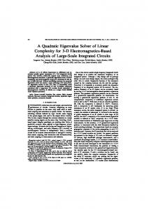
Figure 8 focuses on the solutions obtained from the final generation. A range of solutions that cost 0-75 $/ha provide reduction of 0-18.5% in atrazine loading. The solutions from the multiobjective optimization model unlike single solution obtained from single objective optimization models provide the decision maker choices to optimize the funds available, which is a constraint in some cases. In other cases where the goal is to obtain a solution to meet the specified TMDL goals in a watershed, the solutions should at least produce the specified reduction; therefore the optimized solution that costs the least for achieving the particular water quality goals is selected. However, if equal weight is to be given to the two objectives of pollution reduction and net cost increase, the solution that is closest to the origin is selected, i.e. a solution for which Eq. 8 is the least.
( f ( x )) + ( g ( x )) 2
2
Eq. 8
Figure 9 demonstrates the spatial placement of BMPs in the watershed, at the HRU level. Figure 9 (a) shows the placement of BMPs that achieve the best pollution reduction for a net cost increase of $75/ha in the watershed. The BMP placement corresponding to an intermediate solution is given in Figure 9 (b), where the BMP implementation has a net cost increase of $21.5/ha. Figure 9 (c) represents the base scenario with no increase in cost and no atrazine reduction in the watershed.
15
100 Solutions (Final Generation) Initial Pesticide yield
90 80
Net Cost ($/ha)
70 60 50 40 30 20 10 0 0.58
0.6
0.62
0.64 0.66 0.68 Pesticide Yield (ppb)
0.7
0.72
0.74
Figure 8. Pareto-optimal front after the final generation of the pesticide model
SUMMARY AND CONCLUSIONS Watershed level placement of BMPs to achieve maximum NPS pollutant reduction with minimal increase in BMP implementation costs is an active area of research. This requires finding an optimal solution from many millions of feasible alternatives for the selection and placement of BMPs. The BMP optimization problem requires searching a large variable space to get an optimal solution. Genetic algorithms (GA) are search techniques which search the solution space globally and hence perform better than the local search techniques (for example back propagation, SIMPLEX (Nelder and Mead, 1965) to solve problems with large variable space. Most previous works in developing models for this problem have used GA for optimization by considering the two objectives of cost increase and pollution reduction individually by placing a constraint on one objective while optimizing the other. The drawback with this approach is that some solutions might be lost because the two objectives are considered separately. We have addressed this problem with the development of a multi-objective optimization algorithm framework that considers both these objectives simultaneously. Also the previous models developed were confined to either field scale or small watersheds (area