greatest fuel saving achieved experimentally for a warm engine was 3.6% over a .... is used for gear shift strategy optimisation on the NEDC, and determines the fuel savings which are ..... search was conducted to find the optimal shift strategy.
Vagg, C., Brace, C. J., Wijetunge, R., Akehurst, S. and Ash, L. (2012) Development of a new method to assess fuel saving using gear shift indicators. Proceedings of the Institution of Mechanical Engineers, Part D: Journal of Automobile Engineering, 226 (12). pp. 1630-1639. ISSN 0954-4070 Link to official URL (if available): http://dx.doi.org/10.1177/0954407012447761 Copyright University of Bath 2012. Published by Sage at http://dx.doi.org/10.1177/0954407012447761
Opus: University of Bath Online Publication Store http://opus.bath.ac.uk/ This version is made available in accordance with publisher policies. Please cite only the published version using the reference above. See http://opus.bath.ac.uk/ for usage policies. Please scroll down to view the document.
Development of a New Methodology to Assess Fuel Saving Using Gear Shift Indicators
ABSTRACT European regulations set the emissions requirements for new vehicles at 130 g CO 2/km with an additional 10 g CO2/km to be achieved by additional complementary measures, including gear shift indicators (GSIs). However, there is presently little knowledge of how much fuel or CO 2 could actually be saved by the introduction of GSIs, and there is no consensus on how these savings should be quantified. This study presents a procedure which allows these savings to be quantified over a New European Drive Cycle (NEDC) and explores the trade-off between fuel savings and drivability. A vehicle model was established and calibrated using data obtained from pedal ramp tests conducted at steady speed using a chassis dynamometer, significantly reducing the time required to generate a calibration data set when compared with a steady state mapping approach. This model was used for the optimisation of gear shift points on a NEDC for reduced fuel consumption subject to drivability constraints. During model validation the greatest fuel saving achieved experimentally for a warm engine was 3.6% over a NEDC within the constraints imposed using subjective driver appraisal of vehicle driveability. The same shift strategy for a cold start NEDC showed a fuel saving of 4.3% over the baseline, with corresponding savings in CO 2 of 4.5% or 6.4 g CO2/km. For both hot and cold tests the savings were made entirely in the urban phase of the NEDC; there were no significant differences in fuel consumption in the extra-urban phase. These results suggest that the introduction of GSIs could make a substantial impact, contributing significantly towards the 10 g CO2/km to be achieved by additional complimentary measures when assessed in this way. It is not clear whether these savings would translate into real world driving conditions, however for
legislative purposes an assessment procedure based on the NEDC remains a logical choice for simplicity and continuity.
Keywords: Gear Shift Indicator, Gear shift strategy, Eco-driving, Fuel economy, NEDC, Additional complimentary measures, Transient engine mapping
1. INTRODUCTION 1.1 REGULATORY FRAMEWORK UN/ECE Regulation No 83 [1] describes specific testing procedures for determining fuel consumption and tailpipe emissions of passenger and light commercial vehicles during type approval. The Type 1 test is used to verify tailpipe emissions and fuel consumption during the New European Drive Cycle (NEDC) on a chassis dynamometer after a cold start. For vehicles with manual transmission the drive cycle defines both the speed trace of the vehicle, as well as the points at which the driver must change gear. The NEDC may be regarded as comprising two parts: urban and extra urban, as defined in Annex 4a of UN/ECE Regulation No 83. Part 1 consists of four repetitions of the Elementary Urban Cycle, and Part 2 consists of a single Extra-Urban Cycle, as shown in Figure 1.
Figure 1 – The New European Drive Cycle broken down into Part 1 (Urban) and Part 2 (ExtraUrban). Following concerns that motor vehicle manufacturers would not meet their commitments to reduce new car CO2 emissions to 140 g CO2/km by 2008-9, the European Union issued Regulation (EC) No 443/2009 [2]. This Regulation sets the average emissions requirement for the new car fleet in the European Community in 2012 at 130 g CO2/km, with an additional 10 g CO2/km to be achieved by additional complimentary measures such as gear shift indicators (GSIs)*. Under Regulation (EC) No 661/2009 [3] GSIs are a requirement for all cars type approved from 1 November 2012.
Interestingly, under Annex 14 of UN/ECE Regulation No 83, hybrid electric vehicles (HEVs) fitted with GSIs have been permitted to ignore the standard gear shift points and instead use the speed trace designed for vehicles with automatic transmission with gear shifts effected by the driver as advised by the GSI. For those HEVs equipped with a GSI it is reasonable to speculate that some of the fuel savings made during a Type 1 test result from the exemption from the standard gear shift schedule. *
A gear shift indicator is defined by Regulation (EC) No 661/2009 as “a visible indicator recommending that the driver shift gear”.
There is not yet an agreed method to determine the real fuel or CO 2 savings that will be delivered by GSIs, and therefore whether the intended 10 g CO2/km savings to be delivered partly by GSIs is realistic. The Department for Transport commissioned a report, undertaken by AEA and Millbrook Proving Ground, to assess the potential impact of GSIs and to propose a method to quantify this [4]. This report highlighted the lack of high quality published data on the subject, and also noted that the savings achieved would vary considerably for vehicles of different mass, fuel, usage patterns, etc. One of the proposed methods to quantify the savings achieved by a GSI was to perform Type 1 tests first following the standard legislative gear shift points and then those suggested by the GSI, and to compare the two sets of results. This was undertaken for 3 vehicles, for which results are summarised in Table 1. For each test configuration one test was completed (a total of two tests per vehicle), and the nominal repeatability of the chassis dynamometer with an experienced user and driver (2% Coefficient of Variance (CV)) was deemed sufficient. Table 1 – CO2 savings achieved by following the GSI [4].
BMW Mini VW Golf Ford Transit
Part 1 6.45 0.12 13.53
% Reduction in CO2 Part 2 NEDC Overall 2.15 4.16 -0.23 -0.07 1.65 6.68
Ngo et. al. [5] showed fuel savings of 11.2% in Part 1 of the NEDC when optimising the shift strategy of a Mitsubishi Colt equipped with Automated Manual Transmission. Casavola et. al [6] showed savings of 9.1% over a NEDC when optimising the shift strategy of a small car in a simulation environment.
1.2 OBJECTIVES This study responds to the present state of legislation and the needs identified in the literature to achieve the following objectives: Objective 1: Propose a methodology to determine the optimum gear shift schedule for reduced fuel consumption subject to drivability constraints, to aid future development of GSI logic. Objective 2: Follow the procedure set out by AEA/Millbrook in order to add to the body of high quality published data on the efficacy of GSIs, thereby responding to the need identified.
2. METHODS In order to meet the defined objectives this study presents the development of a simulation tool based on empirical test results and supported by subjective appraisal of vehicle drivability. The resulting simulation is used for gear shift strategy optimisation on the NEDC, and determines the fuel savings which are possible through this alone. The methodology used to optimise the gear shift schedule is explained, which allows the trade-off between reduced fuel consumption and drivability to be explored. Empirical test results for the validation data sets are presented, following the procedure outlined by AEA/Millbrook.
The test vehicle used in this investigation was a Citroen Berlingo, a light commercial vehicle, for which full specifications can be seen in Table 2. Experiments were carried out on the chassis dynamometer test facility at the University of Bath. Two methods of emission measurement were used: tailpipe gas sampling (CO2 tracer method), and bag analysis. In the former, a continuous sample of tailpipe gas is passed through emissions analysers real-time and recorded at 10Hz. In the later, a continuous sample of the same gas is collected in a bag throughout each Part of the test. The contents of each bag are passed through analysers post-test in order to infer the total mass of emissions throughout the test. Bag analysis
is typically more accurate, but does not allow any insight into the instantaneous emissions production [7]. In both cases a carbon balance approach was used to find the fuel consumption. The test facility is temperature controlled, and was maintained at 25°C throughout all tests. Brace, Burke, and Moffa [8] demonstrated that during chassis dynamometer fuel consumption measurement three of the most influential variables are vehicle battery charge, oil level and tyre pressures. Regular vehicle checks were performed in order to limit the effects of these variables. Table 2 – Specifications of the test vehicle. Vehicle Type Vehicle Model Fuel Engine Kerb weight (kg) Transmission – Gear 1 Transmission – Gear 2 Transmission – Gear 3 Transmission – Gear 4 Transmission – Gear 5 Transmission – Final Drive
Citroen Berlingo LX 625 L1 Diesel 1.6HDi 90hp 1354 11/38 (0.290) 15/28 (0.536) 32/37 (0.865) 45/37 (1.216) 50/33 (1.515) 17/73 (0.233)
2.1 VEHICLE MAPPING A backward facing computational model of the vehicle driveline was built using Simulink. In order to determine the fuel consumption characteristics of the vehicle a series of mapping tests were conducted. These tests were performed on the chassis dynamometer rather than by testing the engine separately. The advantage of this approach is that a direct link may be drawn between tractive force at the wheels and fuel consumption, accounting for gearbox and tyre losses in the measurement rather than adding these in later. Ideally tests should then be performed in each gear in order to account for differing efficiencies and losses, and therefore populating steady state maps would be a considerable undertaking. For this reason the driveline was mapped by using the dynamometer in closed-loop speed control mode at a range of speeds, and applying a throttle ramp to achieve the full range of tractive effort. Each throttle ramp was
applied over 2 minutes, held briefly, and then released over a period of 2 minutes. An example of the data collected by this method in fourth gear is presented in Figure 2; some speeds have been omitted for clarity.
Figure 2 – Fuel consumption data obtained in fourth gear using the throttle ramping technique. The advantage of this methodology is that it provides a fuller picture of engine performance than may be obtained through steady state testing. However, whilst the traces are very repeatable at high speeds and loads, at low speeds and loads there is considerable hysteresis, which produces ambiguity. Another observation from this exercise is that the engine does not normally produce positive tractive force until the throttle signal is >25% and the tractive force production is typically saturated at approximately 70% throttle. Consequently although 4 minutes of transient data is collected for each speed, only about 45% of this is useful information. Furthermore, since the NEDC is a relatively low power drive cycle, a large portion of this usable map is never visited. If this exercise were to be repeated the authors would suggest considering these facts, and perhaps modifying the throttle ramp trace to ensure accuracy is maximised in the areas of the engine map which are of most interest.
The fuel consumption data recorded by the tailpipe gas sampling (CO2 tracer) method were parameterised as a set of quadratic surfaces, with one surface per gear. Manipulation of these surfaces allowed plots such as those presented in Figures 3 and 4 to be constructed which are useful when considering possible gear shift strategies. Note that the engine torque has been calculated from the tractive force at the wheels assuming 100 per cent transmission efficiency. For this reason it is referred to as Net Engine Torque and represents the useful torque delivered by the engine to the wheels.
Figure 3 – Brake Specific Fuel Consumption (BSFC) plot and torque limit curve constructed from third gear data. Contours show BSFC is units of g/kWh. Net Engine Torque represents useful engine torque delivered to the wheels, accounting for driveline inefficiencies.
Figure 4 – Constant velocity fuel consumption of the vehicle in each gear, predicted by the quadratic engine model.
2.2 MODEL VALIDATION In order to validate the model a set of heuristic gear shift schedules were designed with reference to Figures 3 and 4, to give a range of shifting behaviour. Each upshift was defined at a road speed, which implies an engine speed as defined by the vehicle transmission ratios. Since the objective of minimising fuel consumption inevitably leads to upshifting as soon as possible a number of constraints were placed on the possible gear shift schedules: each upshift must occur at a higher road speed than the previous, and a minimum post-upshift engine speed was defined in order to ensure drivability.
The speed trace defined in UN/ECE Regulation No 83 for manual vehicles includes steady speed periods of 2 seconds which correspond to gear shift points. Since gear shift points were to be moved throughout this investigation it was decided instead to use the speed trace defined for vehicles with an automatic transmission, which does not include these sections; this is the procedure used for testing HEVs with a special shifting strategy. The gear shift points for the standard (baseline) schedule used here are fixed at
the times defined in UN/ECE Regulation No 83. Since the shape of the speed trace for automatic vehicles is subtly different to that for manual vehicles the upshift speeds quoted with respect to this speed trace differ very slightly to the standard upshift speeds using the manual trace; these differences are not considered significant. Using the standard gear shift schedule (applied to the speed trace for automatic vehicles) the engine speed after an upshift is typically in the region 1300-1700rpm for the vehicle described in Table 2. Three modified schedules were designed such that the minimum engine speed after upshifting was greater than 1300, 1200, and 1100rpm. These schedules shall be referred to as A, B, and C for convenience and the standard schedule shall be referred to as STD. Downshifts were effected when the vehicle speed dropped 0.5kph below each upshift speed to allow hysteresis and avoid excess shift busyness, and the de-clutch points were unaltered from the standard schedule. Table 3 shows the road speed (kph) at which gears 2 to 5 were engaged for each schedule. Table 3 – Upshift speeds (kph) for each gear schedule. Note that the STD shift speeds are found by taking the timestamp of the shift in the manual trace, and applying this to the automatic speed trace.
Gear 2 Gear 3 Gear 4 Gear 5
STD 15.1 32.7 50.1 68.5
Gear Shift Schedule A (1300) B (1200) 21.5 21.5 32.0 30.0 46.9 41.9 65.3 65.3
C (1100) 19.3 30.0 36.9 50.0
It is standard test procedure for the NEDC to be conducted from a cold start, and as such it is preferable to conduct one test per day. However, the simple engine model used here is only able to simulate a warm engine and it was therefore decided to test the above schedules from a hot start, with reference to engine sump oil temperature. Therefore the vehicle was driven at a high speed until the engine oil temperature reached 90°C immediately prior to the test.
The effect of modifying the shift speeds on gear selection is demonstrated in Figure 5, which shows traces of vehicle speed divided by engine speed in the first Elementary Urban Cycle of a NEDC for each gear shift schedule. During the second microtrip† schedule STD only uses gears 1-2 whilst schedules A, B and C all make use of gear 3. Similarly in the third microtrip schedule STD only uses gears 1-3 whilst schedules A and B make use of gear 4, and schedule C also uses gear 5. The spikes which are frequently seen towards the end of a microtrip are a result of the driver de-clutching and a subsequent drop in engine speed. These should not be misinterpreted as a brief upshift.
Subjective driver feedback was collected for each gear shift schedule to assess the drivability of the vehicle. This feedback indicated that schedule C was close to the acceptable limit of drivability; it was possible to achieve the speed trace without the engine nearing the stall condition, but the vehicle was becoming noticeably more difficult to drive due to reduced torque reserve‡. In order to maintain a realistic driving style with a suitable torque reserve it was decided not to further reduce the upshift speeds.
†
A microtrip is defined as beginning when the vehicle is accelerated from rest to have positive velocity, and ends when the vehicle returns to rest. Thus the Elementary Urban Cycle consists of three microtrips and the NEDC consists of 13 microtrips. ‡ Torque reserve is the difference between current engine torque and maximum engine torque at the current engine speed. In test cycle driving it is important to have adequate torque reserve so that if the current vehicle speed falls below the required vehicle speed this can be quickly corrected. In real world driving torque reserve determines how responsive the vehicle feels to a step input in throttle.
Figure 5 – Traces showing the gears engaged during the first Elementary Urban Cycle.
3. RESULTS Cumulative fuel use and emissions figures quoted from this point onwards are measured using the bag analysis method for increased accuracy. Instantaneous fuel consumption measured according to the CO2 tracer method was used only to check the behaviour of the model was sensible.
3.1 HOT START TESTS Test results for the complete NEDC performed from a hot start are presented in Table 4 for each gear shift schedule. As can be seen, moving the gear shift points has a significant impact on fuel consumption, and lowering the minimum engine speed constraint reduces the total fuel use. During the engine mapping work undertaken for model development it was found that the vehicle engine was more efficient when operating at low speed and high load (Figure 3). This finding is typical of diesel engines and so it is not surprising that reducing engine speed causes a reduction in fuel use. Table 4 also shows p-values resulting from two-tailed unpaired t-tests comparing schedules A, B and C with schedule STD, showing that the
fuel savings for schedule A are not significant at the 95% confidence level, whilst those for B and C are significant with confidence levels of 99% and 99.9% respectively. Table 4 – Fuel consumption changes for hot start tests. Number of repeats (n) Fuel Used (g) Standard Deviation (SD) (g) Coefficient of Variance (CV) (%) Fuel saving over STD (%) Statistical significance (p)
STD 6 445.5 4.90 1.10 -
A 4 439.4 4.31 0.98 1.4 0.0767
B 5 435.4 5.23 1.20 2.3 0.0089
C 5 429.6 2.71 0.63 3.6