Development of a Resource Allocation Model ... - Semantic Scholar

sustainability Article

Development of a Resource Allocation Model Using Competitive Advantage Sangwon Lee 1 , Suneung Ahn 2 , Changsoon Park 3 and You-Jin Park 4, * 1 2 3 4

*

Department of Interaction Science, Sungkyunkwan University, Seoul 03063, Korea; [email protected] Department of Industrial and Management Engineering, Hanyang University, Ansan 15588, Korea; [email protected] Department of Mechanical Engineering, Hanyang University, Ansan 15588, Korea; [email protected] School of Business Administration, Chung-Ang University, Seoul 06974, Korea Correspondence: [email protected]; Tel.: +82-02-820-5744

Academic Editor: Sangkyun Kim Received: 30 September 2015; Accepted: 27 January 2016; Published: 29 February 2016

Abstract: In general, during decision making or negotiations, the investor and the investee may often have different opinions which result in conflicts. So, an objective standard to mitigate potential conflicts between investors and investees should be provided since it is highly important that rational decisions must be made when choosing investments from various options. However, the models currently used come with some problems for several reasons, for instance, the arbitrariness of the evaluator, the difficulty in understanding the relationships that exist among the various investment options (that is, alternatives to investments), inconsistency in priorities, and simply providing selection criteria without detailing the proportion of investment in each option or evaluating only a single investment option at a time without considering all options. Thus, in this research, we present a project selection model which can enable reasonable resource allocation or determination of return rates by considering the core competencies for various investment options. Here, core competency is based on both performance and ability to create a competitive advantage. For this, we deduce issue-specific structural power indicators and analyze quantitatively the resource allocation results based on negotiation power. Through this, it is possible to examine whether the proposed project selection model considers core competencies or not by comparing several project selection models currently used. Furthermore, the proposed model can be used on its own, or in combination with other methods. Consequently, the presented model can be used as a quantitative criterion for determining behavioral tactics, and also can be used to mitigate potential conflicts between the investor and the investee who are considering idiosyncratic investments, determined by an interplay between power and core competency. Keywords: resource allocation; competitive advantages; idiosyncratic investments; power

1. Introduction Conflicts often arise when there is a certain gap between purposes or expected outcomes of investors (e.g., decision makers, government, etc.) and investees (e.g., proposers, developers, etc.) due to many reasons, for example, a lack of both structural analysis or objective logic of investment. Generally, the investment decision is made through the evaluation of several options bringing both return and risk. Therefore, investors use various methods when allocating resources, which can involve descriptive assessment; the score method, the Delphi method agreed upon by experts [1], the pair-wise method through comparisons between alternatives [2,3], the utility theory based on the preferences of investors [4], risk analysis [5,6], regression and correlation analysis [7,8], multi-task analysis [9], etc.

Sustainability 2016, 8, 217; doi:10.3390/su8030217

www.mdpi.com/journal/sustainability

Sustainability 2016, 8, 217

2 of 13

Resource allocation models currently used come with some problems stemming from, for instance, the arbitrariness of the evaluator, the difficulty in understanding the relationships among various options, and inconsistency of priorities. Therefore, to resolve these problems, diverse combined methods have been proposed, for example, AHP (Analytic Hierarchy Process) and Integer Programming [10], AHP and linear programming [11], AHP and fuzzy [12], ANP (Analytic Network Process) and fuzzy [13], and multi-criterial analysis considering revenue [14]. However, since the existing models also pose problems in simply providing simple selection criteria without detailing the proportion of investment in each option or evaluating only one single investment option at a time without considering all the options, it is consequently very difficult to properly allocate resources to the options. An investment decision, in general, is made as a result of negotiation between investors and investees. Their relationship is dependent on the motivation of each party, and it is inevitable that conflicts arise. So, in this case, exerting particular powers which lead to the assignment of specific tasks to both investors and investees may be a way to manage the conflicts. Here, the power is defined by the dependency on investment decision-making [15–17]. Therefore, sometimes, investors and investees may be required to make idiosyncratic investments based on the perceived strength of each other [18,19]. An investment follows on from a negotiation between the investor and investee, which involves an interplay of power leading to the ultimate decision to invest in a particular option. Negotiation power is not only drawn from special qualifications or relationships between the investor and investee but also from the ability to influence each other [20]. The negotiation power stems from issue-specific structural power and behavioral power [21]. Structural power represents a negotiator’s relative position, which is also determined by a number of physical elements (e.g., capital, information, technology, strategy, quality, etc.) while behavioral power is related to negotiation behavior, and is presented through negotiation tactics. Particularly, structural power is related to core competency which involves both performance and ability to create a competitive advantage; for example, technology, market share, brand power, capital strength, etc. [22,23]. The core competencies can be identified through comparison of competitors. Since an investor demands an investee to achieve their best in order to build competitive advantage, the investor has to make difficult investment decisions based on the perceived core competencies of the investee. When the investor and the investee have different aims or expected outcomes to investments during their negotiations, it results in conflicts. Therefore, it is necessary to present an objective standard to mitigate conflicts between the investor and the investee, one that can be continually improved upon with the ultimate goal of making rational investment decisions. Above all, clear, fair, and consistent criteria are needed for reviewing various investment options in order to conduct an effective negotiation. Reservation value is one of the criteria, and there is no difference between completion and breakdown of negotiation [24]—this can be obtained through BATNA (best alternative to a negotiated agreement) [25]. The results show that a BATNA can be a criterion for finding the balance point between investors and investees for problems in allocating investments. This paper presents a project (which is regarded as an investment option) selection model which can enable the most appropriate resource allocation based on the core competencies of investees. The presented model can mitigate conflicts in investment decision-making between the investor and the investee when considering idiosyncratic investments. Moreover, the model can be used in finding the best options in the process of negotiation. In Sections 2 and 3 we present preliminaries, a resource allocation model, and a decision-making process in terms of competitive advantages. In Section 4, we show examples of the model. Section 5 concludes.


3 of 13

2. Preliminaries This study begins with an assumption that an investor invests in various options and has a MARR (minimum attractive rate of return). An investment is made based on the evaluation of investment options, and the evaluation is related to the competitive advantages of the various investment options. Therefore, the investor should determine the core competencies of these options in order to ultimately determine the allocation of investable resource and the rate of return [26]. This study also assumes that the evaluation measures are mutually exclusive and may be comparable. The investor may decide the scale of investment and return methods based on the values of the measures. The scale of investment can be divided according to the values of assessment items as the measures are mutually exclusive and comparable. For example, we consider two investment options—that is, A and B—and set technology and business as measures of evaluation. The evaluation results of options are shown in Table 1. The sum of the evaluation values for technology and for business are 0.9 and 1.1, respectively, if the investor has to invest 1 in each option A and B. Table 1. The evaluation of investment options.

Evaluation Fields Fields

Technology Business Sum

Investment Options A B 0.5 0.4 0.5 0.6 1 1

Sum 0.9 1.1 2

The competencies and competitive advantages of investment options can be identified by their evaluation values. An investor requires a safe investment and high returns while the investee attempts to guarantee a certain amount of investment and as little return rate as possible for the investor. Therefore, the investee receives an idiosyncratic investment above other ordinary investees, and also an investor simultaneously lowers their own risk by investing its resources based on core competencies. The core competency determines the structural power of investors. However, the values of evaluation and the scales of investment are not linearly proportional. If the linearly proportional allocation is reasonably based on the values, the usual problems associated with an idiosyncratic investment should not arise. In the example above, if the technology of the two investment options is common, the investor should invest more in option B than in A because of the factor “business”. Thus, in this study, the process is modeled in terms of core competencies. 3. Model 3.1. Development of a Resource Allocation Model The total investment (Ii ) in a certain investee i (i = 1, 2, . . . ) can be composed according to the rating values (Pij ) of assessment items j (j = 1, 2, . . . ), and so the classified scale of investment (Iij ) can be calculated from Equation (1). Pij Iij “ ř ˆ Ii j Pij

(1)

Investees or investment options acquiring a high rating value for a particular assessment item can be determined, which means that the investee (or investment option) has a higher competency in this field than others because the evaluation value of an investee indicates competency and also corresponds to structural power. In this case, it is necessary to normalize the rating values using a criterion such as the sum of the value or weight. So, the proportion of rating value (Pij ) and the sum of ř rating values ( Pij ) in the same assessment item (j) can be the structural power, and this structural power indicator (λij ) represents the relative position of power in the same assessment item.


4 of 13

Pij λij “ ř i Pij

(2)

If the structural power indicator (λij ) of an investee is relatively high, the investee has a core competency for an assessment item and can induce favorable investment from an investor. Therefore, we need to obtain the virtual scale of investment considering a core competency, that is, the relative investment of rating value (RIij ). The relative investment of rating value (RIij ) is proportional to the multiplication of the investment regarding only evaluation values (Iij ) and the structural power indicator (λij ) as shown in the following Equation (3). RIij 9λij ˆ Iij

(3)

Since the relative investment of the rating value (RIij ) is a proportional model using the structural power indicator (λij ), it is difficult to compare the relative investment of the rating value (RIij ) and the classified scale of investment (Iij ) directly. So, we should value both investments (RIij and Iij ) as equal for a certain common assessment item (j) as shown in Equation (4). ÿ

RIij “

i

ÿ

Iij

(4)

i

Therefore, the relative investment of rating value (RIij ) can be obtained from Equation (5) using Equations (1)–(4), and the relative investment of a certain investee (i) is the sum of the relative investment of rating value (RIij ) as shown in Equation (6). If the RIij of a certain investee (i) is greater than the Iij , the investee (i) is not recognized to have a competitive advantage. For this reason, conflict arises or an idiosyncratic investment can be induced by the investee. ř ř i Iij i Iij RIij “ λij ˆ Iij ˆ ř “ Pij ˆ Iij ˆ ř (5) i λij Iij i Pij Iij ÿ RIi “ RIij (6) j

Since the relative return, considering rating value (RUij ), is proportional to multiplication of RIij and Uij , the relative return considering rating value (RUij ) can be obtained from multiplying the relative investment of rating value (RIij ) by the relative rate of return considering rating value (Rαi ) as shown in Equation (7). The return (Uij ) can be easily obtained from the multiplication of the classified scale of investment (Iij ) and the rate of return (αi ). Here, the rate of return (αi ) means the return of the real investment (Iij ) and the efficiency. Thus, the relative rate of return (Rαi ) is a core competency which reflects the actual rate of return (αi “ Uij {Iij ). However, it is difficult to induce Rαi directly. RUij 9 RIij ˆ Uij

(7)

As already mentioned, the relative return considering rating value (RUij ) is a proportional model involving the core competency. However, since it is difficult to compare RUij and the Uij , we should make the sum of both returns (RUij , Uij ) equal for a certain common assessment item (j) as shown in Equation (8), and the relative return considering rating value (RUij ) can be obtained from Equation (9) using Equations (7) and (8). Consequently, the relative return considering rating value (RUi ) for an investee (i) can be represented by the sum of RUij as shown in Equation (10). ÿ i

RUij “

ÿ

Uij

(8)

i

ř i Uij RUij “ RIij ˆ Uij ˆ ř i RIij Uij

(9)


5 of 13

RUi “

ÿ

RUij

(10)

j

If the relative return considering rating value (RUij ) of a certain investee (i) is greater than the Uij , the investee (i) has a competitive advantage, and thus the investee (i) is more likely to make a good return and carry a low risk. The return of investment (Ui ) can be obtained from the multiplication of the actual investment (Ii ) and the rate of return (αi ) as shown in Equation (11), and also RUi can be obtained from the multiplication of RIi and Rαi . If we would take advantage of RIi , RUi should be represented as the multiplication of Rαi and Ii as shown in Equation (12) because it is difficult to compare Rαi to αi directly. Here, we note that the investment (Ii ) in investee (i) and the relative investment (RIi ) are the same, and the return (Uij ) of an investee (i) and the relative return (RUij ) are the same as well. Therefore, the sum of the rate of return αi for the investee is the same as the total of Rαi as shown in Equation (13). Ui “ αi ˆ Ii

(11)

RUi “ Rαi ˆ Ii ÿ ÿ αi “ Rαi

(12)

i

(13)

i

As described above, the rate of return (αi ) means the return of the real investment (Iij ) and the efficiency. Similarly, the relative rate of return (Rαi ) means the relative return of the real investment (Iij ) and the efficiency considering the competitive advantage. If the rate of return (αi ) is greater than the relative rate of return considering the rating value (Rαi ), this means that the actual investment (Ii ) is more than the investment. If αi is smaller than Rαi , this means that the actual investment (Ii ) is less than the investment. Therefore, it is necessary to reallocate the portion of over-investment in the investee to the under-invested investees. Additionally, when considering the same scale investment for each investee, over-investment or under-investment may be prevented by adjusting the rate of return (αi ). 3.2. Resource Allocation If the relative return of investee (RUi ) is greater than the return (Ui ) when core competencies are considered, it means that the efficiency of investment return is high and also the structural power of negotiation is strong, but the investee may receive a relatively poor investment. On the contrary, if RUi is smaller than Ui when core competencies are considered, it means the efficiency of investment return is low and the structural power of negotiation is weak, but the investee may receive a better investment. Therefore, it is important that the investor recognizes the merit of the investee, and this reduces the investment risk. As mentioned above, Rαi means the efficiency of the relative return (RUi ), since the relative rate of return (Rαi ) represents the return rate per one unit of investment. However, if the deviation of the relative rate of return (Rαi ) and the average of the relative rate of return (Rα) seems quite large, then ˘2 ř` it can be regarded as a wrong investment because the greater the deviation ( Rαi ´ Rα ) is, the i

greater the chance that conflict may arise during negotiation. However, since it is difficult to derive the Rα directly, we should take advantage of Rαi and the average of return (α) because Rα “ α. Therefore, the investor attempts to mitigate conflict during the negotiation and the risk from the return ř by minimizing the deviation ( pRαi ´ αq2 ). i

The relative return (RUi ) can be obtained from the multiplication of the scale of investment (Ii ) and the relative rate of return (Rαi ). RUi is the efficiency of core competency in accordance with the Ii , and also can be interpreted as the relative possibility of the investment return (Ui ). Therefore, it is best that an adjusted resource allocation (Ii ) maintains the efficiency (RUi ) of a core competency on the fixed return rate (for example, Rαi “ Rα “ α). The best resource allocation (Ii˚ ) can be the


6 of 13

multiplication of RUi and α. Also, Ii˚ is obtained using the formula development and the componendo and dividendo rule as shown in Equations (14) and (15). The average of the relative rate of return (Rα) ř ř is composed of the total investment ( Ii ) and the total relative return ( RUi ). We can find Rα “ α i

i

using Equations (8), (13), (14) and (15). In this case, α is the acceptable rate of return and the policy of the investor. In addition, it is the best option of the return rate (α˚i ) and an adjusted return rate maintains the efficiency (RUi ) of a core competency in the fixed investment (constant Ii ), as shown in Equation (16). ř ř RUi U RU1 RUi RU2 i “ ¨¨¨ “ ˚ “ ¨¨¨ “ ř “ ři i “ α (14) “ I I1˚ I2˚ Ii i i i Ii Sustainability 2016, 8, 217

6 of 13

ÿ RUi RU Ii “ Ii˚ “ ř i ˆ RU α i i ∗ i

∑

α˚i “ ∗

RUi constant Ii

(15) (15)

(16) (16)

4. Examples 4. Examples We reviewed the derivation process of the best option for an investment negotiation using

a simpleWe example and the sensitivity of resource allocation to core competency. reviewed the checked derivation process of the best option for an investment negotiation using a Finally, we simple example and checked the sensitivity of resource allocation to core competency. Finally, we also compared the proposed model to the project selection models. also compared the proposed model to the project selection models.

4.1. The Derivation Process of the Best Option 4.1. The Derivation Process of the Best Option

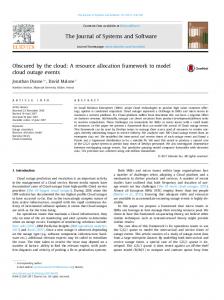
The best resource allocation option can be derived using the proposed model as per the example ř of TableThe best resource allocation option can be derived using the proposed model as per the example 1 (see Figure 1). Both the total investment ( i Ii ) and the rate of return (αi ) are assumed to be a of Table 1 (see Figure 1). Both the total investment (∑ ) and the rate of return ( ) are assumed to be value of 1 for convenience. Because the values of assessment items are 0.9 for technology and 1.1 for a value of 1 for convenience. Because the values of assessment items are 0.9 for technology and 1.1 business, according to this evaluation, business has more competitive advantage than technology. Even for business, according to this evaluation, business has more competitive advantage than technology. though the rating values of option A (technology and business) are the same (PA,Tech. = = PA,Busi. = 0.5), Even though the rating values of option A (technology and business) are the same ( , . , . = the 0.5), the implicit meaning of the values can be different. implicit meaning of the values can be different.

Figure 1. Derivation process of the best option. Figure 1. Derivation process of the best option.

The issue‐specific structural power of the option A for the technology is identified in the overall The issue-specific structural power of the optionpower A for indicator the technology is identified in the overall power of the options’ technology. So, the structural of the option A technology power, of . the options’ technology. So,the thesame structural power indicator of the optionof A the technology is 0.5/0.9 (0.5556 > 0.5). In way, the structural power indicator option A λ A,Tech. business 0.5/11 is , . and A , business . because they use different references ( •, 0.9, •, 1.1). . . The investment of option A for technology ( , . ) is 0.25 (0.5/2). However, the relative investment ( , 0.25) because the investment of technology (∑ , . ) is 0.2744 (> , . . ) is 0.45 considering the core competency. In addition, the , 0.25 and 0.2254, and the . , . return of option A technology , . is 0.25. However, the relative return of option A for the technology 0.25) as it refers to the core competency. Therefore, the , . is 0.2976 (> , . option A has a competitive advantage in the field of technology ( 0.2976 , 0.25). , . .


7 of 13

λ A,Busi. is 0.5/11 (0.4545 < 0.5). However, it is not right to add up the λ A,Tech. and λ A,Busi. because they use different references (λ ,Tech. “ 0.9, λ ,Busi. “ 1.1). The investment of option A for technology (I A,Tech. ) is 0.25 (0.5/2). However, the relative investment (RI A,Tech. ) is 0.2744 (> I A,Tech. “ 0.25) because the investment of technology ř ( i Ii,Tech. ) is 0.45 considering the core competency. In addition, the I A,Busi. “ 0.25 and RI A,Busi. “ 0.2254, and the return of option A technology U A,Tech. is 0.25. However, the relative return of option A for the technology RU A,Tech. is 0.2976 (> U A,Tech. “ 0.25) as it refers to the core competency. Therefore, the option A has a competitive advantage in the field of technology (RU A,Tech. “ 0.2976 ą U A,Tech. “ 0.25). On the other hand, option B has a competitive advantage in the field of business (RUB,Busi. “ 0.3484 ą UB,Busi. “ 0.3). Business has a greater competitive advantage than technology does. However, if the actual investment is made according to the rating value, option B has a greater core competency (RUB “ 0.5008 ą RU A “ 0.4992) and, thus, conflict could arise during the investment negotiation. Therefore, the investor reduces investment in option A and increases investment in option B (or increases option A return rate and decreases option B return rate) for the mitigation of risk ˚ “ 49.92% and I ˚ “ 50.08%. Even if the total from return. The best resource allocation option is I A B ř investment ( i Ii ) and the acceptable rate of return (α) are changed, the ratio of the best option does not change. 4.2. The Sensitivity of the Rating Value Variations The proposed model clearly shows that the best option demonstrates core competencies and presents favorable investment conditions. Moreover, even when the values of an assessment item are different among the investment options, the sum of the values could be the same. Therefore, checking the sensitivity of different resource allocation options in this situation (the case that the values are different, but the sums of the values are the same) is necessary. For checking the sensitivity of the options in this case, we consider two situations as examples. The first one is a situation where the values are crossing and changing (see Table 2), and the second one is a situation where the values are sequentially increasing with the average of the other option. Assessment items of the investment ř options are set to 20. Both the total investment ( i Ii ) and the rate of return (αi ) are assumed as 1 for convenience. Table 2. Pattern of return on the crossed values. Assessment Item (j) 1 2 3 4 5 6 7 8 9 10 11 12 13 14 15 16 17 18 19 20 Sum

Rating Value (Pij ) Opt. A Opt. B Sum 0.0025 0.0975 0.1 0.0075 0.0925 0.1 0.0125 0.0875 0.1 0.0175 0.0825 0.1 0.0225 0.0775 0.1 0.0275 0.0725 0.1 0.0325 0.0675 0.1 0.0375 0.0625 0.1 0.0425 0.0575 0.1 0.0475 0.0525 0.1 0.0525 0.0475 0.1 0.0575 0.0425 0.1 0.0625 0.0375 0.1 0.0675 0.0325 0.1 0.0725 0.0275 0.1 0.0775 0.0225 0.1 0.0825 0.0175 0.1 0.0875 0.0125 0.1 0.0925 0.0075 0.1 0.0975 0.0025 0.1 1 1 2

Return (Uij ) Opt. A Opt. B 0.0013 0.04875 0.0038 0.04625 0.0063 0.04375 0.0088 0.04125 0.0113 0.03875 0.0138 0.03625 0.0163 0.03375 0.0188 0.03125 0.0213 0.02875 0.0238 0.02625 0.0263 0.02375 0.0288 0.02125 0.0313 0.01875 0.0338 0.01625 0.0363 0.01375 0.0388 0.01125 0.0413 0.00875 0.0438 0.00625 0.0463 0.00375 0.0488 0.00125 0.5 0.5

Relative Return (RUij ) Opt. A Opt. B 8.429E-07 0.0500 2.664E-05 0.0500 0.0001453 0.0499 0.0004727 0.0495 0.0011943 0.0488 0.0025875 0.0474 0.0050206 0.0450 0.0088816 0.0411 0.0143823 0.0356 0.0212748 0.0287 0.0287252 0.0213 0.0356177 0.0144 0.0411184 0.0089 0.0449794 0.0050 0.0474125 0.0026 0.0488057 0.0012 0.0495273 0.0005 0.0498547 0.0001 0.0499734 3E-05 0.0499992 8E-07 0.5 0.5

Sum of Return 0.05 0.05 0.05 0.05 0.05 0.05 0.05 0.05 0.05 0.05 0.05 0.05 0.05 0.05 0.05 0.05 0.05 0.05 0.05 0.05 1


8 of 13

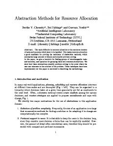
4.2.1. The Case of Crossing Values When we check the changing pattern of the return (Uij ) and the relative return (RUij ) in the case of crossed values (see Table 2), we find the returns of options A and B are the same (U A “ UB ), ř ř ř because i Ii = 1, αi “ 1 and the sum of the option rating values is the same ( j PAj = j PBj “ 1). Nevertheless, the relative returns of options A and B are the same (RU A “ RUB ) because the values of the sum of the same assessment item are constant (PAj ` PBj “ 0.1q. In addition, the sum of the Sustainability 2016, 8, 217 8 of 13 same assessment item return and relative return is also constant (U Aj ` UBj “ RU Aj ` RU Bj “ 0.05). Theitem return and relative return is also constant ( return (Uij ) has also a linear function since the rating value (Pij ) 0.05). has a linear function, and Uij and Pij are linearly proportional. However, this does not explain the idiosyncratic investment decision The return ( ) has also a linear function since the rating value ( has a linear function, and are linearly proportional. However, this does not explain the idiosyncratic investment (see Figure and 2 above). As shown in Figure 2, the relative returns (RU Aj ) for both option A and B are not ) for both option A and a linear decision (see Figure 2 above). As shown in Figure 2, the relative returns ( function form. Precisely, RU Aj is positively shifting from U Aj if it has a competitive advantage B are not a linear function form. Precisely, is positively shifting from if it has a competitive whereas RU Aj is negatively shifting from U Aj if it has a competitive disadvantage. Also, as the advantage whereas is negatively shifting from if it has a competitive disadvantage. Also, competency moves towards extreme positive return or extreme negative return, then RU Aj approaches as the competency moves towards extreme positive return or extreme negative return, then the threshold value. Furthermore, RU A and RUB are the same because positives and negatives are approaches the threshold value. Furthermore, and are the same because positives and offset, although the investment is still in conflict. negatives are offset, although the investment is still in conflict. 0.05

The return

The return of Opt. A The return of Opt. B The relative return of Opt. A The relative return of Opt. B The maximum of the return

0 1 2 3 4 5 6 7 8 9 10 11 12 13 14 15 16 17 18 19 20

(-)

Assessment item

(+)

The structural power of Opt. A

Figure 2. Relative return on the crossed values.

Figure 2. Relative return on the crossed values. 4.2.2. The Case of Increasing Values

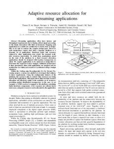
4.2.2. The Case of Increasing Values We examine the changing pattern of the return ( ) and the relative return ( ) in the case of Weincreased values with the average of investment options (see Table 3). We set the rating value and examine the changing pattern of the return (Uij ) and the relative return (RUij ) in the case of the return of the average of options to be constant ( 0.05, 0.025). The return of . . increased values with the average of investment options (see Table 3). We set the rating value and the option A and the return of the other option’s averages are the same ( = 1, . ), because ∑ return of the1, and the sum of option rating values is the same (∑ average of options to be constant (PAver.j “ 0.05,= ∑U Aver.j “1). 0.025). The return of option ř . A and the return of the other option’s averages are the same (U A “ U Aver. ), because i Ii = 1, αi “ 1, We can see the relative return ( ) is not linear because of positive and negative shifting, (see ř ř and theFigure sum of3) option rating valuesof is returns the same ( j PAjlinearly. = j PAs 1). while the maximum increases the “ competency moves toward Aver.j and negative Weextremely positive or negative values, can see the relative return (RU Aj ) is approaches the threshold value. not linear because of positive and shifting, . are not the same because the offset of positives and negatives is incompleteness. (see Figure 3) while the maximum of returns increases linearly. As the competency moves toward If the assessment item is relatively important, the influence of the item is greater and there is extremely positive or negative values, RU Aj approaches the threshold value. RU A and RU Aver. are not more competitive advantage. On the other hand, the competitive advantage is less in the relatively the same because the offset of positives and negatives is incompleteness. ∗ ∗ less important item, so the best option for resource allocation is 54.6% and 45.4%. The . results of the numerical example show that the relationship between the core competency and the structural power points to idiosyncratic investment. Even when the values and the sum of values are different, it shows the same pattern as in Figure 3. Thus, the relevant numerical examples are omitted.


9 of 13


9 of 13

Table 3. Pattern of return on the increasing values.

Rating Value ( ) Return ( ) Relative Return ( ) Assessment Table 3. Pattern increasing Opt. A values. Opt. Aver. Item (j) Opt. A Opt. Aver. Sum of return Opt. Aon the Opt. Aver. 1 0.0025 0.05 0.0525 0.0013 0.025 3.281E‐06 0.0262 Rating Value (P0.0575 Return (U0.025 Relative Return 0.0287 (RUij ) 2 0.0075 0.05 0.0038 9.67E‐05 ij ) ij ) Assessment Item (j) Opt. A Opt. Sum Opt. A Opt.0.025 Aver. Opt. A Opt.0.0308 Aver. 3 0.0125 0.05 Aver. 0.0625 0.0063 0.0004808 1 0.0025 0.05 0.0525 0.0013 0.025 3.281E-06 0.0262 4 0.0175 0.05 0.0675 0.0088 0.025 0.0013875 0.0324 2 0.0075 0.05 0.0575 0.0038 0.025 9.67E-05 0.0287 0.0225 0.05 0.0725 0.025 0.0030274 0.0308 0.0332 3 5 0.0125 0.05 0.0625 0.0113 0.0063 0.025 0.0004808 4 6 0.0175 0.05 0.0675 0.0138 0.0088 0.025 0.0013875 0.0275 0.05 0.0775 0.025 0.0055274 0.0324 0.0332 5 7 0.0225 0.05 0.0725 0.0163 0.0113 0.025 0.0030274 0.0325 0.05 0.0825 0.025 0.0088875 0.0332 0.0324 0.0775 0.0138 0.025 0.0055274 0.0332 6 0.0275 0.05 8 0.0375 0.05 0.0875 0.0188 0.025 0.0129808 0.0308 7 0.0325 0.05 0.0825 0.0163 0.025 0.0088875 0.0324 9 0.0425 0.05 0.0925 0.0213 0.025 0.0175967 0.0287 8 0.0375 0.05 0.0875 0.0188 0.025 0.0129808 0.0308 910 0.0425 0.05 0.0925 0.0238 0.0213 0.025 0.0175967 0.0475 0.05 0.0975 0.025 0.0225033 0.0287 0.0262 0.0975 0.0263 0.0238 0.025 0.0225033 1011 0.0475 0.05 0.0525 0.05 0.1025 0.025 0.0274970 0.0262 0.0238 11 0.0525 0.05 0.1025 0.0263 0.025 0.0274970 0.0238 12 0.0575 0.05 0.1075 0.0288 0.025 0.0324280 0.0213 12 0.0575 0.05 0.1075 0.0288 0.025 0.0324280 0.0213 0.0625 0.05 0.1125 0.025 0.0372024 0.0190 0.0190 1313 0.0625 0.05 0.1125 0.0313 0.0313 0.025 0.0372024 0.1175 0.0338 0.0338 0.025 0.0417721 1414 0.0675 0.05 0.0675 0.05 0.1175 0.025 0.0417721 0.0170 0.0170 1515 0.0725 0.05 0.1225 0.0363 0.0363 0.025 0.0461214 0.0725 0.05 0.1225 0.025 0.0461214 0.0151 0.0151 16 0.0775 0.05 0.1275 0.0388 0.025 0.0502547 0.0135 16 0.0775 0.05 0.1275 0.0388 0.025 0.0502547 0.0135 17 0.0825 0.05 0.1325 0.0413 0.025 0.0541873 0.0121 17 0.0825 0.05 0.1325 0.0413 0.025 0.0541873 0.0121 0.1375 0.0438 0.025 0.0579392 0.0108 18 0.0875 0.05 0.0875 0.05 0.1375 0.025 0.0579392 0.0097 0.0108 1918 0.0925 0.05 0.1425 0.0438 0.0463 0.025 0.0615318 2019 0.0975 0.05 0.1475 0.0463 0.0488 0.025 0.0649858 0.0925 0.05 0.1425 0.025 0.0615318 0.0088 0.0097 Sum 1 1 2 0.5 0.5 0.5464111 0.4536 20 0.0975 0.05 0.1475 0.0488 0.025 0.0649858 0.0088 0.5464111 0.4536 Sum 1 1 2 0.5 0.5

Sum of Return 0.02625 0.02875 Sum of Return 0.03125 0.02625 0.03375 0.02875 0.03625 0.03125 0.03375 0.03875 0.03625 0.04125 0.03875 0.04375 0.04125 0.04625 0.04375 0.04625 0.04875 0.04875 0.05125 0.05125 0.05375 0.05375 0.05625 0.05625 0.05875 0.05875 0.06125 0.06125 0.06375 0.06375 0.06625 0.06625 0.06875 0.06875 0.07125 0.07375 0.07125 1 0.07375 1

0.075

0.05

The return

The return of Opt. A The return of Opt. average The relative return of Opt. A The relative return of Opt. B

0.025

The maximum of the return

0 1 2 3 4 5 6 7 8 9 1011121314151617181920 Assessment item

(-)

(+)

The structural power of Opt. A

Figure 3. Relative return on the increasing values. Figure 3. Relative return on the increasing values.

4.3. Comparison of Proposed Method and Other Models

If the assessment item is relatively important, the influence of the item is greater and there is As mentioned earlier, there are many resource allocation methods such as the descriptive more competitive advantage. On the other hand, the competitive advantage is less in the relatively assessment, score method, the Delphi method, pair‐wise method, utility theory, risk analysis, etc. ˚ “ 54.6% and I ˚ less important item, so the best option for resource allocation is I A Aver. “ 45.4%. The results of the numerical example show that the relationship between the core competency and the structural power points to idiosyncratic investment. Even when the values and the sum of values are different, it shows the same pattern as in Figure 3. Thus, the relevant numerical examples are omitted.


10 of 13

4.3. Comparison of Proposed Method and Other Models As mentioned earlier, there are many resource allocation methods such as the descriptive assessment, score method, the Delphi method, pair-wise method, utility theory, risk analysis, etc. Many different types of composite models have been recently proposed in order to compensate for disadvantages. When a direct evaluation is difficult to make, the investment options can be measured by the score method, and weighted by pairwise comparison (AHP, ANP). After that, resources are assigned to the options by multi-criteria. The proposed model can be used in combination with other methods, or it can be used on its own. Notably, the proposed model can be applied when processing the measured data such as the score method, AHP and ANP. Therefore, we should check whether the proposed model considers the core competencies through comparison with the previous studies of project selection. There are six investment options (P1–P6), and 19 assessment items for the options (see Table 4). The weights of assessment items are derived by ANP [27]. Table 4. Project Selection from Analytic Network Process (ANP). Assessment Item (j)

P1

P2

P3

P4

P5

P6

Sum

1 2 3 4 5 6 7 8 9 10 11 12 13 14 15 16 17 18 19

0.0058 0.0085 0.0069 0.0093 0.0070 0.0126 0.0126 0.0082 0.0191 0.0121 0.0150 0.0056 0.0136 0.0117 0.0107 0.0105 0.0102 0.0105 0.0102

0.0093 0.0136 0.0082 0.0058 0.0046 0.0047 0.0032 0.0041 0.0072 0.0052 0.0169 0.0098 0.0045 0.0050 0.0027 0.0079 0.0119 0.0052 0.0085

0.0070 0.0085 0.0096 0.0081 0.0070 0.0111 0.0111 0.0055 0.0167 0.0121 0.0113 0.0084 0.0113 0.0100 0.0094 0.0092 0.0068 0.0105 0.0102

0.0081 0.0102 0.0041 0.0058 0.0046 0.0047 0.0032 0.0096 0.0048 0.0035 0.0038 0.0126 0.0045 0.0050 0.0027 0.0079 0.0068 0.0039 0.0068

0.0070 0.0085 0.0055 0.0058 0.0058 0.0126 0.0063 0.0055 0.0119 0.0086 0.0113 0.0084 0.0113 0.0100 0.0094 0.0105 0.0102 0.0105 0.0102

0.0058 0.0085 0.0069 0.0093 0.0070 0.0126 0.0126 0.0055 0.0191 0.0138 0.0150 0.0028 0.0136 0.0117 0.0107 0.0105 0.0102 0.0105 0.0102

0.0430 0.0577 0.0411 0.0442 0.0360 0.0584 0.0490 0.0384 0.0787 0.0553 0.0732 0.0476 0.0589 0.0534 0.0456 0.0564 0.0560 0.0511 0.0560

Sum

0.2000

0.1383

0.1836

0.1126

0.1693

0.1962

1

Rank

1

5

3

6

4

2

Sum

0.1972

0.1398

0.1832

0.1180

0.1692

0.1925

Rank

1

5

3

6

4

2

ANP

The score method

1

There is no variation between the ranks when comparing the score method and ANP. However, Rank 1 of the ANP positively shifts from 0.1972 to 0.2, and Rank 2 of the ANP also positively shifts from 0.1925 to 0.1962, while Ranks 5 and 6 of the ANP negatively shift. This is the result of the weighting of assessment items derived by ANP, but it is not considered as the core competencies of competitive advantage. However, since the selection of a project depends on the determined rate of return, a relative investment (Equation (5)) should be made. The results of the proposed model when the total investment ř ( i Ii ) is assumed as 1 are shown in Table 5. We can see there is no variation between the ranks in the comparison of the score method, ANP and the proposed model although, Rank 1 of the proposed model is more positively shifting from 0.2000 to 0.2213 rather than the ANP. Also, Rank 2 of the proposed model is more positively shifting from 0.1962 to 0.2175, but Ranks 5 and 6 of the proposed model are less negatively shifting compared to the ANP (see Figure 4). Although the ANP removes the association of assessment items, and applies the weights of assessment items, the proposed model applies the competitive advantage of the options in the same assessment item.


11 of 13

competitive advantages. Therefore, they are more positively shifting compared to the ANP. However, assessment items 8 and 12 are the same as P3, which means they are less positively shifting. The other assessment items lack competitive advantages. Therefore, the negative shifting has a more serious Sustainability 2016, 8, 217 11 of 13 impact on the result. Table 5. Project Selection from the Proposed Model.

Table 5. Project Selection from the Proposed Model. Assessment Item (j) P1 P2 1 Assessment Item (j) 0.0046 P1 0.0117 P2 2 1 0.0072 0.00460.0185 0.0117 3 2 0.0064 0.00720.0093 0.0185 4 3 0.0112 0.00640.0044 0.0093 0.01120.0035 0.0044 5 4 0.0079 0.00790.0020 0.0035 6 5 0.0144 6 0.0144 0.0020 7 0.0156 0.0010 7 0.0156 0.0010 8 8 0.0097 0.0024 0.0097 0.0024 9 9 0.0234 0.02340.0033 0.0033 10 10 0.0135 0.01350.0025 0.0025 0.01640.0208 0.0208 11 11 0.0164 0.00340.0105 0.0105 12 12 0.0034 0.01630.0018 0.0018 13 13 0.0163 14 0.0139 0.0026 14 0.0139 0.0026 15 0.0125 0.0008 15 16 0.0125 0.01150.0008 0.0065 16 17 0.0115 0.01070.0065 0.0145 0.01160.0145 0.0029 17 18 0.0107 0.01090.0029 0.0076 18 19 0.0116 0.22130.0076 0.1265 19 Sum 0.0109 Rank 1 5 0.2213 0.1265 Sum Sum 0.2000 0.1383 Rank 1 5 ANP 0.20001 0.1383 Sum Rank 5 ANP Rank Sum 1 0.1972 0.1398 5 The score method Sum 0.1972 0.1398 Rank 1 5 The score method Rank 1 5

P3 0.0066 P3 0.0072 0.0066 0.0126 0.0072 0.0086 0.0126 0.0086 0.0079 0.0079 0.0111 0.0111 0.0119 0.0119 0.0043 0.0043 0.0179 0.0179 0.0135 0.0135 0.0092 0.0092 0.0077 0.0077 0.0113 0.0113 0.0102 0.0102 0.0095 0.0095 0.0088 0.0088 0.0047 0.0116 0.0047 0.0109 0.0116 0.1858 0.0109 3 0.1858 0.1836 3 0.1836 3 3 0.1832 0.1832 3 3

P4 0.0090 P4 0.0104 0.0090 0.0023 0.0104 0.0044 0.0023 0.0044 0.0035 0.0035 0.0020 0.0020 0.0010 0.0010 0.0132 0.0132 0.0015 0.0015 0.0011 0.0011 0.0010 0.0010 0.0174 0.0174 0.0018 0.0018 0.0026 0.0026 0.0008 0.0008 0.0065 0.0065 0.0047 0.0016 0.0047 0.0048 0.0016 0.0896 0.0048 6 0.0896 0.1126 6 0.1126 6 6 0.1180 0.1180 6 6

P5 0.0066 P5 0.0072 0.0066 0.0041 0.0072 0.0044 0.0041 0.0044 0.0055 0.0055 0.0144 0.0144 0.0039 0.0039 0.0043 0.0043 0.0091 0.0091 0.0069 0.0069 0.0092 0.0092 0.0077 0.0077 0.0113 0.0113 0.0102 0.0102 0.0095 0.0095 0.0115 0.0115 0.0107 0.0116 0.0107 0.0109 0.0116 0.1593 0.0109 4 0.1593 0.1693 4 0.1693 4 4 0.1692 0.1692 4 4

P6

Sum

0.0046 Sum 0.0430 P6 0.0072 0.0430 0.0577 0.0046 0.0064 0.0411 0.0072 0.0577 0.0112 0.0411 0.0442 0.0064 0.0112 0.0079 0.0442 0.0360 0.0079 0.0144 0.0360 0.0584 0.0144 0.0584 0.0156 0.0490 0.0156 0.0490 0.0043 0.0384 0.0043 0.0384 0.0234 0.0787 0.0787 0.0234 0.0177 0.0553 0.0177 0.0553 0.0164 0.0164 0.0732 0.0732 0.0009 0.0009 0.0476 0.0476 0.0163 0.0163 0.0589 0.0589 0.0139 0.0534 0.0139 0.0534 0.0125 0.0456 0.0125 0.0564 0.0456 0.0115 0.0115 0.0560 0.0564 0.0107 0.0116 0.0107 0.0511 0.0560 0.0109 0.0116 0.0560 0.0511 0.2175 0.0109 10.0560 2 0.2175

1 0.1962 1 2 2 0.1925 1 0.1925 1 2 2 1

0.1962 2

Figure 4. Comparison of the score method, Analytic Network Process (ANP), and the proposed model.

Figure 4. Comparison of the score method, Analytic Network Process (ANP), and the proposed model.

The adjusted P5 is different from other projects, as assessment items 1, 2, 8, and 12 have competitive advantages. Therefore, they are more positively shifting compared to the ANP. However, assessment items 8 and 12 are the same as P3, which means they are less positively shifting. The other assessment items lack competitive advantages. Therefore, the negative shifting has a more serious impact on the result. We conducted a statistical analysis to check the difference between the ranking groups of the score method, ANP, and the proposed model. The Friedman’s Test and Duncan Grouping are applied because of the characteristics of the measures, and the result of the models is the same. Group A


12 of 13

includes Ranks 1, 2, 3 and 4 (P1, P6, P3, P5), Group B includes rank 3, 4 and 5 (P3, P5, P2), and Group C includes Ranks 5 and 6 (P2, P4). The pair-wise T test for the models shows that there is no statistically significant difference between each model at significance level 0.1. (For the score method and ANP, the pair-wise T test p-value = 0.5 and the Pearson correlation coefficient r = 0.83; the score method and the proposed model, p-value = 0.5 and r = 0.88; ANP and the proposed model, p-value = 0.5 and r = 0.97). We can see that there is no difference between the validation models which are in the order of the project selection, which means that the proposed model is quite reasonable. More specifically, from Figure 4, we can see that a higher rank of the proposed model is positively shifting and a lower rank is negatively shifting compared to the ANP method. It indicates that a reasonable resource allocation has been made and a safe return also has been factored, considering the core competencies of investment options. 5. Conclusions During investment negotiations, conflicts often arise due to the differing opinions of the investor and the investees. An investor requires a safe investment and high returns while an investee proposes a deal that ensures the necessary investment and as little compensation as possible for the investor. Sometimes, a coercive power can be used to manage these conflicts. Also, the core competency of an investment option could be leveraged in order to attract idiosyncratic investment. Certain objective criteria such as core competency are required to mitigate the conflicts that may arise between the investor and the investees. In this research, we proposed an investment negotiation model which enables rational resource allocation while reflecting on the core competencies of investment options and applied the model to the resource allocation problem with rate of return. The proposed model can effectively mitigate conflicts between the investor and the investees by objectively considering core competencies, and it can be used in proposing sustainable optimal options during the negotiation process. Also, the proposed model can be utilized in combination with other models or it can be used on its own. Especially, the proposed model can be applied when processing measured data such as the score method, AHP and ANP. As further research, it is necessary to verify the validity of the proposed investment model using the results of many practical examples which mostly include many variables; for example, resource allocation, problem in outsourcing. Also, since it is very difficult to find comparable models or objective criteria for comparison that are similar to the case considered in this study, it is necessary to develop more appropriate allocation and negotiation models with reasonable evaluation criteria. In addition, a more detailed investigation of resource allocation patterns according to core competency and the investment model, while considering a variation of structural power levels, are needed. Acknowledgments: This research was supported by the Basic Science Research Program through the National Research Foundation of Korea (NRF) funded by the Ministry of Education (NRF-2012R1A1A2005401). Author Contributions: Sangwon Lee, Changsoon Park and You-Jin Park conceived and established the research direction and developed the Model. Sangwon Lee and Suneung Ahn conducted the research. Changsoon Park and You-Jin Park conducted the analysis and wrote the paper. Conflicts of Interest: The authors declare no conflict of interest.

References 1.

2.

Khorramshahgol, R.; Moustakis, V.S. Delphic hierarchy process (DHP): A methodology for priority setting derived from the delphi method and analytical hierarchy process. Eur. J. Opera. Res. 1988, 37, 347–354. [CrossRef] Saaty, T.L. A scaling method for priorities in hierarchical structures. J. Math. Psychol. 1977, 15, 234–281. [CrossRef]


3. 4. 5. 6.

7. 8. 9. 10. 11. 12. 13. 14. 15. 16.

17. 18. 19. 20. 21. 22. 23. 24. 25. 26. 27.

13 of 13

Sun, Y.H.; Ma, J.; Fan, Z.P.; Wang, J. A group decision support approach to evaluate experts for R&D project selection. IEEE Trans. Eng. Manage. 2008, 55, 158–170. Epstein, L.G.; Zin, S.E. Substitution, risk aversion and the temporal behavior of consumption and asset returns, a theoretical framework. Econometrica 1989, 57, 937–969. [CrossRef] Emmer, S.; Kluppelberg, C.; Korn, R. Optimal portfolios with bounded capital-at-risk. Math. Financ. 2001, 11, 365–384. [CrossRef] Ortega, S.T.; Hanley, N.; Simal, P.D. A Proposed Methodology for Prioritizing Project Effects to Include in Cost-Benefit Analysis Using Resilience, Vulnerability and Risk Perception. Sustainability 2014, 6, 7945–7966. [CrossRef] Wolfe, R.J.; McGinn, K.L. Perceived relative power and its influence on negotiations. Group Decis. Negot. 2005, 14, 3–20. [CrossRef] Ezebilo, E.E.; Elsafi, M.; Garkava-Gustavsson, L. On-Farm Diversity of Date Palm (Phoenix dactylifera L) in Sudan: A Potential Genetic Resources Conservation Strategy. Sustainability 2013, 5, 338–356. [CrossRef] Corts, K.S. The interaction of task and asset allocation. Int. J. Ind. Org. 2006, 24, 887–906. [CrossRef] Liveratore, M.J. An extension of the analytic hierarchy process for industrial R&D project selection. IEEE Trans. Eng. Manage. 1987, EM-34, 12–18. Ramanathan, R.; Ganesh, L.S. Using AHP for resource allocation problems. Eur. J. Oper. Res. 1995, 80, 410–417. [CrossRef] Mario, E.; Tommaso, P. Project selection by constrained fuzzy AHP. Fuzzy Optim. Decis. Ma. 2004, 3, 39–62. Mohanty, R.P.; Agarwal, R.; Choudhury, A.K.; Tiwari, M.K. A fuzzy ANP-based approach to R&D project selection: A case study. Int. J. Prod. Res. 2005, 43, 5199–5216. Belmiro, P.M.D.; Reis, A. Developing a projects evaluation system based on multiple attribute value theory. Comput. Oper. Res. 2006, 33, 1488–1504. Dahl, R.A. The concept of power. Behav. Sci. 1957, 2, 201–218. [CrossRef] Sheu, J.B. Green Supply Chain Collaboration for Fashionable Consumer Electronics Products under Third-Party Power Intervention-A Resource Dependence Perspective. Sustainability 2014, 6, 2832–2875. [CrossRef] Emerson, R.M. Power-dependence relations. Am. Sociol. Rev. 1962, 1, 31–41. [CrossRef] Hall, J.C.; Hofer, W. Venture capitalists’ decision criteria in new venture evaluation. J. Bus. Venturing 1993, 8, 25–42. [CrossRef] Galbraith, C.S.; DeNoble, A.F.; Ehrlich, S.B. Predicting the commercialization progress of early stage technologies: An ex-ante analysis. IEEE Trans. Eng. Manage. 2012, 59, 213–225. [CrossRef] Zartman, I.W. The 50% Solution; Yale University Press: New Haven, CT, USA, 1983. Habbeb, W.M. Power and Tactics in International Negotiation; Johns Hopkins University Press: Baltimore, MD, USA, 1988. Prahalad, C.K.; Hamel, G. The core competence of the corporation. Harvard Bus. Rev. 1990, 68, 79–91. Dutta, S. Strategies for Implementing Knowledge-Based Systems. IEEE Trans. Eng. Manage. 1997, 44, 79–90. [CrossRef] Claude, C.; Jain, S.C. Global Business Negotiations: A Practical Guide; Thomson Learning: Boston, MA, USA, 2004. Fisher, R.; Ury, W. Getting to Yes; Houghton Mifflin: Boston, MA, USA, 1981. Park, C.; Ahn, S. Developing an investment negotiation model considering core competences. J. Kor. Soc. Supply Chain Manag. 2011, 11, 151–161. Eddie, W.L.C.; Heng, L. Analytic network applied to project selection. J. Constr. Eng. Ma. 2005, 131, 459–466. © 2016 by the authors; licensee MDPI, Basel, Switzerland. This article is an open access article distributed under the terms and conditions of the Creative Commons by Attribution (CC-BY) license (http://creativecommons.org/licenses/by/4.0/).