Development of a Scalable Testbed for Mobile Olfaction ... - MDPI

Article

Development of a Scalable Testbed for Mobile Olfaction Verification Syed Muhammad Mamduh Syed Zakaria 1,2,3, *,† , Retnam Visvanathan 1,2,† , Kamarulzaman Kamarudin 1,2,† , Ahmad Shakaff Ali Yeon 1,2,† , Ali Yeon Md. Shakaff 1,2,† , Ammar Zakaria 1,2,† and Latifah Munirah Kamarudin 1,4,† Received: 16 October 2015; Accepted: 3 December 2015; Published: 9 December 2015 Academic Editor: Spas Dimitrov Kolev 1

2 3 4

* †

Centre of Excellence for Advanced Sensor Technology (CEASTech), Universiti Malaysia Perlis, Pusat Pengajian Jejawi II, Taman Muhibbah, Arau, Perlis 02600, Malaysia; [email protected] (R.V.); [email protected] (K.K.); [email protected] (A.S.A.Y.); [email protected] (A.Y.M.S.); [email protected] (A.Z.); [email protected] (L.M.K.) School of Mechatronic Engineering, Universiti Malaysia Perlis, Pauh Putra Campus, Arau, Perlis 02600, Malaysia School of Microelectronic Engineering, Universiti Malaysia Perlis, Pauh Putra Campus, Arau, Perlis 02600, Malaysia School of Computer Engineering, Universiti Malaysia Perlis, Pauh Putra Campus, Arau, Perlis 02600, Malaysia Correspondence: [email protected]; Tel.: +60-4-979-8897 These authors contributed equally to this work.

Abstract: The lack of information on ground truth gas dispersion and experiment verification information has impeded the development of mobile olfaction systems, especially for real-world conditions. In this paper, an integrated testbed for mobile gas sensing experiments is presented. The integrated 3 m ˆ 6 m testbed was built to provide real-time ground truth information for mobile olfaction system development. The testbed consists of a 72-gas-sensor array, namely Large Gas Sensor Array (LGSA), a localization system based on cameras and a wireless communication backbone for robot communication and integration into the testbed system. Furthermore, the data collected from the testbed may be streamed into a simulation environment to expedite development. Calibration results using ethanol have shown that using a large number of gas sensor in the LGSA is feasible and can produce coherent signals when exposed to the same concentrations. The results have shown that the testbed was able to capture the time varying characteristics and the variability of gas plume in a 2 h experiment thus providing time dependent ground truth concentration maps. The authors have demonstrated the ability of the mobile olfaction testbed to monitor, verify and thus, provide insight to gas distribution mapping experiment. Keywords: mobile olfaction; gas sensors; mobile robots; sensor array; experiment verification

1. Introduction Implementing gas sensing on real robots is a major research focus in the gas sensing field due to the numerous potential applications that mobile gas sensing systems may contribute to Labour intensive and hazardous applications such as detecting gas leakage in mines and factories, finding concealed landmines and locating illegal substances may benefit from advances in this research field [1]. Such applications may no longer depend on trained animals or put humans in harm’s way in the future. Collaborative robot research may also benefit from the findings in this field as chemical trails or markings may be used in the interactions between different robots [2]. Current research

Sensors 2015, 15, 30894–30912; doi:10.3390/s151229834

www.mdpi.com/journal/sensors

Sensors 2015, 15, 30894–30912

trends in mobile olfaction is structured around tasks such as gas distribution mapping [3], gas trail tracking [2], gas plume tracking [4] and gas source declaration [5]. The development of mobile olfaction strategies in the previously said tasks requires an understanding of how gas disperses in the environment under turbulent airflow. Marques commented that validation of experimental data is the most common weakness in mobile olfaction experiments [6]. Due to the difficulties in creating a fully controlled test environment, most researchers use simulations before verifying it with an actual run. This requires creating a mathematical model [7] or collecting the average gas dispersion in the test area and using the dataset in the simulation as described previously. A mathematical model of the gas dispersion requires high processing power; although simplified models are available, it may not describe gas dispersion and gas sensor characteristics as accurately. To overcome this deficiency, the ability to gauge the instantaneous gas dispersion at any time during the experiment to facilitate understanding of gas dispersion and the tested system is needed. This ability would allow verifications of experimental data to be done with accuracy. Presently, most researchers create a gas dispersion model to simulate and aid the development mobile olfaction strategies [4,8–10]. The different models for gas dispersion that has been used for simulation are such as averaged gas dispersion [11], filamentous dispersion [7,12], CFD [13] and Gaussian distribution [14]. These models, although are a good representation of the odor dispersion, it does not fully capture the unpredictable nature of gas dispersion. The best possible simulation would use streamed data collected from an actual test environment, however this has yet to be done to date. Ishida et al. used real measurements of gas concentrations at multiple points in the clean room testbed using a fixed grid of MOX gas sensors [15] to create a dispersion map. Wind speed and direction measurements were also made to verify the air movement in the test area. Others have made a series of single point gas concentration measurements to estimate the gas dispersion [16]. Instead of averaged gas sensor readings, the maximum reading at each point was used. Conversely, Pyk et al. used the time averaged gas sensor reading to create a gas dispersion profile. Using a single sensor, 2 min gas concentration measurement were made at multiple points in the testbed to produce a time-averaged map [17]. The average wind speed was calculated by measuring the wind speed at the outlet of the wind tunnel and reconstructing wind speed and air volume. Maps were also created using concentration and wind direction measured by moving robots. With the advancement of mobile olfaction, some researchers use robots to aid gas concentration mapping. For example, a series of single point measurements were made at pre-defined grid points using a mobile robot [18]. Gas readings were measured with an electronic nose while wind speed readings were made using an anemometer. Similarly, a series of single point measurements made by 6 robots moving randomly in the testbed was also used to record “odor hits” in the test area [19]. The definition of odor hits is that when the gas sensor response exceeds a set threshold. Similar to Pyk, wind speed and direction readings were also taken by the robots. A Gas Sensor Network was also used to map the gas dispersion in a 3 m by 4 m test area [20]. However, only an instantaneous dispersion map was used as distribution profile in their simulations. Quantitative study on gas dispersion was reported using a set of gas sensor arrays [21,22]. The gas sensor array is composed of eight gas sensors to detect different types of analytes and monitor its concentration in the environment. A normalized map of the gas dispersion was presented in the initial work and then gas mixture concentration was estimated using gas chromatography-mass spectrometry (GC-MS). These methods are only provide time-averaged or instantaneous concentration maps; the uncontrollable, time-varying and unpredictable nature of gas dispersion is lost and may not be properly described. This becomes a challenge in mobile olfaction testing and as unexpected peaks and troughs in gas dispersion cause the tested system to react erratically [23]. As a result, different experiment runs may produce varying results as even though the average gas distribution is the similar, the instantaneous gas plume formed during the experiment is different. Consequently,

30895

Sensors 2015, 15, 30894–30912

comparison between different mobile olfaction strategies may become inconclusive due to the different test conditions. Sensors 2015, 15, page–page Furthermore, real world experiment runs also tend to consume a lot of time—each run takes at least 10 min [24–28]. Not only the experiments themselves take considerable times; post-run Furthermore, real world experiment runs also tend to consume a lot of time—each run takes at conditioning in between experiment runs (resetting gas source and clearing up the air in test least 10 min [24–28]. Not only the experiments themselves take considerable times; post-run environment) requires a long wait [6]. In addition, extended experiment times releases more gas conditioning in between experiment runs (resetting gas source and clearing up the air in test intoenvironment) the test environment, which may theextended environment with times accumulated gas. gas This, in turn, requires a long wait [6]. saturate In addition, experiment releases more into increases wait time between consecutive experiment runs. In our experience, wait the testthe environment, which may saturate the environment with accumulated gas.the This, in time turn, can be up to 30 min.the Accumulated gas inconsecutive the experiment environment, if experience, not monitored properly, may increases wait time between experiment runs. In our the wait time can be skew results of30 subsequent experiments. up to min. Accumulated gas in the experiment environment, if not monitored properly, may skew results of subsequentthe experiments. To recapitulate, mobile olfaction experiments are not straight forward as there are many To recapitulate, thethat mobile olfaction experiments are experiment not straight forward there are many uncontrollable variables come into play and affect results. asThe biggest source of uncontrollable variables that come play andin affect experiment results.verification The biggestof source of uncertainty in experiments is the gasinto dispersion the test area making experimental uncertainty in experiments is the gas dispersion in the test area making verification of experimental data impossible without specialized tools. This paper documents the development of an integrated data impossible without specialized tools. This paper documents the development of an integrated system for mobile robot olfaction experiments which may be used to create ground truth information system for mobile robot olfaction experiments which may be used to create ground truth to verify experimental The designed testbed design also tries to also overcome shortcomings in information to verifyresults. experimental results. The designed testbed design tries tothe overcome the gas shortcomings plume data acquisition and describe how the system can facilitate deeper understanding mobile in gas plume data acquisition and describe how the system can facilitate deeper robot olfaction navigation algorithms. The authors will demonstrate of the testbed understanding mobile robot olfaction navigation algorithms. The authors the will use demonstrate the usewith a simple gastestbed distribution experiment the Results and Discussions Section. of the with a mapping simple gas distributionpresented mapping in experiment presented in the Results and Discussions Section.

2. Mobile Olfaction Testbed Design 2. Mobile Olfaction Testbed Design

The system presented in this paper integrates various subsystems of mobile olfaction data Theverification system presented in this paper integrates various subsystems of mobiletoolfaction data collection, and testing infrastructure. Each subsystem was designed be able to function collection, verification and testing infrastructure. Each subsystem was designed to be able to independently which allows different modes of uses for different types of experiments. The main function independently which allows different modes of uses for different types of experiments. The subsystems of the testbed are shown in Figure 1. main subsystems of the testbed are shown in Figure 1.

Figure 1. Overview of the testbed system.

Figure 1. Overview of the testbed system.

2.1. Large Gas Sensor Array (LGSA)

2.1. Large Gas Sensor Array (LGSA)

The Large Gas Sensor Array (LGSA) is designed to monitor and log the gas dispersion in a 3 The m-by-6 m robot testbed.Array The main aim is of designed this subsystem is to observe thethe gasgas dispersion at in a Large Gas Sensor (LGSA) to monitor and log dispersion different heights and itsThe temporal changes. gas dispersion may be fed into a 3 m-by-6 m robot testbed. main aim of thisRecorded subsystem is to observe data the gas dispersion at different simulation, verify experiments and enhance understanding of mobile robot olfaction behavior. To heights and its temporal changes. Recorded gas dispersion data may be fed into a simulation, achieve these objectives, an array of gas sensors distributed in the testbed is proposed. verify experiments and enhance understanding of mobile robot olfaction behavior. To achieve these The system consists of an array of 72 MOX gas sensors, which are arranged in a 12-by-6 grid. objectives, an array of gas sensors distributed in the testbed is proposed. The sensors are separated with a distance of 0.5 m from each other as depicted in Figure 2. Each of The consists of arraytransmitter of 72 MOX gas samples sensors,the which arranged in a 12-by-6 the 12 system rows is monitored viaan a WSN which sensorare reading and transmits the grid. Thecollected sensors data are separated with a distance of 0.5 m from each other as depicted in Figure 2. Each of to the base station.

3

30896

Sensors 2015, 15, 30894–30912

the 12 rows is monitored via a WSN transmitter which samples the sensor reading and transmits the Sensors2015, 2015, 15, page–page Sensors collected data15, topage–page the base station. Sensor sampling is done using a specifically designed board based on Microchip’s MCP3427 Sensor sampling sampling is is done done using using a specifically specifically designed designed board board based based on on Microchip’s Microchip’s MCP3427 MCP3427 Sensor delta-sigma ADC IC. These boards area placed as close as possible and connected via shielded cable delta-sigma ADC ADC IC. IC. These These boards boards are are placed placed as as close close as as possible possible and and connected connected via via shielded shielded cable cable delta-sigma to the sensors to reduce noise. Each 12-bit sensor board can be connected to up to two gas sensors to the the sensors sensors to to reduce reduce noise. noise. Each Each 12-bit 12-bit sensor sensor board board can can be be connected connected to to up up to to two two gas gas sensors sensors to and has a conversion rate of 240 samples per seconds. In each row, a total of four sensor boards used and has hasaa conversion conversion rate rate of of 240 240samples samplesper perseconds. seconds.In Ineach eachrow, row,aa total total of of four foursensor sensor boards boards used used and to measure readings from the six gas sensors. Measurements are requested by the WSN transmitter to measure measure readings readings from from the the six six gas gas sensors. sensors. Measurements Measurements are are requested requested by by the the WSN WSN transmitter transmitter to from thethe sensor boards every 1 s via I2C serial communication protocol. Adiagram diagramdescribing describingthe the from the sensor boards boards every every 11 ss via via I2C I2C serial serial communication communication protocol. protocol. A A diagram from sensor describing the interaction between the sensor boards and the wireless transmitter is shown in Figure 3. interaction between between the the sensor sensor boards boards and and the the wireless wireless transmitter transmitter is is shown shown in in Figure Figure 3. 3. interaction

Figure2. 2.Sensor Sensorpositions positionsin thearray. array. Figure inthe array. Figure 2. Sensor positions

Figure3.3. 3.Transmitter-sensor Transmitter-sensorinterfacing. interfacing. Figure interfacing. Figure Transmitter-sensor

In this this paper, paper, all all experiments experiments were were conducted conducted with with ethanol. ethanol. Consequently, Consequently, all all 72 72 gas gas sensors sensors In In this paper, all experiments were conducted with ethanol. Consequently, all 72 gas sensors used used in in this this system system are are TGS2600 TGS2600 from from Figaro Figaro as as itit is is sensitive sensitive to to ethanol; ethanol; although although itit is is possible possible to to used in this system are TGS2600 from Figaro as it is sensitive to ethanol; although it is possible to connect connectother othertypes types of ofsensors sensors to tothe thesystem. system.A Atypical typical voltage voltagedivider dividercircuit circuitisisused usedto todetect detectresistance resistance connect other types of sensors to the system. A typical voltage divider circuit is used to detect resistance changes in in the the gas gas sensor. sensor. Figure Figure 44 shows shows the the sensor sensor board board schematic schematic design. design. A A low low resistance resistance of of changes changes in the gas sensor. Figure 4 shows the sensor board schematic design. A low resistance of 4.7% ±± 1% 1% kΩ kΩ is is used used as as load load resistor, resistor, RRLL,, to to enhance enhance sensitivity sensitivity at at lower lower gas gas concentrations. concentrations. The The 4.7% 4.7% ˘ 1% kΩ is used asVload resistor, RL ,sensor to enhance sensitivity at lower gas concentrations. The heater is supplied supplied with V while while the the side is is supplied suppliedwith with 3.3 V. Lower Lower voltage voltage was was heater is with VHH == 55 V sensor side VVCC == 3.3 V. heater is supplied with V = 5 V while the sensor side is supplied with V = 3.3 V. Lower voltage C used on on the the sensor sensor side sideHto to cater cater to to the the needs needs of of the the system system without without the the need need for more more interface interface used for was used on the sensor side to cater to the needs of the system without the need for more interface circuitry; the the wireless wireless transmitter transmitter communicates communicates at at 3.3 3.3 V V level level thus thus requiring requiring the the sensor sensor board board to circuitry; to circuitry; the wireless transmitter communicates at 3.3 V level thus requiring the sensor board to communicate and and operate operate at at the the same same voltage. voltage. communicate communicate and operate at the same voltage.

30897 44

Sensors 2015, 15, 30894–30912 Sensors 2015, 15, page–page

Figure 4. Gas sensorinterface interface circuit circuit and ofof sensor board. Figure 4. Gas sensor andschematics schematics sensor board.

The metal oxide sensor is affected by environmental changes such as humidity and temperature

The metalinoxide is affected such humidity and temperature especially opensensor sampling systems.by Asenvironmental the gas sensor ischanges sampling in aaspartially controlled room especially in openit sampling systems. sensor sampling partially controlled environment, can be assumed that As all the gas gas sensors are issubjected to in the asame conditions. of the resistance change with respect to the baseline takenconditions. as the roomConsequently, environment,theitnormal can beratio assumed that all gas sensors are subjected to the issame sensor signal, i; with range [0, 1]. Consequently, the normal ratio of the resistance change with respect to the baseline is taken as the sensor signal, i; with range [0, 1]. R R R R

s

s“

R0 ∆R



“

0

S

R0R R0 ´ S

1

“ 1´

S

RR0

(1)

S

R0 R0 response.RThe 0 sensor reading before ethanol is where R0 is the baseline resistance and R s is the sensor released is taken to be the baseline reading, R0.

(1)

where R0 is the baseline resistance and Rs is the sensor response. The sensor reading before ethanol is released is taken be the baseline reading, R0 . 2.2. Wireless DatatoNetwork Wireless Sensor Network (WSN) transceivers were used to create a communication backbone 2.2. Wireless Data Network

for the different components of the testbed. This approach was adopted to minimize wiring effort of

Wireless Network (WSN) transceivers were to create a communication backbone the LGSA Sensor system and to ensure deployment flexibility andused scalability of other different subsystems. for the components ofisthe testbed. This approach was adopted to minimize wiring Thedifferent wireless communication based on commercially available WSN transceiver (MEMSIC’s withsystem customized transceivers use the Atmel RF230 IEEEof 802.15.4-2003 effortXM2110CA) of the LGSA and firmware. to ensureThe deployment flexibility and scalability other different compliant The radiowireless integrated with an Atmega1281 microcontroller and has available a maximumWSN data transceiver rate of subsystems. communication is based on commercially 250 kbit/s. The MEMSIC WSN nodes are also capable of forming a mesh network and data packet IEEE (MEMSIC’s XM2110CA) with customized firmware. The transceivers use the Atmel RF230 hopping which is useful for future widespread testing and deployment. In this system, communications 802.15.4-2003 compliant radio integrated with an Atmega1281 microcontroller and has a maximum between transceiver and the base station are asynchronous. However, in order to reduce the data rate of 250 kbit/s. The MEMSIC WSN nodes are also capable of forming a mesh network and collision and packet drops in the LGSA, a delay was implemented during the transmitter start-up to data stagger packet the hopping whichtime is useful for future widespread testing and deployment. In this system, transmission is described as follows: communications between transceiver and the base1station are asynchronous. However, in order to Delay  a (delay n  1) was implemented during the transmitter (2) reduce the collision and packet drops in the LGSA, 12 start-up to stagger the transmission time is described as follows: where n = 1 ... 12 denote the rows of the LGSA. At the beginning of every data transmission, 1the transceiver executes the CSMA-CA to assess pn ´ 1q Delay “ the channel. If a clear channel is detected, the radio12transceiver proceeds to transmit the frame. After frame transmission, the radio transceiver switches into receive mode to wait for an ACK. If no valid

(2)

where n = 1 ... 12 denote the rows of the LGSA. At the beginning of every data transmission,5 the transceiver executes the CSMA-CA to assess the channel. If a clear channel is detected, the radio transceiver proceeds to transmit the frame. After frame transmission, the radio transceiver switches into receive mode to wait for an ACK. If no valid 30898

Sensors 2015, 15, 30894–30912 Sensors 2015, 15, page–page

ACKACK is received or aortimeout (after thetransceiver transceiver retries entire transaction, is received a timeout (after864 864µs) µ s) occurred, occurred, the retries thethe entire transaction, including CSMA-CA execution. processes are repeated the has been including CSMA-CA execution. TheseThese processes are repeated until theuntil frame hasframe been acknowledged or the maximum number ofhas retransmissions hasInbeen this case, number the or theacknowledged maximum number of retransmissions been reached. this reached. case, theInmaximum maximum number of retransmission is set to 7. Once transmission is successful, the transceiver of retransmission is set to 7. Once transmission is successful, the transceiver moves to an idle state to an idle state until the next cycle begins. The interval between two data transmissions is until moves the next cycle begins. The interval between two data transmissions is denoted as cycle. The denoted as cycle. The transmission flowchart summarizing the whole process is shown in Figure 5. transmission flowchart summarizing the whole process is shown in Figure 5.

Figure 5. WSN transmitting flowchart; where BE is backoff exponent and NB is the number of Figure 5. WSN transmitting flowchart; where BE is backoff exponent and NB is the number of successive backoffs before current transmission. successive backoffs before current transmission.

In testbed the testbed system, a singlebase basestation station acts acts as forfor data packets fromfrom the robots In the system, a single asaadata datasink sink data packets the robots and the LGSA. Data packets received from the gas sensors and the robots are forwarded via USB a to and the LGSA. Data packets received from the gas sensors and the robots are forwarded viatoUSB PC to be displayed and recorded. The data from the robots may also be retransmitted to specific a PC to be displayed and recorded. The data from the robots may also be retransmitted to specific robots depending on the operating needs. Although it is possible for robots to send and receive robots depending on the operating needs. Although it is possible for robots to send and receive messages to each other without passing data through the base station, however, for data collection messages to each otherconservation without passing data through the base station, for data collection and battery charge purposes, data are always transmitted to however, the base station. Different and battery charge conservation purposes, data areinto always transmitted to the base station. Different functional options are also intentionally designed the robot’s communication system for future functional options are also intentionally designed into the robot’s communication system for future system deployment and scalability. The 12 nodes in the LGSA act as transmitters; sending sensor system deployment scalability. The nodes in the LGSA act as and transmitters; sending sensor readings from sixand gas sensors each to the12 base station. All collected data time of receipt of each packet aresix recorded in a dated displayed graphicaldata userand interface forreceipt real-time readings from gas sensors each tofile theand base station. in Alla collected time of of each monitoring of experiments. As and all data are transmitted wirelessly, monitoring station may be packet are recorded in a dated file displayed in a graphical user the interface for real-time monitoring placed farther, thus avoiding human caused interference to experiments. of experiments. As all data are transmitted wirelessly, the monitoring station may be placed farther, thus avoiding human caused interference to experiments. 2.3. Design for Robot Integration with Testbed

A for WSN node is connected each robot to allow it to communicate with other robots and the 2.3. Design Robot Integration withtoTestbed base station (seen in Figure 6). Communication between the WSN node and the robot is based on

A WSN node is connected to each robot to allow it to communicate with other robots and the I2C. The WSN node stores data received from the base and other robots and only passes the data to base the station in Figure 6).robot. Communication the WSN nodemaintenance and the robot isWSN based on robot(seen if requested by the Assigning thebetween communication and data to the I2C. The WSN node stores data received from the6base and other robots and only passes the data to the robot if requested by the robot. Assigning the communication and data maintenance to the WSN node reduces the load on the robot’s controller. The robot sends its current status and sensor readings

30899

Sensors 2015, 15, page–page Sensors 2015, page–page Sensors 2015, 15,15, 30894–30912

node reduces the load on the robot’s controller. The robot sends its current status and sensor readings to update connected WSN The node. Thesends WSN its node will then its own time node reduces the the loaddata on in thethe robot’s controller. robot current statusinand sensor transmit the base beconnected monitored and recorded or will directly toinother robots. Ittransmit is also to updatethe the datato inthe thedata connected WSN node. The WSN node then its own time readings to data update intothe WSN node. The WSN node will then in its own time possible forthe thedata robot to and and sensor readings immediately if needed. WSN the data to the base to the be request monitored and recorded orrecorded directly to directly other robots. It is also possible for transmit to base to its be status monitored or to other robots. ItThe is also manages all data packets keeps track on its data to the latest packet. possible for the robot to and request its status andupdates sensor readings immediately ifdata needed. TheFigure WSN the robot to request its status and sensor readings immediately if needed. The WSN manages all data6 manages all data track packets keepsitstrack on itsdata data tothe thebase latest data packet. Figure 6 represents data movement between the WSN node, station, and other robots. packets andthe keeps on and updates datarobot, to updates thethe latest packet. Figure 6 represents the data represents the datathe movement between the robot, the WSN node, theother baserobots. station, and other robots. movement between robot, the WSN node, the base station, and

Figure 6.Overview Overview ofRobot Robot interactions and an ofofwith a arobot with a a WSN interactions via WSN WSN and an example example robot with WSN Figure 6.6.Overview of of Robot interactions via WSN and an example of a robot a WSN transceiver. transceiver. transceiver.

2.4. Robot Tracking System Robot TrackingSystem System 2.4.2.4. Robot Tracking A robot tracking system was developed to verify robot odometry results and to simplify robot robot trackingsystem system wasdeveloped developed to to verify robot results and simplify robot AA robot tracking verify robotodometry odometry andtoto simplify robot integration into the testbed. was An accurate robot positioning system isresults important when recording integration into the testbed. An accurate robot positioning system is important when recording integration into the testbed. An accurate is important when recording experimental results. Although robots may robot be ablepositioning to perform system odometry and transmit its position to experimental results. Although robots may be able to perform odometry and transmit its position to experimental results. Although robots may be able to perform odometry and transmit its position to thethe base station, the error in the robot’s odometry may affect the accuracy of the experiment results. base station, the error in the robot’s odometry may affect the accuracy of the experiment results. the base station, the error in the robot’s odometry may affect the accuracy of the experiment results. Furthermore, robot integration intointo the system may be simplified by reducing the needthe to implement Furthermore, robot integration the system may be simplified by reducing need to Furthermore, robot integration into the system may be simplified by reducing the need to odometry or other position tracking methods onmethods the robotonthemselves. implement odometry or other position tracking the robot themselves. implement odometry or other position tracking to methods thetrack robotthe themselves. Bird’s eye view monitoron and trajectoryofof moving robots. Bird’s eye viewisisa acommon commonmethod method used used to monitor and track the trajectory moving robots. Bird’s eye view is a common method used to monitor and track the trajectory of moving robots. This configuration was used to avoid robots of different heights to disrupt the tracking of another This configuration was used to avoid robots of different heights to disrupt the tracking of another This configuration usedof to 44avoid of different tomounted disrupt tracking ofwhich another robot. The consists Axis M1034-W networkheights cameras, mountedthe theceiling ceiling which robot. Thesystem systemwas consists of Axis robots M1034-W network cameras, ononthe robot. The system consists of 4 Axis M1034-W network cameras, mounted on the ceiling which covers thethe test area cameraprovides providesmotion motionJPEG JPEGwith with a maximum covers test areabelow belowasasshown shownin inFigure Figure 7. 7. The camera a maximum covers the of test area as shown in Figure camera provides motion JPEG with a maximum resolution of 1280 ×800 800pixels pixels and frame frame of 30 resolution 1280 ˆbelow and rate 7. ofThe 30 fps. fps. resolution of 1280 × 800 pixels and frame rate of 30 fps.

Figure 7. Robot tracking cameras over the test area.

Figure 7. 7. Robot cameras over over the the test test area. area. Figure Robot tracking tracking cameras

7

7 30900

Sensors 2015, 15, 30894–30912

Robot locations are tracked using pattern matching algorithm. Pattern templates were created Sensors 2015, 15, page–page and used as reference pattern. Then, the algorithm searches for the trained pattern and determines its position andlocations orientation captured Since the algorithm matches were pattern based on Robot are within tracked the using pattern image. matching algorithm. Pattern templates created and used feature as reference Then, the algorithm the trained pattern and determines its geometric and pattern. intensity, multiple patternssearches can be for matched within a single image. A total its position and have orientation theThese captured image.are Since the placed algorithm pattern based on The of twenty patterns been within trained. patterns then onmatches robots for localization. its geometric feature and intensity, multiple patterns can be matched within a single image. A total error developed system is able to track and localize multiple robots for every 500 ms with a maximum of twenty patterns have been trained. These patterns are then placed on robots for localization. The of ˘1 cm. developed system is able to track and localize multiple robots for every 500 ms with a maximum error of ±1 cm. 2.5. Monitoring Software Design

2.5. Monitoring Software User interfaces were Design developed to view the collected sensor and robot data in real-time or to replay User the collected data. All software was usingand LabVIEW. The user interface interfaces were developed to view thedeveloped collected sensor robot data in real-time or to for the LGSA, LGSA player aresoftware shown in 8. The LGSA interface information replay the the collected data. All wasFigure developed using LabVIEW. The gives user interface for theto the user about statusareofshown the system, from the LGSA sensors’ current voltage, resistance LGSA, the the current LGSA player in Figure 8. The interface gives information to theand usersignal about current of the system, the sensors’ current resistance and signalin the readings forthe each row. status A surface plot is alsofrom included to visualize thevoltage, estimated gas dispersion readings for eachplayer row. Aallows surfaceuser plot to is also included to visualize the and estimated gasgrasp dispersion in the testbed. The LGSA review the collected data quickly the movement testbed. The LGSA player allows user to review the collected data and quickly grasp the movement of the gas in the testbed. Users can set the speed of the replay manually to expedite analysis. The the gas system in the testbed. Users can set the speed replay to expedite analysis. The robotoftracking displays data collected from of thethe robot andmanually its real position in the testbed. robot tracking system displays data collected from the robot and its real position in the testbed.

(a)

(b) Figure 8. Screenshot of the (a) Large Gas Sensor Array (LGSA) monitoring interface and the (b)

Figure 8. Screenshot of the (a) Large Gas Sensor Array (LGSA) monitoring interface and the LGSA player. (b) LGSA player. 8

30901

Sensors 2015, 15, page–page Sensors 2015, 15, 30894–30912

2.6. Simulation Environment 2.6. Simulation Webots, aEnvironment development environment software, was used to investigate the performance of robots performing mobile olfaction tasks. The simulation environment allows the emulation of Webots, a development environment software, was used to investigate the performance of robots various types of sensors, including proximity sensors, LIDAR, gas sensors and actuators such as performing mobile olfaction tasks. The simulation environment allows the emulation of various types motors andincluding servos. Physical properties of objects the simulation environment can also set to of sensors, proximity sensors, LIDAR, gasin sensors and actuators such as motors andbeservos. emulate its behavior in the real world. Gas sensors and odor plume have been emulated in Physical properties of objects in the simulation environment can also be set to emulate its behaviorthe in simulation environment. In and this research, a virtual test area was built based on the actual testbed. In the real world. Gas sensors odor plume have been emulated in the simulation environment. The collected data from LGSA into atestbed. simulation environment to provide a this research, a virtual test areathe was built was basedstreamed on the actual timeThe dependent gas dispersion map. The data stream was interpolated to create gas concentration collected data from the LGSA was streamed into a simulation environment to provide a time maps for every second of the collected data. However, simulation time, t’ often not coincidemaps with dependent gas dispersion map. The data stream was interpolated to create gas do concentration the data stream time, t n. Thus, the gas concentration was also interpolated according to the for every second of the collected data. However, simulation time, t’ often do not coincide with the simulation data stream A visualization the linear interpolation is depicted in data stream time time,and tn . Thus, the gas time. concentration was alsoofinterpolated according to the simulation Figure 9. data stream time. A visualization of the linear interpolation is depicted in Figure 9. time and

Figure Figure 9. 9. Visualization Visualization of of linear linear interpolation interpolation between between data data streams. streams.

The averaged averaged airflow airflow in in the the testbed testbed was was loaded loaded into into the the simulation simulation to to simulate simulate airflow airflow which which The can be measured by a virtual anemometer. The airflow measurements are interpolated between the can be measured by a virtual anemometer. The airflow measurements are interpolated between the sample points similar to the gas dispersion map. Previous researches has proposed that airflow sample points similar to the gas dispersion map. Previous researches has proposed that airflow variations can can be be described described as as Gaussian Gaussian distribution. distribution. This research in in the the following following section, section, will will variations This research provide data that demonstrate this behavior. Therefore, the simulation varies the averaged airflow provide data that demonstrate this behavior. Therefore, the simulation varies the averaged airflow readings such such that that the the variations variationsare arenormally normallydistributed. distributed. readings 3. Results 3. Results and and Discussion Discussion In this wewe firstfirst evaluate the feasibility of usingof multiple sensorsgas to create instantaneous In thissection, section, evaluate the feasibility using gas multiple sensors to create gas distribution map. The airflow variability and gas dispersion in the defined testbed is also instantaneous gas distribution map. The airflow variability and gas dispersion in the defined testbed presented to demonstrate the ability of the system to to detect gas is also presented to demonstrate the ability of the system detectthe theunpredictability unpredictability of of the gas dispersion. In this lost temporal information in dispersion. this section, section,the theunpredictability unpredictabilityofofthe thegas gasplume plumeand andthe the lost temporal information the time-averaged gas distribution map were also demonstrated. Additionally, the testbed system in the time-averaged gas distribution map were also demonstrated. Additionally, system was also alsoused usedtoto gauge verify the distribution gas distribution performance twogas robot gas mapping was gauge andand verify the gas performance of twoof robot mapping method method by comparing it to collected the data collected the LGSA. by comparing it to the data from the from LGSA. 3.1. 3.1. Gas Gas Sensor Sensor Calibration Calibration and and Analysis Analysis There There are are aa total total of of 72 72 gas gas sensors sensors with with the the same same production production lot lot number number used used in in the the Large Large Gas Gas Sensor Array (LGSA) system. Due to the large number of gas sensors in the system, the validity Sensor Array Due to the large number of gas sensors in the system, the validity of of data collecteddepends dependsononthe theaccuracy accuracyand andsimilarity similarityin in readings readings of of different sensors when thethe data collected when exposed exposed with with the the same same gas gas concentrations. concentrations. A documented system that use use multiple multiple sensors sensors of of the the same same type type scale scale the the sensor sensor readings readings based based on on aa single single calibration calibration run run [29]. [29]. To To verify verify that that the the same same readings may be produced by different sensors and that the sensor array can coherently differentiate

9 30902

Sensors 2015, 15, 30894–30912

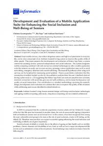
readings produced by different sensors and that the sensor array can coherently differentiate Sensorsmay 2015, be 15, page–page different concentrations, 5 randomly picked sensors were put on calibration runs. This experiment different concentrations, randomly picked sensors were put on calibration runs. exposed This experiment mainly aims to establish the5similarity of readings from different sensors when to the same mainly aims to establish the similarity of readings from different sensors when exposed to the same gas concentrations. gas concentrations. The setup of the calibration system was previously presented by Hawari et al. [30]. In this The setup of the calibration system was previously presented by Hawari et al. [30]. In this experiment, the gas sensor is exposed to different concentrations of ethanol—40, 60, 80, 100 and 120 experiment, the gas sensor is exposed to different concentrations of ethanol—40, 60, 80, 100 and ppm.120 The different ethanol gas concentrations were produced by bubbling compressed air in a 5% ppm. The different ethanol gas concentrations were produced by bubbling compressed air in a 5% ˝ C to produce saturated ethanol gas. Then, by mixing the saturated solution of ethanol in water at at 3030 solution of ethanol in water °C to produce saturated ethanol gas. Then, by mixing the saturated ethanol gas with compressed air, different canbebe reliably produced. ethanol gas with compressed air, differentgas gas concentrations concentrations can reliably produced. AfterAfter initialinitial purgepurge for 300 s, the gasgas sensor is isexposed concentrations ethanol for s. 240 s. After for 300 s, the sensor exposedto toincreasing increasing concentrations of of ethanol gasgas for 240 After concentration, sensorchamber chamberis is purged purged with airair forfor 360360 s to sallow time time for for each each concentration, thethe gasgas sensor withcompressed compressed to allow thesensor gas sensor to return to baseline [31]. the gas to return to baseline [31]. Experiments were standardambient ambient temperature with relative humidity Experiments were runrun ininstandard temperatureand andpressure pressure with relative humidity ranging from 50% to 65%. The sensor response under different calibration profiles is depicted in ranging from 50% to 65%. The sensor response under different calibration profiles is depicted in Figure 10. Table 1 summarizes the steady state readings of all sensors for the three calibration Figure 10. Table 1 summarizes the steady state readings of all sensors for the three calibration profiles. profiles.

Calibration of 5 Gas Sensors 0.7

Sensor Signal, i

0.6 0.5 0.4 0.3 Sensor 1 Sensor 2 Sensor 3 Sensor 4 Sensor 5 3000 3500

0.2 0.1 0 -0.1

0

500

1000

1500 2000 Time,t (s)

2500

(a) Average Sensor Signal 0.8

Sensor Signal, i

0.6

0.4

0.2

0

0

500

1000

1500 Time, t (s)

2000

2500

3000

(b) Gas Sensor Response in Testbed (Row 5) Sensor 1 Sensor 2 Sensor 3 Sensor 4 Sensor 5 Sensor 6

0.35

Sensor Signal, i

0.3 0.25 0.2 0.15 0.1 0.05 0 0

100

200

300

400 500 Time, t (s)

600

700

800

(c) Figure 10. (a) Response of five gas sensors; (b) the average response; and (c) the response of gas

Figure 10. (a) Response of five gas sensors; (b) the average response; and (c) the response of gas sensors in the testbed. sensors in the testbed. 10

30903

Sensors 2015, 15, 30894–30912

In general, all five sensors have the same response when exposed to the same ethanol concentration. The steady state values of all five sensors are similar with small variances and standard Sensors 2015, 15, page–page deviations as presented in Table 1. The data were tested with ANOVA to verify that the different concentration levels can Tableresponse 2, we can conclude thattothe of the In general, all be fivedistinguished. sensors have From the same when exposed thesteady same states ethanol five sensors are similar and that the sensors can differentiate between different concentrations. Hence concentration. The steady state values of all five sensors are similar with small variances and standard as presented 1. The data wereto tested withto ANOVA to accurate verify thatreadings the the gas sensordeviations array operating with in 72Table sensors is expected be able produce different levels be distinguished. From Table provided that concentration all sensors used arecan from the same production lot. 2, we can conclude that the steady states of the five sensors are similar and that the sensors can differentiate between different concentrations. Hence the gas1. sensor array operating with 72 sensors Table Summary of gas sensor calibration results.is expected to be able to produce accurate readings provided that all sensors used are from the same production lot. Sensor

20 ppm

40 ppm

60 ppm

80 ppm

Table 1. Summary of gas sensor calibration results.

100 ppm

Sensor 1 0.6134 0.6677 0.7102 0.7386 0.7558 20 ppm 40 ppm 60 ppm 800.7447 ppm 100 ppm SensorSensor 2 0.6013 0.6728 0.7150 0.7615 SensorSensor 3 0.6018 0.6638 0.7017 0.7303 0.7511 1 0.6134 0.6677 0.7102 0.7386 0.7558 SensorSensor 4 0.6086 0.6698 0.7108 0.7418 0.7631 2 0.6013 0.6728 0.7150 0.7447 0.7615 SensorSensor 5 0.5957 0.6575 0.6914 0.7265 0.7487 3 0.6018 0.6638 0.7017 0.7303 0.7511 Mean 0.6042 0.6663 0.7058 0.7364 0.7560 Sensor 4 0.6086 0.6698 0.7108 0.7418 0.7631 ´5 ´5 ´5 ´5 ´5 Variance 4.7603 ˆ 10 4.7603 ˆ 10 4.7603 ˆ 10 4.7603 ˆ 10 4.7603 Sensor 5 0.5957 0.6575 0.6914 0.7265 0.7487 ˆ 10 Std Dev 0.0061 0.0053 0.0084 0.0069 0.0056 Mean 0.6042 0.6663 0.7058 0.7364 0.7560 Variance 4.7603 × 10−5 4.7603 × 10−5 4.7603 × 10−5 4.7603 × 10−5 4.7603 × 10−5 Table 2. Summary of gas sensor0.0084 calibration results. Std Dev 0.0061 0.0053 0.0069 0.0056 Source of Variation

SS Table 2. Summary df MSsensor calibration F results. of gas

Between Groups 0.073109 SS 4 Source of Variation Within Groups 20 Between Groups0.00108 0.073109 Total 0.074189 24 Within Groups 0.00108 Total 0.074189

338.5219 df0.018277MS F ´5 5.4 ˆ 10 4 0.018277 338.5219 20 5.4 × 10−5 24

p-Value

F crit

4.63 ˆ 10´18 F 2.866081 p-Value crit 4.63 × 10−18 2.866081

3.2. Gas Mapping Using LGSA 3.2. Gas Mapping Using LGSA

Real time monitoring and data storage of mobile olfaction experiments is made possible with the Real time data storage of mobile olfactionfrom experiments made possiblethe with system proposed inmonitoring this paper.and As it was developed separately the otheriscomponents, LGSA the system proposed in this paper. As it was developed separately from the other components, the can be run independently. The gas dispersion in the test bed was recorded using LGSA to study the LGSA can be run independently. The gas dispersion in the test bed was recorded using LGSA to characteristics of gas dispersion in this specific environment. The experiment area and its layout are study the characteristics of gas dispersion in this specific environment. The experiment area and its shownlayout in Figure 11. in Figure 11. are shown

Figure layout thelaboratory laboratory and and picture test area. Figure 11. 11. TheThe layout ofofthe pictureofofthe the test area.

Ethanol is introduced into the environment using a bubbler filled with 20% ethanol solution in

Ethanol is introduced into between the environment bubbler filled with 20% ethanol solution water; with the outlet placed Row 1 andusing Row 2awith coordinates (3, 0.5), marked in Figure 2. in water;Awith the outlet placed between Row 1 and 2 with coordinates (3, 0.5), marked in Figure bladeless fan (Imaha model HTWF Y-12) was Row used to induce air flow when needed. The area was 2. A bladeless fanfrom (Imaha was to induce flow when needed. area closed off any model human HTWF activitiesY-12) during allused experiments. Theair produced airflow in the The testbed is was presented in the following section in Figure 12. closed off from any human activities during all experiments. The produced airflow in the testbed is presented in the following section in Figure 12. 11

30904

Sensors 2015, 15, 30894–30912 Sensors 2015, 15, page–page

The LGSA was lowered to a height of 0.15 m from the testbed platform for all experiments. The air movement in thewas testbed at each sensorofposition wasthe recorded FTTech’s anemometer. The LGSA lowered to a height 0.15 m from testbed with platform for all LM602 experiments. The ˝ The anemometer antestbed air speed resolution of 0.001 and with angleFTTech’s resolution of 0.1 . Each point air movement has in the at each sensor position wasm/s recorded LM602 anemometer. The anemometer has airsamples speed resolution of 0.001 m/sthe and angle resolution of 0.1°. Each point was sampled for 5 min atan five per seconds. Then gas dispersion experiment is conducted wasgas sampled 5 min at five samples per seconds. Then the gas dispersion experiment and all sensorforreadings were recorded. The experiment was run initially with is10conducted min without and all gas sensor readings were recorded. The experiment was run without thea 2 h the wind source or ethanol turned on. Then, the wind source wasinitially turnedwith on 10 formin 5 min before wind source or ethanol turned on. Then, the wind source was turned on for 5 min before a 2 h continuous release of ethanol plume into the testbed. After 2 h, the bubbler was turned off to record continuous release of ethanol plume into the testbed. After 2 h, the bubbler was turned off to record how the air in the testbed clears up after the experiment. To ensure that the gas sensor does not drift, how the air in the testbed clears up after the experiment. To ensure that the gas sensor does not drift, the sensors werewere warmed upup forfor more theexperiments experiments were run. the sensors warmed morethan thanaaweek week before before the were run.

Figure 12. Average airflow in testbed—fan turned on.

Figure 12. Average airflow in testbed—fan turned on.

This section will describe and discuss the data collected from the LGSA from the experiment runs.

This sectionacknowledge will describethat and discuss the data collected from fromofthe The authors three-dimension air movement affectsthe theLGSA dispersion gasexperiment in the however this paper will only consider gas dispersion along a affects 2-D plane to of 2-D runs.testbed; The authors acknowledge that three-dimension air movement thepertaining dispersion gas in mobile olfaction strategies. The 2-D information provided by the system is adequate for the development the testbed; however this paper will only consider gas dispersion along a 2-D plane pertaining to of 2-D mobile olfaction strategies as the would only traverse in 2-D space. 2-D mobile olfaction strategies. The 2-Drobot information provided bya the system is adequate for the development of 2-D mobile olfaction strategies as the robot would only traverse in a 2-D space. 3.2.1. Airflow Produced in the Testbed

3.2.1. Airflow Produced of in odor the Testbed The dispersion is heavily influenced by the advection and diffusion of the gas the carrying fluid. Therefore, the air movement in the testbed is measured and studied first to

The dispersion of odor is heavily influenced by the advection and diffusion of the gas the understand the gas plume structure produced. The recorded air movement in the testbed is shown carrying fluid.12; Therefore, air movement in the is testbed is measured studied to understand in Figure however, the the natural air movement prevalent downwindand (at the top offirst Figure 12). As the gas plume structure produced. Thewind recorded movement thecm/s testbed shown Figure 12; there is induced airflow, the average speedair is on average = in 41.0 ± 41.5iscm/s withinairflow however, natural is prevalent downwind the are topalso of “dead Figurezones”—areas 12). As there is speedthe ranging fromair 9.2movement cm/s ± 5.3 cm/s to 214.8 cm/s ± 10.8 cm/s.(at There withairflow, relatively low airflow,wind wherespeed the induced airflow meets with the ˘ natural airflow. induced the average is on average = 41.0 cm/s 41.5 cm/s with airflow speed The variation considered dividing airflow vectors into“dead 1° direction bins, ranging from 9.2 cm/sof˘the 5.3airflow cm/s was to 214.8 cm/s by ˘ 10.8 cm/s. There are also zones”—areas summing magnitude theinduced airflow vectors each with bin. Interestingly, the distribution of with and relatively lowthe airflow, whereofthe airflowin meets the natural airflow. airflow was observed fit a one term Gaussian distribution forairflow most positions this1experimental ˝ direction bins, The variation of the to airflow was considered by dividing vectorsininto setup. The points where the distribution deviates from Gaussian distribution is when there are and summing the magnitude of the airflow vectors in each bin. Interestingly, the distribution of obstacle nearby or when the airspeed is very low. A graphical description of the airflow distribution airflow was observed to fit a one term Gaussian distribution for most positions in this experimental setup. The points where the distribution deviates 12 from Gaussian distribution is when there are obstacle nearby or when the airspeed is very low. A graphical description of the airflow distribution 30905

Sensors 2015, 15, 30894–30912 Sensors 2015, 15, page–page

is shown Figure 13. The data collected in this testbed verify the assumption in odor dispersion Sensorsin 2015, 15, page–page is shown in Figure 13. The data collected in this testbed verify the assumption in odor dispersion models that the variations in air speed and direction fit to the Gaussian distribution.

of Magnitude Sum of Sum Magnitude (m/s) (m/s)

0 100 150

of Magnitude Sum of Sum Magnitude (m/s) (m/s)

Airflow Data Fitted Curve Airflow Data Fitted Curve

120

140 160 Direction ( )

120

140 160 Direction ( )

150 100

180

200

180

200

Airflow Data Fitted Curve Airflow Data Fitted Curve

100 50 50 0 130

of Magnitude Sum of Sum Magnitude (m/s) (m/s)

0 130 25 20 25 15 20 10 15 5 10 0 170 5 0 170

150 150

170 190 Direction ( ) 170 190 Direction ( )

210 210

230

190 190

210 230 Direction ( ) 210

230

250 250

50 100

230

Airflow Data Fitted Curve

270 270

Airflow Data Fitted Curve

100 150

0 50 120

140

160 180 Direction ( )

0 120 60

140

160 180 Direction ( )

60 40

200

220

200

220

Airflow Data Fitted Curve Airflow Data Fitted Curve

40 20 20 0 150 0 150 50

Airflow Data Fitted Curve

Airflow Data Fitted Curve

150 200

of Magnitude Sum of Sum Magnitude (m/s) (m/s)

80 100 60 80 40 60 20 40 0 100 20

of Magnitude Sum of Sum Magnitude (m/s) (m/s)

of Magnitude Sum of Sum Magnitude (m/s) (m/s)

models that the variations in air speed and direction fit to the Gaussian distribution. is shown in Figure 13. The data collected in this testbed verify the assumption in odor dispersion models that the 100 variations in air speed and direction fit 200to the Gaussian distribution.

170

190 210 Direction ( )

170

190 210 Direction ( )

230

250

230

250

Airflow Data Fitted Curve

40 50 30 40 20 30 10 20 0 160 10

180

200 220 Direction ( )

240

260

0 160

180

200

240

260

Airflow Data Fitted Curve

220

Direction (13.  ) Distribution of airflow in the testbed. Direction ( ) Figure

Figure 13. Distribution of airflow in the testbed.

3.2.2. Gas Dispersion

Figure 13. Distribution of airflow in the testbed.

3.2.2. Gas Dispersion

dispersion in the testbed agrees with the measured airflow. The gas was distributed 3.2.2.The Gasaverage Dispersion

The in thethe testbed agrees with14. the measured airflow. Themap gas was distributed alongaverage the maindispersion airflow towards bottom of Figure The average concentration agrees with The average dispersion in the testbed agrees with the measured airflow. The gas was distributed most of the instantaneous concentration maps during the experiment. However, there are still alongalong the main airflow bottomofofFigure Figure The average concentration map agrees the main airflowtowards towards the the bottom 14. 14. The average concentration map agrees with differences in the instantaneous concentration maps as compared to the averaged concentration map. with most most of of the instantaneous concentration maps during the experiment. However, there are the instantaneous concentration maps during the experiment. However, there are still still differences in instantaneous maps compared toaveraged the averaged concentration differencesthe in the instantaneousconcentration concentration maps asas compared to the concentration map. map.

Figure 14. Average gas distribution map in testbed. The estimated ethanol concentration is described on the color scale. Figure 14. Average distribution mapinintestbed. testbed. The concentration is described Figure 14. Average gasgas distribution map Theestimated estimatedethanol ethanol concentration is described 13 on the color scale. on the color scale.

13

30906

Sensors 2015, 15, 30894–30912 Sensors 2015, 15, page–page

The target target gas was released into the s. One minute after the The the testbed testbed between betweentt==900 900s stotot =t 8100 = 8100 s. One minute after gasgas waswas released, the the detected plume resembles the average plume in terms of shape, although with the released, detected plume resembles the average plume in terms of shape, although lowerlower concentrations. The The plume keeps its its shape and increases the with concentrations. plume keeps shape and increasesininconcentration concentrationas as shown shown in the concentration map map at at t == 1500 ofof gas in concentration 1500 s.s.As Asthe theexperiment experimentcontinues, continues,there thereappears appearstotobebea build-up a build-up gas thethe testbed. At At t = t2700 s, although the main plume maintains the same shape, the surrounding area in testbed. = 2700 s, although the main plume maintains the same shape, the surrounding around the main plume records increased gas gas concentrations. TheThe accumulation of the gas gas andand the area around the main plume records increased concentrations. accumulation of the variability in the contributes to the in theingeneral shapeshape of the of gasthe plume as shown the variability in airflow the airflow contributes tovariability the variability the general gas plume as in the series of snapshots in Figure 15. It is worth noting that the area around the main plume shown in the series of snapshots in Figure 15. It is worth noting that the area around the plume accumulated significant significantlevels levelsof ofgas gasuntil untilthe thegas gasflow flowwas wasstopped stoppedatattt== 8100 8100s.s. After After the the gas gas flow flow accumulated was stopped, stopped, the the concentration concentrationlevels levelsin inthe thetestbed testbeddecreases decreasesuntil untilititclears clearsup upatattt==11,700 11,700s.s. was

Figure 15. Snapshot of gas distribution map in testbed; (a) t = 900 s; (b) t = 960 s; (c) t = 1500 s; Figure 15. Snapshot of gas distribution map in testbed; (a) t = 900 s; (b) t = 960 s; (c) t = 1500 s; (d) t = 2700 s; (e) t = 4700 s and (f) t = 6400 s. The estimated ethanol concentration is described on the (d) t = 2700 s; (e) t = 4700 s and (f) t = 6400 s. The estimated ethanol concentration is described on the color scale. color scale.

The The instantaneous instantaneous gas gas dispersion dispersion shows shows that that on on average, average, gas gas usually usually disperses disperses in in the the general general direction of the airflow through advection. However, the instantaneous gas dispersion can deviate direction of the airflow through advection. However, the instantaneous gas dispersion can deviate far far from from the the average average gas gas dispersion dispersion map map due due to to variation variation in in airflow. airflow. The The LGSA LGSA was was able able to to capture capture the the instantaneous instantaneous dispersion dispersionof ofthe thegas gasin inthis thisexperiment. experiment. 3.3. Gas Mapping Using LGSA 3.3. Gas Mapping Using LGSA Two sets of mobile olfaction experiments were conducted to gauge the performance of the LGSA Two sets of mobile olfaction experiments were conducted to gauge the performance of the by recreating the experiment as described in the previous section. The setup was chosen as it creates a LGSA by recreating the experiment as described in the previous section. The setup was chosen as it relatively stable gas plume profile. The gas concentration measurements made by a robot is compared creates a relatively stable gas plume profile. The gas concentration measurements made by a robot is with the LGSA measurements. The robot used was a remote controlled National Instrument Robotics compared with the LGSA measurements. The robot used was a remote controlled National Instrument Robotics sbRIO Kit 2.0 equipped with a TGS2600 gas sensor. The gas sensor was placed 30907 14

Sensors 2015, 15, 30894–30912

Sensors 2015, 15, page–page

sbRIO Kit 2.0 equipped with a TGS2600 gas sensor. The gas sensor was placed at the highest point of the robot (approximately cm from the ground)19such that the sensorsuch on the at sensor the same at the highest point of the19 robot (approximately cm from thegas ground) thatroot the is gas on height LGSA. Similarly, thethe LGSA was lowered the to aLGSA heightwas of 19 cm from ground. the rootasisthe at the same height as LGSA. Similarly, lowered to athe height of 19The cm robot’s trajectory depicted Figures 16 and 17. in Figures 16 and 17. from the ground. is The robot’sintrajectory is depicted The first gas distribution measurement The first gas distribution measurement was was made made by by aa constantly constantly moving moving robot robot in in the the testbed testbed area. area. In In the the second second experiment, experiment, the the robot robot stops stops for for 55 ss when when taking taking gas gas concentration concentration measurements. measurements. In In both both experiments, experiments, the the LGSA LGSA was was used used to to monitor monitor the the gas gas concentration concentration in in the the testbed. testbed. In In this this section, section, the the gas gas concentration concentration maps maps for for the the robots robots are are interpolated interpolated by by triangulation. triangulation. Contour Contour maps maps are are used used to to better better depict depict the the concentration concentration levels levels and and the the shape shape of of the the gas gas plume. plume. Robot Gas Mapping 6

5

5

4

4

y (m)

y (m)

Average Gas Dispersion in Testbed 6

3

3

2

2

1

1

0

0

1

2

0

3

x (m)

0

1

2

(a)

(b)

Estimated Average Reading from LGSA

Estimated Reading from Real-time LGSA 6

5

5

4

4

y (m)

y (m)

6

3

3

2

2

1

1

0

3

x (m)

0

0

1

2

0

1

3

2

3

x (m)

x (m)

(c)

(d)

Figure 16. Gas distribution plots of constantly moving robot experiment. The robot’s movement path Figure 16. Gas distribution plots of constantly moving robot experiment. The robot’s movement is denoted by the line and the dots indicate measurement points. The robot starts at the top right path is denoted by the line and the dots indicate measurement points. The robot starts at the corner of the map. (a) The averaged LGSA reading for the duration of the experiment; (b) The top right corner of the map. (a) The averaged LGSA reading for the duration of the experiment; measured gas concentration by the robot; (c) The ground truth robot reading estimated from the (b) The measured gas concentration by the robot; (c) The ground truth robot reading estimated from averaged LGSA measurement; (d) The ground truth robot reading estimated from the real-time the averaged LGSA measurement; (d) The ground truth robot reading estimated from the real-time LGSA measurements. measurements. LGSA

As the gas sensor is slow, the gas concentration measurement made by the moving robot appears to be distorted compared to the averaged gas concentration. The gas sensor was unable to reach steady state as the robot was moving. The delay is obvious if the map is compared with Figure 16d, which is the expected gas measurement if30908 the gas sensor response is ideally fast. Furthermore, 15

Sensors 2015, 15, 30894–30912

As the gas sensor is slow, the gas concentration measurement made by the moving robot appears to be distorted compared to the averaged gas concentration. The gas sensor was unable to reach steady state as the robot was moving. The delay is obvious if the map is compared with Figure 16d, 2015, 15, page–page whichSensors is the expected gas measurement if the gas sensor response is ideally fast. Furthermore, the gas sensor signal increases and decreases slower and the peaks and troughs are detected at delayed the gas sensor signal increases and decreases slower and the peaks and troughs are detected at positions; skewing the concentration maps. If the sensor was sufficiently fast and more data were delayed positions; skewing the concentration maps. If the sensor was sufficiently fast and more data sampled at each points, the gas concentration map produced would be similar to Figure 16c. To were sampled at each points, the gas concentration map produced would be similar to Figure 16c. To demonstrate thisthis point, a second run with withthe therobot robot stopping while making demonstrate point, a secondexperiment experiment was was run stopping while making gas gas concentration measurements. concentration measurements. Robot Gas Mapping 6

5

5

4

4

y (m)

y (m)

Average Gas Dispersion in Testbed 6

3

3

2

2

1

1

0

0

1

2

0

3

x (m)

0

1

(a)

5

5

4

4

y (m)

y (m)

Estimated Reading from Real-time LGSA 6

3

3

2

2

1

1

0

1

3

(b)

Estimated Average Reading from LGSA 6

0

2 x (m)

2

3

0

0

1

x (m)

2

3

x (m)

(c)

(d)

Figure 17. Gas distribution plots of stop–start robot experiment. The robot’s movement path is

Figure 17. Gas distribution of stop–start robot point. experiment. robot’s movement path is denoted by the line and theplots dots indicate measurement The robotThe starts at the top right corner denoted by the line and the dots indicate measurement point. The robot starts at the top right corner of the map. (a) The averaged LGSA reading for the duration of the experiment; (b) The measured gas of theconcentration map. (a) Thebyaveraged LGSA reading for the duration of the experiment; (b) The measured the robot; (c) The ground truth robot reading estimated from the averaged LGSA gas measurement; (d)robot; The (c) ground truth robot reading estimated from from the real-time LGSA concentration by the The ground truth robot reading estimated the averaged LGSA measurements. measurement; (d) The ground truth robot reading estimated from the real-time LGSA measurements.

The stop–start measurement method produces a gas concentration map which is much closer to the time-averaged gas concentration map and reveals an obvious gas plume seen in Figure 17b.

30909 16

Sensors 2015, 15, 30894–30912

The stop–start measurement method produces a gas concentration map which is much closer to the time-averaged gas concentration map and reveals an obvious gas plume seen in Figure 17b. Even though the robot stops for 5 s while measuring the gas concentration, the robot was still unable to properly measure either the time-averaged or the instantaneous gas concentration levels. As such, similar distortions seen in the map created by a constantly moving robot is seen in the stop–start measurement; albeit less prominently. It is known that the robot affects the air movement in the testbed, and thus the gas dispersion in the testbed. However, no changes in the gas dispersion maps which can be attributed to the presence of the robot was observed. This may be due to the variability of the gas dispersion itself masking the effects of the robots presence. Furthermore, as the gas sensor on the robot and the LGSA is located higher than the bulk size of the robot, it is possible that the presence of the robot minimally affects the gas dispersion at the height of the gas sensors. The high net airflow at the gas sensors’ level may explain this phenomena. This experiment will not be pursued further in this document; however it has proven the need of ground truth knowledge to fully optimize and verify a mobile olfaction system. 4. Conclusions In this work, a scalable system for mobile olfaction experimentation based on WSN backbone has been presented. Sensor calibration has verified that a large array of sensors can produce coherent sensor signals provided that the sensors are from the same production lot. The main component of the system, the LGSA, has been shown to be able to provide snapshots of the gas dispersion in the testbed which may aid to the design and test process of a mobile olfaction system. In addition, the collected results have shown the variability and the unpredictability in the gas dispersion, which information is lost in a time-averaged gas dispersion map. Furthermore, the system has demonstrated its usefulness in verifying the results of a gas distribution mapping experiment. Further work includes improvements in gas distribution map plotting to create more accurate representation where various offline models have been proposed [32]. The gas sensor array may also be improved by increasing the number of sensor and integrating newer gas sensors which is faster, smaller in size and more energy efficient (e.g., MiCS-5526 or CCMOS CCS803 VOC sensor). It is envisaged that, with faster and more sensitive sensors, more variations in the gas plume may be observed thus providing better insight to the mobile olfaction problem. It is also possible to change the configuration of the LGSA to detect different types of gas by simply changing the gas sensors. However, as some types of gas sensors are slow and have relatively slower recovery times, the performance of the LGSA may differ depending on the types of gas sensor used. Acknowledgments: The authors wish to express their gratitude to the Malaysian Ministry of Education for their scholarship for Syed Muhammad Mamduh and Kamarulzaman Kamarudin. Author Contributions: In this paper, Syed Muhammad Mamduh and Retnam Visvanathan contributed in the system development, experimental work and manuscript writing. Kamarulzaman Kamarudin, Ahmad Shakaff Ali Yeon contributed in the data analysis, and manuscript writing. Ali Yeon Md. Shakaff Ammar Zakaria and Latifah Munirah Kamarudin contributed in experiment design, data analysis and manuscript writing. Conflicts of Interest: The authors declare no conflict of interest.

References 1. 2.

3.

Marques, L.; de Almeida, A.l.T. Application of Odor Sensors in Mobile Robotics. In Autonomous Robotic Systems; de Almeida, A., Khatib, O., Eds.; Springer: London, UK, 1998; pp. 82–95. Russell, A.; Thiel, D.; Mackay-Sim, A. Sensing Odour Trails for Mobile Robot Navigation. In Proceedings of the 1994 IEEE International Conference on the Robotics and Automation, San Diego, CA, USA, 8–13 May 1994; pp. 2672–2677. Marjovi, A.; Marques, L. Multi-Robot Odor Distribution Mapping in Realistic Time-Variant Conditions. In Proceedings of the 2014 IEEE International Conference on Robotics and Automation (ICRA), Hong Kong, China, 31 May–7 June 2014; pp. 3720–3727.

30910

Sensors 2015, 15, 30894–30912

4.

5.

6.

7. 8. 9. 10. 11.

12.

13.

14.

15. 16.

17.

18.

19. 20.

21.

22.

Wu, Y.-X.; Meng, Q.-H.; Zhang, Y.; Zeng, M. A Novel Chemical Plume Tracing Method Using a Mobile Sensor Network Without Anemometers Mechanical Engineering and Technology; Zhang, T., Ed.; Springer: Berlin/Heidelberg, Germany, 2012; pp. 155–162. Zhang, J.; Zhang, X.; Sun, L.; Zhu, M. Basing on the Olfaction and Vision Information Fusion for Robot's Odor Source Localization. In Proceedings of the 2010 IEEE International Conference on Robotics and Biomimetics (ROBIO), Tianjin, China, 14–18 December 2010; pp. 845–849. Marques, L. Good Experimental Methodologies for Mobile Robot Olfaction. In Proceedings of the Robotics: Science and Systems Conference (RSS2009), Workshop on Good Experimental Methodology in Robotics, Seattle, WA, USA, 28 June–1 July 2009; pp. 291–294. Farrell, J.A.; Murlis, J.; Long, X.; Li, W.; Cardé, R.T. Filament-based atmospheric dispersion model to achieve short time-scale structure of odor plumes. Environ. Fluid Mech. 2002, 2, 143–169. [CrossRef] Hayes, A.T.; Martinoli, A.; Goodman, R.M. Swarm robotic odor localization: Off-line optimization and validation with real robots. Robotica 2003, 21, 427–441. [CrossRef] Martinez, D.; Rochel, O.; Hugues, E. A biomimetic robot for tracking specific odors in turbulent plumes. Auton. Robots 2006, 20, 185–195. [CrossRef] Marjovi, A.; Marques, L. Optimal spatial formation of swarm robotic gas sensors in odor plume finding. Auton. Robots 2013, 35, 93–109. [CrossRef] Ramirez, A.R.G.; Lopez, A.L.; Rodriguez, A.B.; de Albornoz, A.D.C.; de Pieri, E.R. An Infotaxis Based Odor Navigation Approach. In Proceedings of the Biosignals and Biorobotics Conference (BRC), 2011 ISSNIP, Vitoria, Brazil, 6–8 January 2011; pp. 1–6. Neumann, P.; Bennetts, V.H.; Lilienthal, A.J.; Bartholmai, M. From insects to micro air vehicles: A comparison of reactive plume tracking strategies. In Proceedings of the 13th International Conference on Intelligent Autonomous Systems, Padova, Italy, 15–19 July 2014; pp. 1–12. Bennetts, V.H.; Lilienthal, A.J.; Schaffernicht, E.; Ferrari, S.; Albertson, J. Integrated simulation of gas dispersion and mobile sensing systems. In Proceedings of the Workshop on Realistic, Rapid and Repeatable Robot Simulation (R4SIM), Robotics: Science and Systems XI, Rome, Italy, 16 June 2015. Cabrita, G.; Sousa, P.; Marques, L. Player/stage simulation of olfactory experiments. In Proceedings of the 2010 IEEE/RSJ International Conference on Intelligent Robots and Systems (IROS), Taipei, Taiwan, 18–22 October 2010; pp. 1120–1125. Ishida, H.; Kagawa, Y.; Nakamoto, T.; Moriizumi, T. Odor-source localization in the clean room by an autonomous mobile sensing system. Sens. Actuators B Chem. 1996, 33, 115–121. [CrossRef] Purnamadjaja, A.H.; Russell, R.A. Pheromone Communication: Implementation of Necrophoric Bee Behaviour in a Robot Swarm. In Proceedings of the 2004 IEEE Conference on the Robotics, Automation and Mechatronics, Singapore, 1–3 December 2004; pp. 638–643. Pyk, P.; Bermúdez i Badia, S.; Bernardet, U.; Knüsel, P.; Carlsson, M.; Gu, J.; Chanie, E.; Hansson, B.; Pearce, T.J.; Verschure, P.M. An artificial moth: Chemical source localization using a robot based neuronal model of moth optomotor anemotactic search. Auton. Robots 2006, 20, 197–213. [CrossRef] Lilienthal, A.; Reggente, M.; Trincavelli, M.; Blanco, J.L.; Gonzalez, J. A statistical approach to gas distribution modelling with mobile robots—The kernel dm+v algorithm. In Proceedings of the IEEE/RSJ International Conference on Intelligent Robots and Systems, 2009, IROS 2009, St. Louis, MO, USA, 10–15 October 2009; pp. 570–576. Hayes, A.T.; Martinoli, A.; Goodman, R.M. Distributed odor source localization. IEEE Sens. J. 2002, 2, 260–271. [CrossRef] Akat, S.B.; Gazi, V.; Marques, L. Asynchronous particle swarm optimization-based search with a multi-robot system: Simulation and implementation on a real robotic system. Turkish J. Electr. Eng. Comput. Sci. 2010, 18, 749–764. Vergara, A.; Fonollosa, J.; Mahiques, J.; Trincavelli, M.; Rulkov, N.; Huerta, R. On the performance of gas sensor arrays in open sampling systems using inhibitory support vector machines. Sens. Actuators B Chem. 2013, 185, 462–477. [CrossRef] Fonollosa, J.; Rodríguez-Luján, I.; Trincavelli, M.; Vergara, A.; Huerta, R. Chemical discrimination in turbulent gas mixtures with mox sensors validated by gas chromatography-mass spectrometry. Sensors 2014, 14, 19336–19353. [CrossRef] [PubMed]

30911

Sensors 2015, 15, 30894–30912

23.

24.

25.

26. 27.

28.

29. 30.

31.

32.

Jatmiko, W.; Sekiyama, K.; Fukuda, T. A pso-based mobile robot for odor source localization in dynamic advection-diffusion with obstacles environment: Theory, simulation and measurement. IEEE Computat. Intell. Mag. 2007, 2, 37–51. [CrossRef] Ishida, H. Robotic systems for gas/odor source localization: Gap between experiments and real-life situations. In Proceedings of the IEEE International Conference on Robotics and Automation (ICRA 2007), Roma, Italy, 10–14 April 2007; pp. 3–8. Marjovi, A.; Marques, L. Swarm robotic plume tracking for intermittent and time-variant odor dispersion. In Proceeding of the 2013 European Conference on Mobile Robots (ECMR), Barcelona, Spain, 25–27 September 2013; pp. 379–384. Cabrita, G.; de Sousa, P.A.M.; Marques, L. Odor Guided Exploration and Plume Tracking-Particle Plume Explorer; ECMR: Örebro, Sweden, 2011. Pomareda, V.; Hernández, V.; Khaliq, A.A.; Trincavelli, M.; Lilienthal, A.J.; Marco, S. Chemical source localization in real environments integrating chemical concentrations in a probabilistic plume mapping approach. In Proceedings of the 15th International Symposium on Olfaction and Electronic Nose, ISOEN, Daegu, Korea, 2–5 July 2013; pp. 587–588. Mamduh, S.M.; Kamarudin, K.; Saad, S.M.; Shakaff, A.Y.M.; Zakaria, A.; Abdullah, A.H. Braitenberg swarm vehicles for odour plume tracking in laminar airflow. In Proceedings of the 2013 IEEE Symposium on Computers & Informatics (ISCI), Langkawi, Malaysia, 7–9 April 2013; pp. 1–6. Gonzalez-Jimenez, J.; Monroy, J.G.; Blanco, J.L. The multi-chamber electronic nose—An improved olfaction sensor for mobile robotics. Sensors 2011, 11, 6145–6164. [CrossRef] [PubMed] Hawari, H.F.; Samsudin, N.M.; Shakaff, A.Y.M.; Wahab, Y.; Hashim, U.; Zakaria, A.; Ghani, S.A.; Ahmad, M.N. Highly selective molecular imprinted polymer (mip) based sensor array using interdigitated electrode (ide) platform for detection of mango ripeness. Sens. Actuators B Chem. 2013, 187, 434–444. [CrossRef] Kamarudin, K.; Mamduh, S.M.; Md Shakaff, A.Y.; Mad Saad, S.; Zakaria, A.; Abdullah, A.H.; Kamarudin, L.M. Flexible and autonomous integrated system for characterizing metal oxide gas sensor response in dynamic environment. Instrum. Sci. Technol. 2015, 43, 74–88. [CrossRef] Reggente, M.; Lilienthal, A. The 3d-kernel dm+v/w algorithm: Using wind information in three dimensional gas distribution modelling with a mobile robot. In Proceedings of the 2010 IEEE Sensors, Kona, HI, USA, 1–4 November 2010; pp. 999–1004. © 2015 by the authors; licensee MDPI, Basel, Switzerland. This article is an open access article distributed under the terms and conditions of the Creative Commons by Attribution (CC-BY) license (http://creativecommons.org/licenses/by/4.0/).

30912