DEVELOPMENT OF A SYSTEM FOR DETERMINING COLLECTION EFFICIENCY OF SPRAY SAMPLERS B. K. Fritz, W. C. Hoffmann ABSTRACT. A methodology for evaluating the collection efficiency (CE) of airborne spray flux samplers in a low speed spray dispersion tunnel was developed and evaluated. Prior to evaluation of the testing protocol, dispersion tunnel operating characteristics were examined. Air speeds and flux measurements in the working section of the tunnel showed defined gradients which the collection efficiency protocol had to address. The proposed methodology used soda straws and monofilament line as spray flux samplers because their theoretical CE could be calculated to estimate the actual spray flux measured across a sampler of interest. This estimated actual flux was then used to determine the experimental collection efficiency of this sampler. This protocol was tested by comparing the theoretically and experimentally derived CE of soda straw collectors. Results showed no statistical difference between the theoretical and experimental CE at each air speed tested. As the air speeds increased from 0.45 to 4.0 m/s, the CE for the monofilament line increased from 52.3% to 82.6%, respectively, while the CE of the soda straw also increased from 6.7% to 45%, respectively. This methodology might be used to determine CE for various spray flux samplers, such as flat plate collectors, rotating rods, and screens. Keywords. Collection efficiency, Spray sampling, Spray application, Spray flux measurement.
M
ovement of sprays within and off of target areas is a critical concern for applicators, neighboring landowners, and researchers. Ideally, all of the material applied should be deposited within the targeted swath on the targeted pest or crop. Realistically, some portion of the spray remains airborne and is carried downwind. Airborne spray leaving the targeted area reduces the applied dosage and could create unintended crop or plant damage. It could also cause hazards or other detrimental environmental impacts. The measurement and quantification of the airborne spray is difficult. Researchers have used passive collection media such as cotton string or cord (Whitney and Roth, 1985; Fox et al., 1990, 1993; SDTF, 1994), nylon string (Kirk, 1999; Fritz, 2006), various flat tapes (Fox et al., 1990, 1993; SDTF, 1994), soda straws (Fritz et al., 2006), and wire (Riley and Wiesner, 1990) to measured spray flux, which is the amount of spray that passes through an area. Several active samplers have been reported including rotating impactors (Lesnic et al, 1993; Kramer and Schutz, 1994; Cooper et al., 1996) and isokenetic samplers (Bui et al., 1998). Collection efficiency (CE) is defined as the fraction of spray droplets approaching a surface or collector that actually deposits on that surface. Due to the unique shape and physical characteristics of the different samplers/collectors, each has a unique CE which is
Submitted for review in July 2007 as manuscript number PM 7074; approved for publication by the Power & Machinery Division of ASABE in January 2008. Mention of a commercial or proprietary product does not constitute an endorsement for its use by the U.S. Department of Agriculture. The authors are Bradley K. Fritz, ASABE Member Engineer, Agricultural Engineer and Clint Hoffmann, ASABE Member Engineer, Agricultural Engineer, USDA‐ARS, College Station, Texas. Corresponding author: Bradley K. Fritz, USDA‐ARS, 2771 F&B Rd., College Station, TX 77845; phone: 979‐260‐9584; fax: 979‐260‐9386; e‐mail:
[email protected].
dependent on droplet size and wind speed. The active samplers are further complicated when the sampling rate differs from the aspiration rate (Cooper at al., 1996). Additionally, the rotary samplers and the “fuzzy” line samplers (i.e. cotton cord and pipe cleaners) have a collection area that is somewhat ambiguous. Without knowing the CE of the collectors used in a study, it is difficult to interpret the collected data and compare with other studies that used different collectors or comparing the collected data to modeled data. The theoretical CEs of droplets on cylindrical, spherical, long ribbon, and disc‐shaped collectors were measured and reported by May and Clifford (1967). Their research examined the impaction of 20‐, 30‐, and 40‐μm droplets of dibutyl phthalate (density of 1 g/m3) on spheres (2.65‐, 1.27‐, 1.05‐, 0.475‐, and 0.158‐cm diameters), discs (2.875, 1.431‐, 0.995‐, 0.485‐, and 0.154‐diameters), cylinders (1.965‐, 1.430‐, 0.992‐, 0.475‐, and 0.125‐cm diameters), and ribbons (1.9‐, 1.265‐, 0.8‐, 0.13‐, and 0.1045‐cm widths) under air speeds of 2.2, 3.1, 4.5, and 6.2 m/s. They found that their measured efficiencies for cylindrical collectors agreed with theoretical calculations of Langmuir and Blodgett (1944, as reported in May and Clifford, 1967). An equation fit to the May and Clifford (1967) data for cylinders is presented and used in this research. Not all collectors fit these ideal shapes and thus require experimental determination. Researchers have used a number of methodologies for CE evaluations including testing and exposure under ambient field conditions (Bui et al., 1998; Salyai et al., 2006) to small‐scale wind tunnels (May and Clifford, 1967; Cooper et al., 1996; Fox et al., 2004) and mathematical and computer modeling (Lesnic et al., 1993; Kramer and Schutz, 1994; Zhu et al., 1996). The work herein describes a methodology for evaluating CE using a combination of small‐scale wind tunnel and mathematical evaluations. The objective of this research was to develop and evaluate a methodology for evaluating the CE of passive airborne
Applied Engineering in Agriculture Vol. 24(3): 285‐293
2008 American Society of Agricultural and Biological Engineers ISSN 0883-8542
285
spray flux samplers using a small‐scale, low air speed, dispersion tunnel.
MATERIALS AND METHODS A low air speed, spray dispersion tunnel with a mixing chamber was constructed for use in airborne spray sampler passive collector CE studies (fig. 1). Prior to the CE evaluations, the tunnel operating characteristics and performance was evaluated. The primary area of concern was the profile of the spray droplet size spectra and the spray flux across the cross‐sectional area of the tunnel, where collectors were to be positioned. After evaluation of the tunnels inherent dispersion characteristics, i.e. the flux profiles under the selected operating parameters, was completed, a CE evaluation protocol was tested using ideal collectors (where an ideal collector is a collector whose CE can be determined theoretically). The passive collectors used in this study were soda straws and monofilament line. These were chosen due to their extensive use the authors' other research efforts, as well as, for their cylindrical shape allowing for the calculation of the theoretical CE. SPRAY DISPERSION TUNNEL CONSTRUCTION The constructed low speed dispersion tunnel's cross‐sectional area was 0.9 × 0.9 m. The tunnel consists of a 2.4‐m long entry section at the beginning of which a spray nozzle is mounted. The entry section enters into a 1.8‐ × 1.8‐ × 3.7‐m mixing chamber. A 4.9‐m long section, also 0.9 × 0.9 m, exits the mixing chamber. A flow straightener consisting of a 5‐ × 5‐cm grided square section 0.75 m in length was placed in the 0.9‐ × 0.9‐ × 2.4‐m section between the fan inlet and the sampler location. A fan pulls air through the system (fig. 1). Airspeed in the tunnel was varied by adjusting an inline gate valve. Minimum and maximum mean air speeds in the tunnel are 0.2 and 5.4 m/s, respectively. During all measurements, samplers were located in the center of the last 2.4‐m section before the fan (fig. 1). An access panel allowed for the placement and recovery of collectors (fig. 1). Additionally, two holes were cut (centered vertically on the walls), on each opposing wall, 1.8‐m
upstream of the test section allowed access (fig. 1) of a Sympatec HELOS laser diffraction droplet sizing system (Sympatec Inc., Clausthal, Germany). Spray was released into the tunnel using an air assisted nozzle (Advanced Special Technologies, Winnebago, Minn.). The dual venturi style, stainless steel nozzle was designed to be used on the Terminator ULV Sprayer (Advanced Special Technologies, Winnebago, Minn.). Hoffmann et al. (2007) reported average droplet volume median diameters of 20.4 and 21.7 mm for water‐based and oil sprays, respectively. For this work, the spray nozzle was removed from the Terminator sprayer and connected to a compressor with a pressure regulator inline. The self‐feed tube from the nozzle was attached to an inline flow meter. This allowed for a metered material release to the spray nozzle. The nozzle was operated at 689 kPa (100 psi) and fed 10 mL of Orchex 796 mineral oil (Calumet Lubricants Co., L.P., Indianapolis, Ind.) with Uvitex fluorescent dye at the rate of 1g/L of oil. DROPLET SIZING A Sympatec Helos laser diffraction droplet sizing system (Sympatec Inc., Clausthal, Germany) was used to measure droplet size data. The Helos system uses a 623‐nm He‐Ne laser and was fitted with an R5 lens, which resulted in a dynamic size range of 0.5 to 875 mm in 32 sizing bins. Tests were performed within the guidelines provided by ASTM Standard E1260: Standard Test Method for Determining Liquid Drop Size Characteristics in a Spray Using Optical Nonimaging Light‐Scattering Instruments (ASTM, 2003). Droplet sizing data measured included volume median diameter (DV50), the 10% and 90% diameters (DV10 and DV90), the relative span (RS), and the percent volume less the 100 mm (ASTM, 1997). AIR VELOCITY MEASUREMENTS Prior to any flux measurements, air velocity measurements were made at the location where sample media would be placed during the CE evaluations. Following the International Standards Organization's (ISO) Draft Standard 22856 recommendations (ISO, 2005),
Figure 1. Spray dispersion tunnel with locations of spray nozzle, Sympatec HELOS laser diffraction system, sampler placement, and flow straightener locations indicated.
286
APPLIED ENGINEERING IN AGRICULTURE
measurements were taken at nine evenly spaced locations (three rows of three points in 22.9‐cm increments) using a hot‐wire anemometer (Extech Instruments, Model 407119A, Waltham, Mass.). The hot‐wire anemometer had an effective range for air velocity of 0.2 to 17.0 m/s with a resolution of 0.1 m/s and a stated accuracy of ±5%. One dimensional velocity (along the axis of the wind tunnel) measurements in each location were recorded every second (minimum interval of the anemometer) over a 2‐min period. Measurements were made with the wind tunnel operating at mean airspeeds of 0.45, 2.2, and 4.0 m/s. Recorded data were analyzed and air speed means and standard deviations at each location and for each air speed were determined. The air speed during the flux profiling and the CE work was collected using the hot‐wire anemometer positioned in the center of the tunnel's cross‐sectional area. The air speeds selected are a function of tunnel limitations as well as meant to be representative of typical field conditions where measurements are made. FLUX PROFILE EVALUATION The flux profile through the tunnel was evaluated by dividing the tunnel's cross‐sectional area into nine, 0.3‐ × 0.3‐m areas and locating a collector in the center of each grid. Removable stands were constructed to hold straws (19 cm long × 6 mm diameter) in the center of each grid as shown in figure 2. The straw holders fit over the posts on the stand which were 6 cm shorter than the straws to prevent contamination of the ends posts. Trials consisted of six replications at air velocities of 0.45, 2.2, and 4 m/s. During each replication, droplet sizing information was collected using the HELOS Sympatec laser diffraction system. After each replication, the test stands were removed from the tunnel and the straws were collected and placed into individually labeled plastic bags. Prior to placement of new straws, test stands were cleaned with acetone. The bags were brought back to the laboratory for processing. After pipetting 20 mL of hexane into each bag, the bags were agitated, and 6 mL of the effluent was poured into a cuvette. The cuvettes were then placed into a spectrofluorophotometer (Shimadzu, Model RF5000U, Kyoto, Japan) with an excitation wavelength of 372 nm and an emission at 427 nm. The fluorometric readings were
Figure 2. Straw locations for flux profiling evaluations.
Vol. 24(3): 285‐293
converted to μL/cm2 using a projected area of the sampler and by comparisons to standards generated using the actual oil and dye mix. The minimum detection level for the dye and sampling technique was 0.07 ng/cm2. RECOVERY ANALYSIS The recovery rate for the samplers and wash volume used was determined by spiking 10 clean samplers of each type with a known volume of the spray material. Samples were bagged and washed following the same procedure described earlier, with both straws and monofilament being washed in 20 mL of hexane. Spectrofluorophotometric analysis returned a quantity of material based on the wash procedure which was then compared to the volume initially placed on the sampler. The straws had an average recovery of 91% (SD ± 6.2) and the monofilament line samples had an average recovery of 87% (SD ± 5.8). These values were used to correct the measured fluxes. SAMPLER EXPERIMENTAL CE PROTOCOL TESTING The center 0.3‐ × 0.3‐m section was selected as the “working area” (fig. 3) for CE protocol as the flux profiling demonstrated significant horizontal and vertical gradient across the whole of the tunnel's cross‐sectional area. To account for any gradient across the center section the proposed measurement methodology placed three samplers across it; one on each outer edge and one in the center. Theoretical CE of the center sampler could not be calculated. The actual flux across the center sampler would be calculated as the average of the two outside actual fluxes (the measured fluxes corrected by the theoretical CEs). A straw and a length of monofilament were used as the outer edge collectors. Differing collectors were chosen, as opposed to two straws or two monofilament lines, in an effort to provide a check on the calculated CE data. Both samplers are cylindrical collectors, and as such, though they might collect differing amounts of material and have different CEs, ideally, the resulting actual fluxes calculated should be similar. To test this concept, a series of trials were conducted using straws and monofilament line. A straw and a section of monofilament alternated positions between the two outer
Figure 3. Location of the “working area” in the dispersion tunnel's cross‐sectional area.
287
edge locations for each replication, while an additional straw was located in the center location (fig. 4). For example, the straw was placed on the right side and the monofilament line on the left side during replication 1, and then each sampler was placed on the opposite sides on replication 2. This was repeated for all 10 replications. This allowed for comparison of the CE (based on predicted center flux and straw measured flux) for the center straw to the theoretical CE. Trials were conducted at three air velocities [0.4, 2.2, and 4 m/s (1, 5, and 9 mph)] with 10 replications per air speed. Air velocity and droplet size data were measured and recorded for each replication. After completion, samples were collected, bagged and analyzed as mentioned previously. CE AND FLUX CALCULATIONS For each replication conducted, a series of calculations were made in order to return the theoretical CE for the straws and monofilament sampler and the experimental CE for the center straw. Briefly, the steps taken were 1) Obtain the measured flux from the three samplers and correct with the appropriate recovery value; 2) Using the measured droplet size distribution, calculate the theoretical CE for the straw and monofilament collectors; 3) Determine the actual flux across the straws and monofilament collectors by correcting the measured fluxes by the CE; 4) Estimate the actual flux across the center straw collector as the average of the actual fluxes estimated based on the surrounding straw and monofilament line collectors; and 5) Calculate the center straw's CE using the flux measured by the straw and the estimated actual flux. The calculations made during these steps will be discussed in greater detail in the sections below. Step 1: Measured Fluxes During each replication, droplet sizing information was collected using the HELOS Sympatec laser diffraction system and air speed information was collected with the hot‐wire anemometer. After each replication, sample media were collected and placed into individually labeled plastic bags and the amount of material collected was determined using spectrofluorometric analysis, as previously discussed. For each sampler, the measured flux, Fsampler, is the calculated volume of spray deposited over the projected area of the sampler. The straw's projected area, Astraw, is the straw diameter (6 mm) by the length (191 mm), or 11.5 cm2, and the monofilament's projected area, Astring, is the string diameter (0.46 mm) by the length (305 mm), or 1.4 cm2. The measured flux on each collector was then adjusted for recovery using the values mentioned previously. For this work, flux is defined as volume of spray that passed through a given unit vertical area over the whole of Soda Straws
Monofilament Line
Figure 4. Sampler setup with two straw and one monofilament located across center 0.3‐m (1‐ft) working area of spray dispersion tunnel for the proposed CE evaluation protocol.
288
each test replication. As a result, flux numbers are reported in units of mL/cm 2. Step 2: Calculation of Theoretical CE To calculate the theoretical CE for the soda straw and monofilament collectors, the following steps were taken for each droplet size bin measured by the laser diffraction system. First, the droplet Reynolds number (Redrop) was calculated for each size bin using equation 1. The Redrop is a dimensionless number that characterizes fluid flow around a particle (Hinds, 1982). Re drop = where Redrop ρg
(1)
μ
= droplet Reynolds number (dimensionless) = moist air density, ρma, kg/m3, calculated as: ρ ma =
Pb Ps F tdb Vo d m
ρ g Vo d
= = = = = = =
Pb − ΦPs ΦPs + 0.054(t db ) 0.086(t db )
(2)
barometric pressure (kPa) saturated steam pressure at tdb (kPa) relative humidity/100 (dimensionless) temperature dry bulb (measured) (°R) air speed (m/s) bin droplet diameter (μm) air viscosity, kg/(m*s), given by Sutherland's Formula (Crane Company, 1988): 3
⎛ a ⎞⎛ T μ = μ o ⎢ ⎟ ⎢⎢ ⎝ b ⎠ ⎝ To
⎞2 ⎟ ⎟ ⎠
(3)
mo = reference viscosity at To (0.01827 cp) a = 0.555To + 120 b = 0.555T + 120 To = reference T (524.07 °R) T = measured T (°R) Next, the stop distance was calculated using the Mercer (1973) method (eq. 4). The stop distance represents the distance a particle will travel in still air if all external forces acting on it were removed (Hinds, 1982). ⎡ ⎛ Re1 3 ρd d⎪ 1 3 ⎢ drop S= Re drop − 6 arctan⎢ ⎪ ρg ⎪ ⎢ 6 ⎝ ⎣
⎞⎤ ⎟⎥ ⎟⎥ ⎟ ⎠⎦⎥
(4)
md = droplet density (850 kg/m3) S = stop distance (m) Now the Stokes number, St, can be calculated using equation 5. The Stokes number characterizes a particles resistance to change in direction with fluid streamlines around an obstacle with higher Stokes number meaning an increased resistance to direction change by a particle (Hinds, 1982). This ratio of stop distance to collector size was used by May and Clifford (1967) to express the CE by impaction of different types and sizes of objects placed in the path of an aerosol or particulate spray. St =
S λ
(5)
APPLIED ENGINEERING IN AGRICULTURE
St = stokes number (dimensionless) l = diameter of sampling cylinder (m) From this the CE of the cylinder for the given droplet size bin is calculated using: E i_sampler =
St A
(St + 0.38) B
(6)
Ei sampler is the fractional collection efficiency for the ith size droplet bin for the sampler. A and B are adjustable parameters. For a typical sigmoid curve, A = B = 2. To fit the May and Clifford (1967) data for the collection efficiency of a cylinder versus Stokes number, these parameters are modified slightly, with A = 1.995 and B = 2.028. This fits the data very well up to a Stokes number of about 25, with the CE being constant after that. The upper end (Stokes number > 15) and lower end (Stokes number < 0.15) are extrapolations. Stokes number ranged from 0.004 to 1.7 (4.5 to 105 μm, respectively) at 0.45 m/s up to 0.03 to 10.1 (4.5 to 105 μm, respectively) at 4.0 m/s. The overall sampler CE (over all droplet size bins), CEsampler, for a given replication is the sum over all size bins of fractional CE, Ei sampler, multiplied by the volume fractions, Xi, of spray as measured by laser diffraction laser as: CESampler =
32
∑ Eisampler * X i
(7)
i =1
Step 3: Actual Flux Across Straw and Monofilament Collectors Actual flux, Factual, is defined as the actual total volume of spray passing through a given vertical unit area for the whole of a given replication. The actual flux, Factual, across the straw and monofilament collectors was calculated using the sampler measured flux, as determined and corrected for recovery in Step 1, and the spray droplet distribution as measured by the laser diffraction system. To determine Factual, Fsampler is adjusted using the theoretical CE as calculated from Step 2. Factual =
Fsampler CEsampler
*100
Step 4: Estimate of Actual Flux Across Center Straw Using the actual fluxes across the two outside collectors (monofilament line and straw) as determined in Step 3, the actual flux across the center collector is estimated as the average of the two outside calculated actual fluxes.
(8)
Step5: Experimental CE of Center Sampler Given that the goal is to determine the CE of the center collector for a sampler whose theoretical CE cannot be calculated, the collected data was used to determine an experimental CE for the center straw which was then compared to the theoretical CE. Using the estimated actual flux across the center straw, Factual, as determine in Step 4 and the corrected measured flux across the center straw, Fsampler, determined in Step 1, the center straws experimental CE as calculated from equation 9. This value was then compared to the theoretical CE determined in Step 1. CEcenter _ straw _ exp =
Factual Fsampler
(9)
STATISTICAL ANALYSIS Means and standard deviations were calculated across all replications for given sets of airspeeds. All means separations we determined using Fisher's LSD with a = 0.05. The theoretical and experimental CE at each airspeed were compared using a Student t‐Test assuming unequal variances and tested at a = 0.05.
RESULTS AND DISCUSSIONS AIR VELOCITY MEASUREMENTS The air speed means and standard deviations at each of the nine locations across the tunnel's cross‐sectional area for mean air speeds of 0.45, 2.2, and 4.0 m/s are given in table 1. Measured air speeds were uniform at 0.45 m/s but had increased variability at 2.2 and 4.0 m/s. At these higher speeds there were decreased velocities and increased variation in the upper and lower right side corners as well as the middle left and upper left sections. The flux profiling results detailed later will reflect these trends. DISPERSION TUNNEL FLUX PROFILE EVALUATION Volume median diameters for all tests were between 19.5 and 22.5 μm. Summary statistics (means ± standard
Table 1. Average and standard deviation of air speed measurements taken at 0.45‐, 2.2‐, and 4.0‐m/s air speeds in the spray dispersion tunnel. Air Speeds by Location at 0.45 m/s 2.2 m/s 4.0 m/s (Mean ± Standard Deviation (m/s))
Distance from tunnel floor (cm)
Vol. 24(3): 285‐293
Distance from Left Tunnel Wall (cm) 22.9
45.7
68.6
22.9
0.47 ± 0.02 2.3 ± 0.11 3.9 ± 0.15
0.49 ± 0.02 2.3 ± 0.10 4.0 ± 0.10
0.46 ± 0.02 1.7 ± 0.72 3.5 ± 0.22
45.7
0.42 ± 0.02 2.3 ± 0.09 3.9 ± 0.22
0.48 ± 0.03 2.4 ± 0.11 4.1 ± 0.15
0.42 ± 0.04 2.1 ± 0.13 3.8 ± 0.16
68.6
0.41 ± 0.03 2.3 ± 0.17 4.2 ± 0.20
0.42 ± 0.03 2.2 ± 0.10 4.0 ± 0.14
0.40 ± 0.04 2.1 ± 0.18 3.6 ± 0.18
289
Table 2. Droplet size data statistics over six replications of flux profile measurements at three airspeeds.
[a]
Air Speed (m/s)
DV10[a] (mean ± standard dev.)
DV50[a] (mean ± standard dev.)
DV90[a] (mean ± standard dev.)
0.45 2.2 4.0
10.4 ± 0.3 b 11.7 ± 0.6 a 11.9 ± 0.6 a
19.5 ± 0.3 b 22.5 ± 0.7 a 21.7 ± 0.8 a
37.2 ± 0.5 b 45.2 ± 1.9 a 44.8 ± 2.1 a
Means followed by the same letter are not significantly different, using means separation by Fisher's LSD at α = 0.05 level.
deviations) by air speeds as well as means separation between the airspeeds is given in table 2 for DV10, DV50, and DV90. All droplet size categories were significantly greater at 2.2 and 4 m/s (but not significantly different from each other) than at 0.45 m/s. The mean droplet size distributions for each airspeed are shown in figure 5. Droplet sizes were smaller at lower air speeds as some of the larger droplets settled prior to reaching the sampling locations, as reflected in the DV90 values. The measured fluxes for each replication within each air speed were expressed in terms of a percent of the mean within each replication and this data was averaged over all six replications of a given air speed (table 3). There is a very obvious top to bottom gradient in the measured fluxes at 0.45‐m/s air speed, and a left to right gradient in the measured fluxes at 2.2‐ and 4.0‐m/s air speeds. Additionally, the flux data was averaged across the vertical straw columns and horizontal straw rows to show overall vertical and horizontal gradients (table 4). This data indicated a very distinctive top to bottom gradient, with greater flux along the bottom of the tunnel at the 0.45‐m/s air speed. At 2.2 and 4.0 m/s, the averaged horizontal and vertical flux means were very close to the average flux through the tunnel. The conclusion from this data was that a significant flux gradient needed to be addressed with the CE sampling protocol. The solution chosen was to use the center of the wind tunnel as the sampling location. CE SAMPLING PROTOCOL EVALUATION Droplet size parameters for the CE protocol evaluation results were consistent within each air speed but were
significantly higher at the two higher airspeeds (table 5). DV50 values ranged 19.9 mm at 0.45 m/s to 23.7 and 23.0 mm at 2.2‐ and 4.0‐m/s air speeds, respectively. The collected data along with the calculated CEs and the calculated actual fluxes are shown in tables 6‐8. There was a slight horizontal flux gradient across the working area of the tunnel. It was assumed that a similar vertical gradient was present but would be accounted for by virtue of each sampler being exposed over the same vertical gradient as a result of their vertical length. The experimental and theoretical CEs for the middle soda straws showed very high agreement at each air speed. The theoretical CE values varied from rep to rep within each air speed as a result of small changes in the droplet size distribution and air speed. At 0.45‐m/s air speeds, the average CE (over the 10 replications) was slightly lower than the theoretical, or 97.5% of the theoretical value (table 6). At 2.2‐m/s air speeds, the average CE is slightly higher than the theoretical CE, or about 105.1% of the theoretical value (table 7). At 4.0‐m/s air speeds, the results were very similar to those at 0.45 m/s, or the CE was about 99.8% of the theoretical CE (table 8). The very low CEs for the straw values are a result of the large diameter (relative to the droplet diameters) of the straw and the low air speeds resulting in little droplet collection on the straws as a result of impaction. This is one of the reasons for the use of rotating impactors or other active sampling devices under these low air speed conditions. Similar to what the theory indicates, and what would be expected, all samplers' CE increased with increasing air speed.
Table 3. Measured flux as percent of mean on straws averaged over six replications for each air speed. Air Speed of 0.45 m/s Point Flux Expressed as Percent of Mean Mean ± Standard Deviation Distance from tunnel floor (cm)
Distance from Near Wall (cm) 15.2
45.7
76.2
76.2
50.3 ± 34.8
36.9 ± 25.5
54.2 ± 40.1
45.7 15.2
39.6 ± 38.4 61.6 ± 34.2
52.8 ± 25.9 336.6 ± 121.8
112.6 ± 30.8 155.5 ± 110.6
Air Speed of 2.2 m/s Point Flux Expressed as Percent of Mean Mean ± Standard Deviation Distance from tunnel floor (cm)
Distance from Near Wall (cm) 15.2
45.7
76.2
76.2
114.8 ± 53.6
111.3 ± 80.2
60.7 ± 46.9
45.7 15.2
162.3 ± 68.5 125.4 ± 85.6
85.7 ± 75.7 75.5 ± 35.5
81.0 ± 44.0 83.2 ± 38.8
Air Speed of 4.0 m/s Point Flux Expressed as Percent of Mean Mean ± Standard Deviation Distance from tunnel floor (cm)
290
Distance from Near Wall (cm) 15.2
45.7
76.2
76.2
72.6 ± 30.3
107.0 ± 53.9
94.5 ± 58.8
45.7 15.2
120.4 ± 54.7 108.8 ± 41.7
123.2 ± 69.1 108.8 ± 41.7
86.7 ± 54.2 105.6 ± 23.5
APPLIED ENGINEERING IN AGRICULTURE
Discrete Volume Distribution (%)
10
Table 4. Horizontal and vertical flux averages (± standard deviations) expressed as a percent of replication mean and averaged over six replications at air speeds of 0.45, 2.2, and 4.0 m/s.
0.45 m/s 1.8 m/s 4 m/s
8
Air Speed of 0.45 m/s Horizontal Averages (mean ± standard deviation)
6
47.1 ± 23.6 68.3 ± 17.7 184.6 ± 31.8
Top row Middle row Bottom row
4
Vertical Averages (mean ± standard deviation) 50.5 ± 20.4 142.1 ± 42.6 107.4 ± 46.1
Left column Middle column Right column
Air Speed of 2.2 m/s Horizontal Averages (mean ± standard deviation)
2
95.6 ± 15.1 109.7 ± 32.4 94.7 ± 27.9
Top row Middle row Bottom row
0 1
10 Droplet Size Distribution (mm)
100
Figure 5. Mean droplet size distribution for airspeed as determined by the Sympatec HELOS droplet measurement system.
OVERALL CE As the air speeds increased from 0.45 to 4.0 m/s, the theoretical CEs for the monofilament line increased from 52.3% to 82.6%, respectively, while the CEs of the straws also increased from 6.7% to 45%, respectively. The experimental and theoretical CEs for the middle straws showed high agreement at each air speed. The mean theoretical and experimental CE at each airspeed were statistically the same based a Student t‐Test (unequal variances and tested at a = 0.05). Based on these findings, the methods and techniques described in this article might serve as a technique for calculating the CE of any new sampler placed between the two outside samplers as long as the center sampler does not interfere with the air flow around the samplers. The critical elements needed to assess the new sampler would be the projected surface area and the percent recovery of the spray material off of the sampler. For example, a screen, fuzzy string, or ribbon collector could be substituted for the center soda straws used in this study. The authors recommend that a minimum of 10 replications of each treatment are needed to account for the inherent variation that exist in spray flux
Vertical Averages (mean ± standard deviation) 134.2 ± 35.8 90.9 ± 40.8 75.0 ± 31.6
Left column Middle column Right column
Air Speed of 4.0 m/s Horizontal Averages (mean ± standard deviation)
Vertical Averages (mean ± standard deviation)
91.3 ± 33.4 110.1 ± 26.7 98.6 ± 26.4
Top row Middle row Bottom row
91.4 ± 8.0 113.0 ± 20.1 95.6 ± 14.4
Left column Middle column Right column
Table 5. Droplet size data statistics over 10 replications of CE protocol evaluation measurements at three airspeeds. Air Speed (m/s)
DV10[a] (mean ± standard dev.)
DV50[a] (mean ± standard dev.)
DV90[a] (mean ± standard dev.)
0.45 2.2 4.0
10.9 ± 0.4 b 11.8 ± 0.5 a 10.9 ± 0.6 b
19.9 ± 0.4 b 23.7 ± 1.1 a 23.0 ± 0.7 a
36.7 ± 0.8 b 47.5 ± 1.7 a 48.7 ± 1.7 a
[a]
Means followed by the same letter are not significantly different using means separation determine by Fisher's LSD at α = 0.05 level.
measurements and tests as well as increasing the volume using to wash the samplers to potentially increasing recovery with reduced variability.
CONCLUSIONS A dispersion tunnel was constructed for conducting spray flux sampler collection efficiency (CE) studies. After construction, the tunnel's operating parameters such as air velocity and spray flux profile across the working section of
Table 6. Measured and calculated fluxes and CE for straw and monofilament samplers for replications at 0.45 m/s.
Replication
Soda Straw Theoretical CE
Monofilament Theoretical CE
Measured Center Flux (μL/cm2)
Predicted Center Flux (μL/cm2)
Experimental CE of Center Straw
Experimental Center Straw CE as Percentage of Theoretical CE
1 2 3 4 5 6 7 8 9 10
6.5 7.4 7 6.7 6.4 6.6 7.4 6.6 6.4 6.4
51.5 54.1 52.4 51.2 51.6 52.3 54.1 52.1 51.8 51.4
0.186 0.204 0.245 0.194 0.172 0.123 0.159 0.149 0.164 0.203
0.244 0.196 0.249 0.172 0.190 0.122 0.193 0.151 0.177 0.174
5.0 7.7 6.9 7.5 5.8 6.7 6.2 6.5 5.9 7.5
76.9 104.1 98.6 111.9 90.6 101.5 83.8 98.5 92.2 117.2
Means Standard deviation
6.7 0.4
52.3 1.1
0.18 0.03
0.19 0.04
6.6 0.9
97.5 12.2
Vol. 24(3): 285‐293
291
Table 7. Measured and calculated fluxes and CE for straw and monofilament samplers for replications at 2.2 m/s.
Replication
Soda Straw Theoretical CE
Monofilament Theoretical CE
Measured Center Flux (μL/cm2)
Predicted Center Flux (μL/cm2)
Experimental CE of Center Straw
Experimental Center Straw CE as Percentage of Theoretical CE
1 2 3 4 5 6 7 8 9 10
36.8 37.4 37.2 36.2 34.8 35.8 36.8 36.8 32 37.8
80.2 80.7 80.9 80.4 79.6 79.8 80.5 80.8 78.6 80.5
0.129 0.304 0.091 0.110 0.138 0.137 0.220 0.197 0.249 0.355
0.234 0.293 0.099 0.100 0.129 0.129 0.210 0.182 0.202 0.318
34.3 38.8 34.4 39.8 37.3 38.2 38.6 36.2 39.4 42.1
93.2 103.7 92.5 109.9 107.2 106.7 104.9 98.4 123.1 111.4
Means Standard deviation
36.2 1.7
80.2 0.7
0.200 0.09
0.19 0.08
37.9 2.4
105.1 9.1
Table 8. Measured and calculated fluxes and CE for straw and monofilament samplers for replications at 4.0 m/s.
Replication
Soda Straw Theoretical CE
Monofilament Theoretical CE
Measured Center Flux (μL/cm2)
Predicted Center Flux (μL/cm2)
Experimental CE of Center Straw
Experimental Center Straw CE as Percentage of Theoretical CE
1 2 3 4 5 6 7 8 9 10
42.6 43.1 44.5 45 46.8 44.8 46.4 45.3 46.2 45.7
82.0 82.0 82.3 82.4 83.2 82.2 82.6 82.6 83.4 83.0
0.400 0.495 0.534 0.770 0.942 0.667 0.743 0.959 0.789 0.698
0.496 0.425 0.489 0.746 0.861 0.846 0.703 0.895 0.823 0.775
34.4 50.2 48.7 46.5 51.5 35.7 49.0 485. 44.3 41.1
80.8 116.5 109.4 103.3 110.0 79.7 105.6 107.1 95.9 89.9
Means
45.0 1.4
82.6 0.5
0.700 0.18
0.710 0.17
45.0 6.0
99.8 12.7
Standard deviation
the tunnel were evaluated. The air speeds and flux measurements through the cross sectional area of the dispersion tunnel showed gradients with lower air speeds and fluxes with a higher degree of variation in tunnel corners. The flux profiles were more uniform, with less variation at lower air speeds. An air‐assisted nozzle, which generated a spray cloud with volume median diameters ranging from 19 to 22 μm at air speeds of 0.45 to 4.0 m/s, was positioned at the entrance of the dispersion tunnel for these studies. A CE sampling protocol using the theoretical CE calculations along with measured fluxes from straw and monofilament line collectors was developed. Using the center portion of the tunnel's cross sectional area and estimating the flux across a sampler of interest, there were no statistical differences between the experimental and theoretical CEs for the sampler of interest, which was a soda straw for these studies. As the air speeds increased from 0.45 to 4.0 m/s, the theoretical CE for the monofilament line increased from 52.3% to 82.6%, respectively, while the CE of the straw also increased from 6.7% to 45%, respectively. This methodology provides a methodology that, with some potential improvements, can be used to determine CE for various spray flux samplers, such as flat plate collectors, rotating rods, and screens.
292
ACKNOWLEDGEMENTS This study was supported in part by a grant from the Deployed War‐Fighter Protection (DWFP) Research Program, funded by the U.S. Department of Defense through the Armed Forces Pest Management Board (AFPMB).
REFERENCES ASTM Standards. 2003. E 1260. Standard test method for determining liquid drop size characteristics in a spray using optical nonimaging light‐scattering instruments. West Conshohocken, Pa.: ASTM International, www.astm.org. ASTM Standards. 1997 (2004). E 1620. Standard terminology relating to liquid particles and atomization. West Conshohocken, Pa.: ASTM International, www.astm.org. Bui, Q. D., Q. R. Womac, K. D. Howard, J. E. Mulrooney, and M. K. Amin. 1998. Evaluation of samplers for spray drift. Transactions of the ASAE 41(1): 37‐41. Cooper, J. F., D. N. Smith, and H. M. Dobson. 1996. An evaluation of two field samplers for monitoring spray drift. Crop Protection 15(3): 249‐257. Crane Company. 1988. Flow through valves, fittings and pipe. Technical Paper No. 410. , Joliet, Ill.: Crane Company. Fox, R. D., R. D. Brazee, D. L. Reichard, and F. R. Hall. 1990. Downwind residue from air spraying of a dwarf apple orchard. Transactions of the ASAE 36(4): 333‐340.
APPLIED ENGINEERING IN AGRICULTURE
Fox, R. D., R. C. Derksen, H. Zhu, R. A. Downer, R. D. Brazee. 2004. Airborne spray collection efficiency of nylon screen. Applied Engineering in Agriculture 20(2): 147‐152. Fox, R. D., F. R. Hall, D. L. Reichard, R. D. Brazee, and H. R. Krueger. 1993. Pesticide tracers for measuring orchard spray drift. Applied Engineering in Agriculture 9(6): 501‐506. Fritz, B.K. 2006. Meteorological effects on deposition and drift of aerially applied sprays. Transactions of the ASABE 49(5):1295‐1301. Fritz, B. K., I. W. Kirk, W. C. Hoffmann, D. E. Martin, V. L. Hofman, C. Hollingsworth, M. McMullen, S. Halley. 2006. Aerial application methods for increasing spray deposition on wheat heads. Applied Engineering in Agriculture 22(3): 357‐364. Hinds, W. C. 1982. Aerosol Technology: Properties, Behavior, and Measurement of Airborne Particles. New York: John Wiley & Sons, Inc. Hoffmann, W. C., T. W. Walker, D. E. Martin, J. A. B. Barber, T. Gwinn, D. Szumlas, Y. Lan, V. L. Smith, and B. K. Fritz. 2007. Characterization of truck mounted atomization equipment typically used in vector control. J. Amer. Mosq. Cont. Assoc 23(3): 315‐320. International Standards Organization (ISO). 2005. Equipment for crop protection – Methods for the laboratory measurement of spray drift – Wind Tunnels. Draft Standard ISO/DIS 22856. Geneva. Kirk, I. W. 1999. Aerial spray drift from different formulations of glyphosate. Transactions of the ASAE 43(3): 555‐559. Kramer, M., and L. Schutz. 1994. On the collection efficiency of a rotating arm collector and its applicability to cloud‐ and fog water sampling. J. of Aerosol Sci. 25(1): 137‐148.
Vol. 24(3): 285‐293
Langmuir, I., and K. B. Blodgett. 1944. General Electric Research Laboratory Report RL‐225, 1944/5. Lesnic, D., L. Elliott, and D. B. Ingham. 1993. A mathematical model for predicting the collection efficiency of the rotating arm collector. J. of Aerosol Sci. 24(2): 163‐180. May, K. R., and R. Clifford. 1967. The impaction of aerosol particles on cylinders, spheres, ribbons, and discs. Annuals of Occupation Hygiene 10(1): 83‐95. Mercer, T. T. 1973. Aerosol Technology in Hazard Evaluation. New York: Academic Press. Riley, C. M., and C. J. Wiesner. 1990. Off target pesticide losses resulting from the use of an air‐assist orchard sprayer. In Pesticide Formulations and Application Systems, 10th Vol., ASTM STP 1078, eds. L. E. Bode, J. L. Hazen, and D. G. Chasin. Philadelphia, Pa.: American Society for Testing and Materials. Salyani, M., R. D. Sweeb, and M. Farooq. 2006. Comparison of string and ribbon samplers on orchard spray applications. Transactions of the ASABE 49(6): 1705‐1710. SDTF. 1994. Protocol: Orchard airblast field spray drift study. Washington, D.C.: c/o McKenna and Cuneo. Whitney, R. W., and L. O. Roth. 1985. String collectors for spray pattern analysis. Transactions of the ASAE 28(6): 1749‐1753. Zhu, H., D. L. Reichard, R. D. Fox, R. D. Brazee, and H. E. Ozkan. 1996. Collection efficiency of spray droplets on vertical targets. Transactions of the ASABE 39(2): 415‐422.
293
294
APPLIED ENGINEERING IN AGRICULTURE