Development of a Technique for Calculation of the Influence of Generator Design on Power System Balanced Fault Behaviour John McDonald, Member, IEEE, and Tapan Saha, Senior Member, IEEE
Abstract—This paper presents the development of a method for quantitatively determining the potential impact that the design of a single generator may have upon the performance of power system under fault conditions. Initially it is illustrated that the impact that a single generator may have on network fault behaviour is limited by the configuration of the existing network to which the new generator is connected. These constraints are then used to develop a quantitative measure of variability in network-wide fault currents and the subsequent voltage disturbances that can be produced under balanced fault conditions by changing the design of a new generator, irrespective of its point of connection. Finally comparisons with the observed variation in network fault behaviour obtained from the simulation in PSS/E of a realistic 600-bus transmission network are used to demonstrate the technique’s apparent effectiveness. Index Terms-- Overvoltage, PowerformerTM, Power generation planning, Power system faults, Short circuit currents
I. NOMENCLATURE k – location (bus) of balanced three-phase bolted fault m – point of connection of the new generator l – location (bus) at which voltage disturbance produced by balanced three-phase fault is assessed II. INTRODUCTION
T
HE design and location of a new generator may have a significant impact upon the fault behaviour of an established power system to which the new generator is connected. Extensive fault studies are required to verify the adequacy of existing interrupting equipment and determine any modification of protection settings necessitated by the connection of the new generator [1]. The cost of any required system alterations must be included in an assessment of the cost effectiveness of generator augmentation schemes. This is especially important when considering novel generator designs such as PowerformerTM, the high voltage generator developed by ABB corporate research in 1997 [2]. PowerformerTM is able to generate electricity at transmission This work was supported by an Australian Research Council S.P.I.R.T. Grant along with the generous contributions of the affiliated industry partners. J. D. F. McDonald and T. K. Saha are with the School of Information Technology and Electrical Engineering, University of Queensland, St Lucia, Queensland, Australia, 4072 (e-mail:
[email protected],
[email protected]).
voltage levels and can inject power directly into the transmission network without need for a step-up transformer.
Fig 1. Comparison of PowerformerTM and conventional generator [3]
Given the reliance of network fault behaviour upon generator design, as highlighted in [4], it would then be expected that, under balanced fault conditions, the behaviour of a power system containing a new directly connected generator could be significantly different to that of a comparative network containing a new conventional generator. In order to illustrate the impact of the differences in generator design, the extent to which a given generator controls networkwide fault behaviour first must be clearly established. The purpose of this paper is to outlines the development of a technique allowing the quantitative comparison of the potential variation in network behaviour under balanced fault conditions that can be produced by the connection of single new generator to an existing power system. The magnitude of the potential variation in fault behaviour provides a good indication of the extent to which the new generator controls fault behaviour for the specific combination of generator position - fault location considered. Although this technique was developed specifically for comparison of conventional and directly connected generators [5], the technique can be applied to general comparison of generator design. After initially examining the manner in which generators are modelled under fault conditions, it is then shown that the range in fault behaviour variation that can be produced by altering the design of the new generator is constrained by the configuration of the network to which the new generator is connected. These constraints are used to develop a quantitative measure of the potential variability in network fault behaviour characterized by both the balanced three-phase
0-7803-7519-X/02/$17.00 (C) 2002 IEEE
fault currents and the subsequent network-wide voltage disturbance produced by a given fault. The technique is extended to allow direct quantitative comparison of network behaviour for different locations of the new generator. Finally the method is verified by simulating the fault behaviour of realistic 600-bus power system in which a new generator has been added using the power systems analysis software PSS/E1.
for assessing the impact of generator design on network fault behaviour will be illustrated for fault current only. The expressions describing the behaviour of the remaining fault parameters can be determined from this example derivation. A. Fault current variation The fault current produced by a bolted balanced three-phase fault at bus k in a power system is given by:
III. NETWORK REPRESENTATION In this investigation, network fault behaviour was characterised using quasi-steady state fault analysis techniques as described in [1, 6]. The addition of a new generator to the existing power system can be represented as shown in Fig 2.
Zp or Zg+Zt
(2)
where Vk(0) designates the pre-fault voltage at bus k. The fault current produced in the modified network with new generator of fault impedance ZG is calculated as shown in (3).
T (s ) = K
Fig 2 Connection of generator to existing power system
Zp represents the fault impedance of a directly connected generator such as PowerformerTM while Zg+Zt represents the fault impedance of the conventional generator/transformer. In either case the generator is modelled by a single radial connection of given fault impedance, denoted by ZG. The configuration of the original network to which the new generator is connected is described by an impedance matrix. The change in network configuration caused by generator addition can be determined by applying the appropriate step from the impedance matrix construction algorithm described in [7]. Kron reduction is then used to produce a modified impedance matrix of the general form as shown in (1).
(s + z1 )(s + z 2 )L (s + z n ) (s + p1 )(s + p 2 )L (s + p m )
X
(1)
Zg R
IV. CALCULATION OF FAULT PARAMETER VARIATION Although network fault behaviour is characterized by both fault currents and the subsequent voltage disturbances produced, the full theoretical development of the techniques "PSS/E,",, 26.2 ed. Schenectady, NY, USA: Power Technologies Inc, 1998.
(4)
Although the precise fault behaviour of the modified network is controlled by the specific fault impedance of the new generator, the configuration of the original network places certain limitation upon the possible variation in fault behaviour. These constraints are summarized by the positions of the complex zero and pole given by Zg = − Zmm and Zg = − (Zmm−(ZkmZmk)/Zkk) respectively, which are defined by the configuration of the original network to which the new generator is attached and its point of connection. It is then possible to determine the potential variability in network fault behaviour produced by the new generator from the position and relative separation of these break points only. The relationship between generator design and network break point position is illustrated in Fig 3
where Zkl, Zkm and Zml represent the transfer impedance between the respective buses in the network and Zmm signifies the driving point impedance at the point of connection of the new generator. The representation shown in (1) allows the calculation of network fault behaviour in terms of the configuration of the original network while also highlighting the impact of generator.
1
(3)
The format of this expression is directly comparable with the PZ form of a transfer function as described in [8] given by:
Reference node
Z km Z ml Z G + Z mm
V k (0 ) Z kk
Z G + Z mm I k( f ) = Vk (0) Z G Z kk + Z mm Z kk − Z km Z mk V ( 0) Z G + Z mm = k Z kk Z G + (Z mm − (Z km Z km Z kk ))
` m Existing ` network
Z kl , new = Z kl −
Ik =
− Z mm
Z Z − Z mm − mk km Z kk
Fig 3 Relationship between generator design and break point positions
0-7803-7519-X/02/$17.00 (C) 2002 IEEE
T(s) =
Vk(0) distance from complex zero to Zg Zkk distance from complex pole to Zg
(5)
From Fig 3 the increase in fault current can be calculated as:
(R + (R g
(R
+ R mm ) + (X g + X mm ) 2
g
mm
4
10
3
10
2
10
Realistic generator designs 1
10
|pole - zero| = 0.152 |pole - zero| = 0.0863 |pole - zero| = 0.0457
0
2
10
− ∆ cos(φ ∆ ))) + (X g + (X mm − ∆ sin (φ ∆ ))) 2
Relationship between pole/zero position and fault current variation
Fault current [% of fault current in original network]
In a realistic, established power system it is expected that the break points limiting fault current variation would be confined to the 2nd or 3rd quadrants of the complex impedance plane. Similarly, under balanced conditions, the impedance of the new generator would generally consist of both positive resistance and reactance. The magnitude of the fault current produced in the modified network is determined by:
(6)
2
-0.3
where ∆ and φ∆ represents the magnitude and argument of the vector from the zero to the pole respectively. If different fault locations are considered for a common point of generator connection, then the potential range of the fault currents that can be produced at each fault locations can be estimated from the difference vector given by:
∆ If = pole − zero = (− ( Z mm − Z km Z mk Z kk ) ) − (− Z mm ) = Z km Z mk Z kk
(7)
The term, ∆If, or the “current sensitivity factor” describes the extent of the range of fault currents, measured with respect to the fault performance of the original network, that can be produced for all realistic designs for the new generator. A large value of ∆If implies that for certain generator designs the fault current in the modified network may be significantly different from the corresponding behaviour of the original network, while a small value would suggest that for the given point of generator connection, network fault behaviour is insensitive to generator design. The “current sensitivity factor” also describes the extant to which the design of the new generator controls the network behaviour for a given fault position. The accuracy of the relationship is reliant upon the assumption that the argument of ∆If is approximately equal to the argument of the driving point impedance at the point of connection of the new generator Zmm, otherwise the potential variability will be somewhat inflated. The relationship between the network break points and fault current variability for the simplified case in which all elements of the power system are assumed to be purely reactive is shown in Fig 4. The position of the complex pole is fixed for a common point of generator connection. The range of possible fault currents that can be produced by realistic generator designs is proportional the separation between the pole and zero, defined by the magnitude of ∆If. The argument of ∆If also provides an indication of the general trend in fault current variation. If the argument of ∆If is between 0° – 90°, it would indicate that the pole was closer to the origin of the complex impedance plane and that the magnitude of fault current would decrease as the generator impedance were increased within realistic values of generator design
0 0.3 Generator impedance, |Zg|, [p.u.]
Fig 4 Relationships between pole/zero separation and fault current variation
The magnitude of the network poles and zeros will provide an approximate measure of the critical values of generator fault impedances between which the fault behaviour of the network is far more sensitive to changes in generator design. Variation in generator design outside this range will have only limited impact upon fault behaviour. This does not imply that the exact fault behaviour is unchanged from that of the original network, only that network behaviour will be fairly insensitive to further changes in generator impedance. 1) Normalised sensitivity factor The technique outlined above is limited to comparison of the variation in fault current produced at different fault locations for a fixed position of the new generator. By recognizing however that the maximum variation in fault current can be produced by a fault occurring at the terminals of the new generator it is possible to normalise the current sensitivity factor and remove this dependency upon generator position. The maximum separation between the break points is determined by the Thevenin’s impedance at the point of connection of the new generator. A normalised current sensitivity factor can be then be defined by:
∆ ′If =
Z km Z mk Z mm Z kk
(8)
For a fault at point k, the current produced can be expressed in terms of the normalised current sensitivity factor as:
Ik =
Vk (0) (Z G Z mm ) + 1 Z kk (Z G Z mm ) + (1 − ((Z km Z km ) (Z mm Z kk )))
(Z G Z mm ) + 1 V (0) = k Z kk (Z G Z mm ) + (1 − ∆ ′If
)
(9)
This not only allows direct quantitative comparison of the potential fault variation that can occur for all combinations of generator position and fault location, but also allows the identification of the fault locations at which fault current is highly dependent upon the design of a given generator. The accuracy of the relationship between potential fault current
0-7803-7519-X/02/$17.00 (C) 2002 IEEE
variation and ∆If can be checked by considering the argument of ∆’If. Provided this value is within ±20° then the magnitude of ∆’If will be a good estimate of the potential variation in fault current for realistic values of generator impedance. 2) Estimated fault current variation The normalised current sensitivity factor can be used to derive a direct numerical estimate of the potential fault current variation possible for the range of realistic generator fault impedances rather than relying upon purely comparative measures. By assuming that the maximum fault current is produced when the new generator is replaced by a short circuit the potential variation in fault current can be determined with respect to this assumed maximum and defined numerically.
V (0) 1 k = I k (∞ + ) Z kk 1 − ∆ ′If I k (0 )
V k (0) 1 = Z kk 1 − ∆ ′If
(10)
The accuracy of this estimate will depend upon the placement of the network pole. If the pole is located in the second quadrant then (10) will underestimate slightly the potential variation in fault current. B. Voltage disturbance variation The variation in voltage disturbance produced at bus l by the incidence of the balanced three-phase fault at bus k can be considered in a similar manner to that applied to fault currents In the original network, the voltage disturbance produced on bus l by a balanced three-phase fault at bus k is given by (11). (11) ∆Vl ( k ) = −I (f k ) Z lk ,new This expression can be expanded into the more useful form of:
Z Z + Z mm Z lk − Z lm Z mk ∆Vl ( k ) = −Vk (0) G lk Z G Z kk + Z mm Z kk − Z km Z mk (12) Vk (0) Z lk Z G + (Z mm − ((Z lm Z mk ) Z lk )) =− Z kk Z G + (Z mm − ((Z km Z mk ) Z kk ))
The variation in voltage disturbance produced at bus l is then determined by the impedance of the new generator connected to the original network at bus m although the variation is constrained by the positions of a complex zero and pole specified by Zg = − (Zmm− (ZlmZmk)/Zkl) and Zg = − (Zmm− (Zkm − Zmk)/Zkk) respectively. A “voltage sensitivity factor” can then be determined as is shown in (13).
∆ dV = pole − zero
= −(Z mm − (Z km Z mk ) Z kk ) − (− (Z mm − (Z lm Z mk ) Z lk )) (13) = Z mk ((Z km Z kk ) − (Z lm Z lk ))
The magnitude of the voltage sensitivity factor, |∆dV|, defines the potential divergence in voltage disturbances produced at bus l in the modified network, measured in proportion to the corresponding disturbance produced in the original network. The addition of a new generator will generally reduce networkwide voltage disturbances when compared with the behaviour of the original network, although as the argument of ∆dV is usually within 180° – 270° it is expected that the reduction in
voltage disturbances will become less pronounced for increasing fault impedance of the new generator. 1) Normalised sensitivity factors The voltage sensitivity factor must also be normalised to remove its dependency on generator placement. The maximum voltage disturbance produced by a given point of generator connection and fault location will be developed on the terminals of the new generator. This corresponds to a voltage sensitivity factor given by:
max(∆ dV ) = Z mk (Z km Z kk − Z mm Z mk )
(14)
= Z mk ((Z km Z kk ) − Z mm )
The normalized voltage sensitivity factor can then be determined according to equation (15) and is given by: ∆ ′dV = ∆ dV max(∆ dV ) Z ((Z Z ) − Z lm Z lk ) ∆ ′If − ((Z km Z ml ) (Z kl Z mm )) (15) = mk km kk = ((Z mk Z km Z kk ) − Z mm ) ∆′If − 1
(
(
)
)
This allows quantitative comparisons of the potential variability in voltage disturbance throughout the network for all possible generator and fault locations. Points in the network where generator connection may be more appropriate if the change in voltage disturbance at critical locations in the original network is to be limited can then be identified. 2) Estimated voltage disturbance variation It is also possible to develop expressions for estimating numerically the potential variation in voltage disturbance throughout the network for different generator positions/fault locations. The voltage disturbance produced at bus l can be defined using normalised sensitivity factors as shown below. . ∆V ( k ) l
ZG + (1 − ∆ ′If )(1 − ∆ ′dV ) Vk (0) Z lk Z mm (16) =− ZG Z kk + (1 − ∆ ′If ) Z mm
It is assumed that the minimum voltage disturbance is produced when the new generator has infinitely small fault impedance. By comparing this figure of merit with the voltage disturbance produced in the original network it can be concluded that the largest possible reduction in network voltage disturbance at bus l in the modified network can be approximated by the magnitude of the expression (1-∆If'), which is dependent upon only the position of the new generator and the fault location. For example, a normalised current sensitivity factor of 0.5 would imply that the smallest voltage disturbance that could be produced at point l in the modified network would be 50% of the corresponding voltage disturbance in the original network. V. RESULTS The effectiveness of the techniques developed was verified using results obtained from the simulation of a 600-bus realistic transmission system with the power systems analysis software PSS/E. Rather than considering the addition of a new
0-7803-7519-X/02/$17.00 (C) 2002 IEEE
A. Fault current variation Fig 5 illustrates the relationship between the calculated values of ∆’If and fault current observed in the simulation results as the impedance of the new generator is altered from 10% – 1000% of the nominal generator design. Comparison of calculated current sensitivity factors and simulation results - fault current
Comparison of estimated fault current variation and simulation results 240
220
200
180
160
140
120 Generator at bus 425 Generator at bus 455 100 100
120
140
160
180
200
220
240
Estimated potential fault current variation (% of fault current in original network)
Fig 6 Comparison of predicted fault current variation and simulation results
Fig 6 also demonstrates a consistent relationship between the estimated numerical ranges in possible fault current variations calculated from the relevant values of ∆’If and the simulation results. The slight disparity between predicted and observed variation results from inaccuracies in the validation technique used in which only a limited range of generator impedances are used to measure fault current behaviour while the estimated fault current variation assumes that generator impedance is allowed to vary across all possible realistic generator design. Overall, however, these results reinforce the soundness of the developed techniques for producing a numerical estimate of network-wide variation in fault behaviour from the configuration of the original network. B. Voltage Disturbance variation
200
The relationship between the calculated values of |∆’dV |, and the variation in voltage disturbance in the modified network obtained from simulation results is shown in Fig 7
180
160
140
120 Generator at bus 425 Generator at bus 455 Trendline 100
Comparison of calculated voltage sensitivity factor and simulation results - network voltage disturbances
100
0
0.1
0.2
0.3
0.4
0.5
0.6
0.7
Normalised current sensitivity factor
∆’If
Fig 5 Comparison of calculated with fault current variation in realistic transmission system simulated with PSS/E ’
As predicted, larger values of |∆ If| are associated with significant increases in the fault current in the modified network. Fig 5 also allows the direct quantitative comparison of network behaviour at all fault locations for either generator position, suggesting that certain points in the network, fault behaviour is far more sensitive to the design of the generator at bus 455 than that at bus 425. The common relationship also
Reduction in simulation voltage disturbance (% of voltage disturbance in original network)
Increase in simulation fault current (% of fault current in original network)
220
emphasizes the value of the normalization process.
Increase in simulation fault current (% of fault current in original network)
generator, the techniques were used to determine the degree of control that each existing generator exerted over fault performance by assuming that original network configuration was that produced when the generator of interest was removed from the complete power system. The degree of control exerted by a given generator was determined from calculation of both normalised sensitivity factors and estimated fault parameter variations for all possible fault locations at each of the 60 possible generator locations. These calculated values were then compared with the variation in network-wide fault performance obtained from simulation results as the reactance of the generator of interest was varied from 10% to 1000% of its nominal fault impedance. Good correlation with magnitudes of (0.85) – (0.99) was observed between the calculated values of sensitivity factor and the variation in fault behaviour observed in the simulation. Similar correlation was attained between simulation results and the estimated numerical values of fault parameter variation. The comparison of the simulation results and the calculated sensitivity factors and estimated fault parameter variation are illustrated in Figs 5 – 8. The results shown are representative of the simulation results from all generator locations, and the large physical separation of the two generators ( > 1000 km) ensures that relationships reflect network-wide behaviour.
90 80 70 60 50 40 30 20 10 0
Generator at bus 425 Generator at bus 455 0
0.1
0.2
0.3
0.4
0.5
0.6
0.7
0.8
0.9
1
Normalised voltage sensitivity factor
Fig 7 Comparison of |∆’dV| and voltage disturbance variation obtained through simulation of realistic system
0-7803-7519-X/02/$17.00 (C) 2002 IEEE
A clear relationships is demonstrated, in which larger values of ∆‘dV correspond to increasing reductions in the voltage disturbances observed in the modified network. Comparison of estimated network voltage disturbance and simulation results Reduction in simulation voltage disturbance variation (% of disturbance in original network)
100 90 80 70 60
realistic 600-bus transmission network. These results demonstrate that the calculated sensitivity factors provide a clear indication of the range of potential variation in network fault behaviour that can be produced in the modified network. Finally, as the technique is based on linear algebraic techniques it is expected that it could be extended to consider both unbalanced fault conditions and the simultaneous connection of multiple generator. Future work will be concentrated on extending the technique to consider these more realistic scenarios. VII. REFERENCES
50 40
[1]
30 20
[2]
10 0
Generator at bus 425 Generator at bus 455 0
10
20
30
40
50
60
70
80
90
100
Estimated potential variation in voltage disturbance (% of voltage disturbance in original network)
Fig 8 Comparison of estimated variation in voltage disturbance variation and simulation results
The consistency of this relationship is emphasized by Fig 8, which shows good agreement between the estimated and observed numerical reductions in network voltage disturbances. Some limitations in the verification process lead to inaccuracies between estimated values and simulation results for very large reductions in voltage disturbance. The effectiveness of the normalization process is particularly clear when it is considered that the points shown on these graph encompass a large selection of all possible combinations of the fault location and point at which the voltage disturbance is being measured. This information could be used to provide a quantitative analysis of the effectiveness of generator augmentation/replacement schemes. VI. CONCLUSIONS This paper has presented the theoretical development of a technique that can be used to determine the potential variation in network-wide behaviour under the influence of the bolted balanced three-phase fault. This information will allow a quantitative comparison of the potential changes that could be produced by the connection of a new generator to an existing power system. While it is acknowledged that the specific design of the new generator will determine the precise fault behaviour, it is shown that the degree to which the new generator controls fault behaviour in the modified network is constrained by the configuration of the original network. These constraints can be defined quantitatively from the separation of the break points of the expressions that describe network wide fault behaviour in the new network and are summarised by the normalised current sensitivity factor, ∆’If, and the normalised voltage sensitivity factor, ∆’dV. The effectiveness of the developed technique is illustrated by considering results obtained from the simulation of a
[3] [4]
[5]
[6] [7]
[8]
American National Standards Institute. and IEEE Industry Applications Society. Power Systems Engineering Committee., IEEE recommended practice for industrial and commercial power systems analysis. New York: Institute of Electrical and Electronics Engineers, 1998. M. Leijon, "Rotating Electric Machines with Magnetic Circuit for High Voltage and Method for Manufacturing the same,". Sweden: ASEA BROWN BOVERI AB, 1997, pp. 30. M. Leijon, L. Gertmar, H. Frank, and B. Dahlstrand, "Powerformer is based on established products and experiences from T&D," presented at IEEE Summer Meeting, Edmonton, Alberta Canada, 1999. P. Boley, "Fault level analysis associated with generating plant," IEE Colloquium on Fault Level Assessment Guessing with Greater Precision? (Digest No.1996/016). IEE, London, UK, pp. 54 pp. p.7/1-4, 1996. M. Darveniza, T. K. Saha, B. Berggren, M. A. Leijon, and P. O. Wright, " Research Project to Investigate the Impact of Electricity System Requirements On the Design and Optimal Application of the Powerformer," presented at IEEE/PES Transmission and Distribution Conference, Atlanta, USA, 2001. P. M. Anderson, Analysis of faulted power systems, 1 ed. Piscataway, New Jersey: IEEE Press, 1995. H. E. Brown, C. E. Person, L. K. Kirchmayer, and G. W. Stagg, "Digital Calculation of 3-Phase Short Circuits by Matrix Method," Transactions of the American Institute of Electrical Engineers. Part III, vol. 79, pp. 1277-1282, 1961. R. J. Maddock, Poles and zeros in electrical and control engineering. London: Cassell, 1982.
VIII. BIOGRAPHIES John McDonald (M’2001) was born in Brisbane, Queensland, Australia, on October 21, 1977. He obtained at BE (Hons – Elec)/BA (Chinese) from the University of Queensland in 1999 and at present he is undertaking his PhD investigation at the University of Queensland entitled “Investigations into the design of PowerformerTM for optimal generator and system performance under fault conditions.” His fields of interest include power systems analysis; system fault performance and equipment condition monitoring..
.Tapan Kumar Saha was born in Bangladesh and came to Australia in 1989. Dr Saha is a Senior Lecturer in the School of Computer science and Electrical Engineering, University of Queensland, Australia. Before joining the University of Queensland he taught at the Bangladesh University of Engineering and Technology, Dhaka, Bangladesh for three and a half years and at James Cook University, Townsville, Australia for two and a half years. He is a senior member of the IEEE and a Chartered Professional Engineer of the Institute of Engineers, Australia. His research interests include power systems, power quality, high voltage and insulation Engineering.
0-7803-7519-X/02/$17.00 (C) 2002 IEEE