DEVELOPMENT OF AIRCRAFT FLIGHT LOADS ANALYSIS MODELS WITH UNCERTAINTIES FOR PRE-DESIGN STUDIES Thiemo Kier1 , Gertjan Looye1 , and Jeroen Hofstee2 1
DLR – German Aerospace Center, Institute of Robotics and Mechatronics 82234 Wessling, Germany e-mail:
[email protected] 2
Airbus, Loads and Aeroelastics Kreetslag 10, 21129 Hamburg, Germany Keywords: Loads Analysis, Aeroelasticity, Pre-Design, Integrated Model, Simulation Abstract. This paper addresses the development of analysis tools for flight loads prediction in the pre-design stage. The analysis tools are embedded in a parametric modelling environment. Emphasis will be on prediction of aerodynamic loads on specific structural parts, like the fin, during dynamic manoeuvres. Principal requirement is that these loads can be computed with low effort, but with sufficient accuracy. In the frame of this work, an available transport aircraft model has been taken as reference. The aerodynamic loads on the fin are computed using the Vortex Lattice Method (VLM), allowing for comparison with the original aerodynamics data base. For this structural component of the aircraft, a dense panel grid is chosen. In order to account for aerodynamic cross interferences, the remainder of the aircraft geometry is also taken into account, but with a considerably coarser grid. From the comparison with the original database, correction factors and uncertainty bounds are estimated. Next, the geometry of the fin is modified. Based on aerodynamic loads computed with the VLM, the impact on (lateral) manoeuvre loads is analyzed. Hereby the estimated uncertainty levels from the first step are used to predict sensitivities for consideration in structural sizing.
1.
Introduction
For certification of an aircraft, it has to be demonstrated that its structure can withstand the loads acting on it without damage. In order to design the structure accordingly, a so called loads envelope has to be computed. This loads envelope is comprised of critical combinations of flight conditions, (e.g. altitude, Mach number), mass configurations and excitations (e.g. manoeuvres, gusts, dynamic landing). These so called load cases are specified for commercial aircraft in the FAR/JAR Part 25 Regulations. The inputs for loads analysis models are generally a Finite Element Model (FEM) containing the stiffness and mass data for each mass case, the distributed steady and/or unsteady aerodynamic loading at the specified Mach number, control laws of the Flight Control System (FCS) influencing the control surface deflections, dependent on the current flight, and information about the systems, such as actuator transfer functions. The model is then subjected to external disturbances, such as gusts, or excited by pilot inputs. 1 of 13 International Forum on Aeroelasticity and Structural Dynamics 2005, Munich, Germany.
A variable aircraft model simulation environment for special flight loads investigations, named VarLoads1 has been presented previously. The underlying model structure consists of the nonlinear equations of motion of a flexible aircraft, as well as a model that computes distributed aerodynamic forces and moments over the airframe, allowing for direct computation of aerodynamic and inertial loads at airframe locations of interest. Furthermore, engine, actuation, and atmospheric models are included. VarLoads1 is a MATLAB/SIMULINK based simulation environment for flight dynamics and loads analysis of elastic aircraft. The main emphasis of VarLoads is on flexibility and modularity, making it particularly suitable for special investigations, where short model update cycles are required. Unlike other aeroelastic simulations in pre-design, this environment is loop capable and is targeted towards calculating large amounts of load cases in the order of several hundreds rather than doing a single analysis with a chosen load case, which is believed to be the sizing case. This approach is closer to the actual design process of commercial aircraft and ensures a smooth transition from the predesign stage to the actual design load loop calculation, preventing unpleasant surprises (e.g. the assumed sizing load case turns out not to be the actual sizing load case). The presented loads analysis is one part of a predesign process, illustrated in figure 1. The geometry and a subsequently derived finite element model (FEM) are provided by a parameterized Multi Model Generator (MMG), which si described in more detail in a parallel paper.2 A FEM containing all structural information is usually very large and is therefore statically condensed with the Guyan3 reduction. The parametric MMG also provides the geometry for aerodynamic calculations. The aerodynamics for the loads analysis are generated by projection of the lifting surfaces. With the given input data, a dynamic aircraft model is constructed and used in a loads loop calculation. The resulting loads are used for the sizing of the structure. This process is repeated until a converged solution is reached. The sized design is then assessed and subsequently optimized to meet the demanded requirements. model generation Aero Model
Systems
Construction of dynamic aircraft model (structure, aerodynamics, FCS, Systems, etc.)
Loads loop calculation (nonlinear simulations, quasi / static trim solutions)
VarLoads
FEM model
Structural sizing Convergence loop
Assessment of Design Optimization loop
Final Design
Figure 1. Design process.
The scope of this work is the development of dynamic aircraft models with VarLoads and the associated aerodynamic models for simulation. The versatility of VarLoads is demonstrated by merging existing with newly calculated aerodynamic models and the application to not only loads analysis, but also stability and control related problems. It is quite common that, for an existing aircraft, a single component has to be optimized rather than the whole aircraft design. The present work describes an example, where the 2 of 13 International Forum on Aeroelasticity and Structural Dynamics 2005, Munich, Germany.
geometry of the vertical tail-plane (VTP) is altered, while the rest of the aircraft remains unchanged. A model of a transport aircraft based on an aerodynamic database is available from previous studies. Therefore, a substantial part of already available data can be used, which is supplemented by calculations with simple theories. First, the geometry of the baseline configuration is computed with these simple theories and compared to the available database values. The differences in the resulting loads serve as uncertainty estimations for the changed geometries. As a typical critical load case for the VTP, a yawing manoeuvre according to JAR/FAR 25.351 is chosen. The investigated vertical tail planes vary in their span from -10% to +10%, leaving their sweep angle unchanged. The present work concentrates on the calculation of loads. Obviously, the loads are not the only driver for the geometry of the fin. Therefore, as an example, a stability and control study of the changed geometry on the minimum control speed VM C is carried out. In the following section the basis of the loads analysis models is described. Next the relevant design manoeuvres for the VTP are reviewed, with particular emphasis on the yawing manoeuvre. The aerodynamics for baseline fin are compared and the uncertainty in the loads calculation is assessed. Hereafter, the simulations for the fin variations are conducted.
2.
Loads Analysis Models
This section describes the used theories to build up the loads analysis model. 2.1.
Equations of Motion
One of the main motivations for the development of the simulation environment VarLoads was the desire to have one common model, that is capable of handling the large nonlinear motions of a manoeuvre, as well as the small perturbations resulting from the flexibility of the structure. Therefore, equations of motion based using so called ”mean axes” as body reference system4, 5 were implemented in VarLoads. ³ ´# " ˙ b + Ωb × Vb Mb V = ΦTba Pext (1) a ˙ Ib Ωb + Ωb × (Ib Ωb ) ¨ f + Dff u˙ f + Kff uf = ΦTfa Pext Mff u a Mb Ib Vb Ωb Mff Dff
matrix with aircraft mass on main diagonal inertia tensor velocity vector rotation vector generalized mass matrix generalized damping matrix
Kff uff ΦTfa ΦTba Pext a
(2)
generalized stiffness matrix generalized coordinates modal matrix for flexible modes modal matrix for rigid body modes external forces
These equations consist of the nonlinear rigid body equations of motion, as used by the flight mechanics community, and the linear elastic equations of motion used in structural dynamics. The coupling of the rigid and flexible parts is driven solely by the external forces and moments (Pext a ) originating from, e.g., the aerodynamics and propulsion. The derivation is based on the Lagrange equations with following simplifying assumptions. 1. the structure is composed of concentrated masses 2. Hooke’s law is valid, i.e. deformations are small 3 of 13 International Forum on Aeroelasticity and Structural Dynamics 2005, Munich, Germany.
3. Eigenvectors are available from a modal analysis and are orthogonal w.r.t. the mass matrix 4. deformations and rate of deformations are small and co-linear, i.e. their cross product can be neglected 5. the tensor of inertia is assumed constant 6. an earth fixed inertial reference system is assumed 7. gravity is uniform within this reference system For a detailed derivation of the eqations od motion and the underlying assumptions, please refer to the papers by Waszak and Schmidt4, 5 . 2.2.
Aerodynamics
One of the key aspects of the loads analysis is the calculation of aerodynamic forces acting on the structure. A vast amount of theories is available, ranging from simple lifting line to high fidelity Navier-Stokes CFD solvers. As pointed out before, the large amounts of load cases that have to be considered in a dynamic simulation are prohibitive for costly calculations. Therefore, usually classical methods from potential theory are employed. Those linear methods are then corrected with a small number of CFD calculations at points in the flight envelope where nonlinearities are expected. These aerodynamic nonlinearities are usually found in the high Mach number region. When gust loads are to be calculated, unsteady aerodynamics have to be considered. The standard method is the Doublet Lattice Method6 (DLM), which solves the acceleration potential equations in the frequency domain. In order to use the results in the time domain, a rational function approximation (RFA) has to be carried out, as described by Roger7 or Karpel.8 In the light of predesign applications it is also common to model the unsteadiness of the flow field with transfer functions. The so called Wagner function is used for sudden changes in angle of attack and the K¨ ussner function9 for intrusion in sharp edged gusts. The use of these functions considerably reduces the modelling effort. Both time domain approximations have been used for loads calculations with VarLoads. However, the current paper focuses on manoeuvre loads analysis. For manoeuvre load analysis it is usually sufficient to consider only quasi-steady aerodynamics. A well established method, which is available as a pre-processing module for VarLoads, is the so called Vortex Lattice Method (VLM). 2.2.1.
Vortex Lattice Method
The VLM10 is a method solving the velocity potential equations, resulting in a so called aerodynamic influence coefficient (AIC) matrix. The AIC matrix relates the velocity at a control point to forces at an acting point. This (quasi-)steady AIC matrix is particularly suitable for time domain simulations, since it has to be computed only once for each Mach number during the preprocessing. The varying forces during a dynamic simulation can then be calculated by multiplication with the velocity vectors at the control point that are computed from the rigid body and elastic motions. The computation of the aerodynamic loading reduces to a mere matrix multiplication. The VLM models lifting surfaces. Therefore, volumetric bodies are idealized with a cruciform shape. The planform geometry of the lifting surfaces is provided by Nastran input decks,11 which can be produced by the MMG2 . An example of a Vortex Lattice grid for predesign studies is shown in Figure 2. 4 of 13 International Forum on Aeroelasticity and Structural Dynamics 2005, Munich, Germany.
Figure 2. Vortex lattice grid for predesign studies.
The VLM discretizes lifting surfaces as small elementary wings (panels), which consist of a horseshoe shaped vortex line at the quarter chord and a control point. At this control point, which is located at the 75% chord, the normal component of the velocity has to be zero, since there is no flow through the solid surface. In order to achieve this, the circulation strengths of the vortex lines has to be set accordingly, so that their induced velocity compensates the free stream velocity. When the circulation strengths are known, the resulting aerodynamic forces can be computed with the Kutta-Joukowsky theorem: Paero = nk ρVTAS Γk bk k Paero aerodynamic lift acting on panel k nk normal vector of panel ρ air density VTAS true airspeed
2.2.2.
Γk bk
(3)
circulation of panel width of panel
Aerodynamic Loads from Database
When an aircraft advances in the design process, the availability of aerodynamic data increases. Generally, a database is populated with results from CFD calculations, wind tunnel data and flight test results. The database values can then be reformulated in a matrix similar to the above described AIC matrix that is multiplied by an aerodynamic state vector, containing e.g. α, β, p, q, and r. Unlike the VLM, database driven aerodynamics can include nonlinearities, which can be applied by cross terms in the aerodynamic state vector. The capability of capturing also highly non-linear pressure distributions is solely dependent on the size of aerodynamic state vector and the inclusion of higher order terms such as αβ or β 2 . Since, in the present case, only the fin of the aircraft is replaced, the aerodynamics for the remainder of the aircraft is driven by database values. 2.3.
Structural Model
The structural model for loads analyses is usually a FEM model to which the masses (systems, payload, fuel and structural) are added separately rather than modelling the elements with density properties. This approach has been chosen to decouple the mass estimation method from the FEM model, which is required for all non-structural masses as well. The model is then statically condensed using Guyan3 reduction. 5 of 13 International Forum on Aeroelasticity and Structural Dynamics 2005, Munich, Germany.
The FEM model of the fin is generated by the MMG2 and then merged with the given baseline model, by replacing this particular structural component. 2.4.
Interaction of Structure and Aerodynamics
Since usually the aerodynamic and structural grid do not coincide, a methodology for the transfer of loads and displacements between the grids has to be employed. This is referred to as splining. Mauermann12 developed a method based beam shape functions, which is capable of handling kinks in the beam axis to accomplish the splining. This method is applied in the present work as well. 2.5.
Load Recovery
In order to recover the nodal loads acting on the condensed structural grid, the force summation method, also referred to as mode acceleration method, is employed. The Force Summation Method requires the external forces to be available on the structural grid, i.e. the AIC matrix has to be available in a half generalized form. Alternatively, the mode displacement method can be used to recover the nodal loads, which only requires a fully generalized AIC matrix and a half generalized stiffness matrix. However the mode displacement method has a poor convergence behavior,13 so the force summation method is preferred.
˙b TbE {0, 0, g}T + Ω × Vb + V ˙b Pa = Pext Ω a − Mah ¨f u Pa nodal loads Mah half generalized mass matrix g gravity
(4)
TbE transformation inertial to body fixed
The integrated loads are the outboard loads, that are summed up at monitoring stations, located between the structural nodes. The loads envelope is formed by sorting the integrated loads, yielding the sizing load cases for every grid point degree of freedom (DOF), as well as the correlated loads.
3.
Sizing Load Cases for the Vertical Tailplane
Amongst others, the sizing load cases for the vertical tailplane are yawing manoeuvre conditions, pilot induced and one engine out, cf. Lomax.14 As example case for a dynamic manoeuvre the pilot induced yawing manoeuvre was chosen, which is usually dimensioning for the torsional loads of the VTP. Since the loads are not the only design driver for the VTP, the minimum control speed VM C for the one-engine-out condition is computed to indicate the presence of opposite trends. 3.1.
Yawing Manoeuvre
According to JAR/FAR 25.351 the yawing manoeuvre can be described as follows: 1. at an unaccelerated trimmed horizontal flight, the rudder control is suddenly displaced to maximum deflection. 6 of 13 International Forum on Aeroelasticity and Structural Dynamics 2005, Munich, Germany.
2. during the dynamic application of the rudder a overswing results, yielding a maximum sideslip angle. 3. after a steady sideslip angle is reached, the rudder control is returned to a neutral position. The highest torsional loads usually occur when the aircraft reaches a maximum sideslip angle β. The maximum shear force and bending moment are reached when, at the steady sideslip, the rudder deflection is suddenly returned to zero, superimposing the forces in the same direction. 3.2.
One Engine Out Condition
The engine out manoeuvre is a condition in which the imbalance resulting from an engine failure has to be counteracted by the application of the rudder 2 seconds after the loss of engine power. This condition is not calculated as dynamic manoeuvre in the present study. However, the minimum control speed VM C is computed as a trim solution of a one engine out condition. The minimum control speed is the speed where application of full available rudder is sufficient to maintain straight and level flight with a bank angle not more than 5 degrees. 3.3.
Trim Solution
The starting conditions for a dynamic manoeuvre have to be set, so that the aircraft is in an equilibrium state. Usually this state is the horizontal flight, where the forces and moments are balanced. Mathematically a nonlinear system of equations has to be solved. x˙ = f (x, u) y = g(x, u)
(5)
where the states are defined by the equations of motion. The inputs are generally the control surfaces deflections and the engine thrust setting. The outputs are chosen according to the requirements for the flight condition, e.g. angle of attack α, sideslip angle β, Mach number M a, and load factor Nz . In order to compute a determined solution, the number of free variables has to equal the number of equations of the given system. When the constraints are set accordingly, a trim routine, based on the MINPACK library,15 solves the system. The trim solution defines the initial conditions for the simulation. When solving for the minimum control speed, the constraints for the trim problem have to be redefined. Instead of specifying a flight speed, the maximum deflection of the rudder is specified. The trim routine then solves for the speed at which a balanced state can be reached, constituting the limiting case of the minimum control speed. 3.4.
Flight Control System
A further very important factor influencing the loads is the presence of a Flight Control System (FCS). The dynamic simulations were calculated with an active yaw damper system, affecting the aircraft response and in turn the magnitude of the occurring loads. A pilot model initiates the yawing manoeuvre by applying a rudder input, while simultaneously trying to counteract the roll motion and keeping the altitude constant. 7 of 13 International Forum on Aeroelasticity and Structural Dynamics 2005, Munich, Germany.
The commanded control surface deflections are passed through an actuation system, which is modelled with second order transfer functions.
4.
Results
Firstly, the results from the VLM aerodynamics of the baseline geometry are compared to the database values and sources of differences are identified. Then the yawing manoeuvre is simulated for both aerodynamic methods. After assessing the accuracy of the VLM method, geometry variations are examined. The span of the VTP is varied, while keeping the sweep angle unchanged. The resulting maximum loads at the root of the VTP are then compared to the baseline configuration in order to recognize trends. Additionally, the dynamic pressures qdyn at VM C for the variations are compared. 4.1.
Baseline VTP Configuration
Although only the aerodynamic loads of the VTP are of interest, the entire aircraft has to be modelled with the VLM in order to account for the flow about the aircraft and the resulting interferences. However, the grid for the VTP is considerably finer in order to get a better resolution of the acting forces. As a first step, the stripwise aerodynamic lift gradients are compared to the database values for the relevant excitations, i.e., sideslip angle β, rudder deflection δr and yaw rate r. The lift gradient for β was underestimated by about 10%. The same behavior was seen for the values of the yaw rate r, which is to be expected since a rotation about the center of gravity (cg) is almost equivalent to a change in fin angle of sideslip. Therefore, the values used for simulation were scaled up by 10%, cf. Figure 3(the sign of the y-axis represents the direction of the applied forces due to a positive excitation). The gradients for the rudder deflection δr are in line with the database values at the outboard stations, but are significantly smaller inboard. This is mainly caused by the modelling of the fuselage as cruciform shaped lifting surfaces, since a volumetric body is inhibiting the flow around the tail cone far more than just a projected surface. δ
β
normalized Lift
r
r
1
0
0 database vlm
database vlm 0.5
−0.5
−0.5 database vlm
0
0
0.5 η
1
−1
−1 0
0.5 η
1
0
0.5 η
1
Figure 3. Normalized lift gradients for β, δr , and r.
The location where an increase in lift is acting without a change of the pitching moment is called aerodynamic center. The stripwise local aerodynamic centers are pictured in figure 4. For the rudder deflection the inboard location moves away from the reference values due to the inaccurate fuselage modelling. After the application of the correction factors and with the awareness of the still existing aerodynamic differences, the yawing manoeuvre is simulated once with the aerodynamics completely driven by the database and the other time where the aerodynamics of the fin 8 of 13 International Forum on Aeroelasticity and Structural Dynamics 2005, Munich, Germany.
δr
β database vlm
database vlm
r database vlm
Figure 4. Aerodynamic centers for different excitations (not drawn to scale).
are computed with the VLM. In the latter case, two complete aerodynamic models VLM and database are running in the background. After transformation of the aerodynamic forces to the structural grid points, the two models are merged by selecting the grid points of the vertical tailplane from the VLM aerodynamic model and the other components from the database driven model. Figure 5 illustrates how in the VarLoads aircraft model the aerodynamic models are joined. Together with the propulsion loads this constitutes the external forces that are passed on to the equations of motion, represented by the uppermost box.
Figure 5. Two aerodynamical models in the VarLoads aircraft model. 9 of 13 International Forum on Aeroelasticity and Structural Dynamics 2005, Munich, Germany.
Qy root [−]
The resulting loads at fin root, broken down to their main excitations (β, δr , and r) are shown in Figure 6.
0
5
10
15
Mx root [−]
time [s]
β δr r total 0
5
10
15
10
15
Mz root [−]
time [s]
0
5 time [s]
Figure 6. Lateral forces and moments at VTP root in component axes for different excitations (dashed: VLM solid: database).
The comparison of maximum root bending, torsion and shear force at the fin root, shown in Table 1, serves as basis for estimating the accuracy of a simulation conducted with the VLM aerodynamics. Qy Mx Mz
VLM ÷ database 0.928 0.997 0.692
Table 1. Maximum loads at VTP root.
As can be seen, in a closed loop simulation, the lateral force Qy and the bending moment Mx match quite well. However the torsion moment Mz is off by about 30%, which can be attributed mainly to the differences of the aerodynamic centers. 4.2.
Fin Variants
After the inclusion of the VLM aerodynamic model for the baseline fin geometry and the assessment of the associated uncertainties, geometrical variations of the span are examined. The properties (normalized with the values for the reference geometry) of the investigated 10 of 13 International Forum on Aeroelasticity and Structural Dynamics 2005, Munich, Germany.
variants are given in Table 2. The fin span is varied from -10% to +10%, while leading and trailing edge are extended, i.e. the sweep remains unchanged. In Figure 7, the geometries are visualized. span b area S taper ratio λ tail volume VV T P
1 0.9 0.939 1.152 0.931
2 0.95 0.970 1.076 0.966
3 (ref.) 1.0 1.0 1.0 1.0
4 1.05 1.027 0.924 1.032
5 1.1 1.052 0.848 1.061
Table 2. Nondimensional geometrical properties of fin variants.
Figure 7. Geometry of fin variants.
The two separate aerodynamic models are merged as described for the baseline VTP and the time domain simulations are carried out, see Figure 8. The results are nondimesionalized by the corresponding maximum values for the baseline geometry. The initiated rudder deflection δr is the same for all VTP variants. The response of the yaw damping system changes the deflections slightly, but without having an impact on the maximum loads. The torsion Mz reaches its maximum at the maximum β, while Qy and Mx when, at the steady sideslip, the rudder deflection is returned to neutral, see also Figure 6. It can be seen that VTPs with less surface area, have less damping about the z-axis, swing to a larger magnitude of β. Also, the maximum is reached slightly later (6.6 s for the smallest area compared to 4.7 s for the largest area). The maximum yaw rate r is slightly higher for larger fins, which can be attributed to the increased control surface area of the rudder. Finally, the loads at the fin root are compared for the different variants, as shown in Figure 9. Variant 3 refers to the reference fin, cf. Table 2. The value of the factor indicates the differences between the the baseline fin and the variants, calculated with the VLM aerodynamics. The bending moment Mx and torsion moment Mz at the fin root are given in the component coordinate frame, where the z-axis is aligned with the elastic axis of the component. Unsurprisingly, the trend for the loads shows clearly that a smaller fin reduces the loads at the root. Since stability and control issues are the main design drivers, as an example VM C was calculated for the given planform variants. Figure 9 shows the dynamic pressures qdyn at VM C . When the fin area becomes smaller, VM C increases. Once again, it has to be recalled, that due to poor estimation of the location of the aerodynamic centers, the torsion moment Mz was considerably underestimated. The bending moment Mx however was captured quite well.
11 of 13 International Forum on Aeroelasticity and Structural Dynamics 2005, Munich, Germany.
euler angle: Ψ
yaw rate: r
1.4
1.5
1.2
b − 10% b − 5% reference fin b + 5% b + 10%
1
r/rref [−]
Ψ/Ψ
ref
[−]
1 0.8 b − 10% b − 5% reference fin b + 5% b + 10%
0.6 0.4 0.2 0
0
5
0.5 0 −0.5
10
−1
15
0
5
10
time [s]
time [s]
sideslip: β
rudder deflection: δr
1.5
15
1.2 1 0.8
δr/δr ref [−]
β/βref [−]
1
0.5 b − 10% b − 5% reference fin b + 5% b + 10%
0
−0.5
0
5
0.6 0.4
b − 10% b − 5% reference fin b + 5% b + 10%
0.2 0
10
−0.2
15
0
5
time [s]
10
15
time [s]
Figure 8. Euler angle Ψ, yaw rate r, β and δr for fin variants.
qdyn at VMC
Mz 1.2
1.2
1.15
1.1
1.1
1
1.05
0.9
1
0.8
0.95
1.05
b+10%
b+5%
bref
b−5%
0.95
b−10%
b+10%
b+5%
bref
b−5%
b−10%
b+10%
b+5%
bref
b−5%
1
b−10%
ratio [−]
Mx 1.3
Figure 9. Bending moment Mx , torsion moment Mz and qdyn at VM C for fin span variants.
5.
Conclusions and Outlook
Loads analysis models have been setup with the simulation environment VarLoads. Additionally to database driven aerodynamics, the VLM has been used to generate AIC matrices for the entire aircraft in order to include aerodynamic interferences. The gradients of the two aerodynamic methods were compared for the fin and the sources for the differences were explained. 12 of 13 International Forum on Aeroelasticity and Structural Dynamics 2005, Munich, Germany.
These two aerodynamic models were then simulated in parallel and merged by replacing the database driven aerodynamics for the fin with the ones computed by the VLM. The trajectories and loads of a yawing manoeuvre according to FAR/JAR 25.351 were compared and associated uncertainties identified in order to make accuracy statements for the following investigations of changed fin geometries. As an application example, the fin geometry was altered by changing the span. AIC matrices for four different fin variants were computed and time domain simulations were run. The loads were examined in the light of the previously assessed uncertainties and trends identified. As expected, the loads were decreasing as the size of the fin was reduced. Since the main design drivers for the fin are stability and control related, as example, the minimum control speeds of the fin variants were computed by setting up a trim solution with VarLoads, showing the versatility of the used loads analysis environment. As next step, aerodynamic correction methods have to be employed to improve the accuracy of the location of the aerodynamic centers. Complete loads envelopes can then be calculated by simulating loads cases, covering the entire flight envelope. The result can be used to close the sizing loop for the structural component. The process of calculating load envelopes is repeated with the updated mass and stiffness models, until the results converge. An optimization scheme for geometry variations can be set up, considering all design drivers for the structural component. When the design space is explored and promising candidates have been identified, supplementing CFD calculations can deliver further data for correction methods, so that modelling errors can be compensated.
References [1]J. Hofstee, T. Kier, C. Cerulli and G. Looye. A variable, fully flexible dynamic response tool for special investigations (VarLoads). In International Forum on Aeroelasticity and Structural Dynamics, 2003. [2]C. Cerulli, J. Hofstee, and M.J.L. van Tooren. Parametric modeling for structural investigations in preliminary design. In International Forum on Aeroelasticity and Structural Dynamics, 2005. [3]J. Guyan. Reduction of stiffness and mass matrices. Journal of Aircraft, 3(2):380, 1965. [4]M.R. Waszak and D.K. Schmidt. Flight dynamics of aeroelastic vehicles. Journal of Aircraft, 25(6):563– 571, 1988. [5]C.S. Buttrill M.R. Waszak and D.K. Schmidt. Modeling and Model Simplification of Aeroelastic Vehicles: An Overview. Technical Report NASA TM-107691, NASA LARC, 1992. [6]E. Albano and W.P. Rodden. A doublet lattice method for calculating lifting disturbances of oscillating surfaces in subsonic flows. Journal of Aircraft, 7(2):279–285, 1969. [7]K.L. Roger. Airplane math modeling methods for active control design. In AGARD Structures and Materials Panel, number CP-228, pages 4–1 – 4–11. AGARD, 1977. [8]M. Karpel, B. Moulin and P.C. Chen. Dynamic response of aeroservoelastic systems to gust excitation. In International Forum on Aeroelasticity and Structural Dynamics, 2003. [9]R. L. Bisplinghoff, H. Ashley, R. L. Halfman. Aeroelasticity. Dover Publications Inc., 1955. [10]S. Hedman. Vortex lattice method for calculation of quasi steady state loadings on thin elastic wings. Technical Report Report 105, Aeronautical Research Institute of Sweden, October 1965. [11]W. P. Rodden and E. H. Johnson. Aeroelastic Analysis User’s Guide. MSC.Nastran, 1994. [12]T. Mauermann. The femspline-method for connecting condensed structural models and aerodynamic models. Technical Report EGLG31 RP0500909, Airbus Loads and Aeroelastics, 2005. [13]E. Livne and G. Blando. Reduced-order design-oriented stress analysis using combined direct and adjoint solutions. Journal of Aircraft, 38(5):898–909, 2000. [14]T. Lomax. Structural Loads Anaysis for Commercial Transport Aircraft: Theory and Practice. AIAA Education Series, 1996. [15]J.J. Mor´e, B.S. Garbow, and K.E. Hillstrom. User guide for MINPACK-1. Technical Report ANL-8074, Argonne National Laboratory, 1980.
13 of 13 International Forum on Aeroelasticity and Structural Dynamics 2005, Munich, Germany.