Devices Performing Real-time and Post-trip Coaching for Road. Vehicles ..... defined as constant and is the depending on road geometry and road legal speed.
Transport Research Arena 2014, Paris
Development of an Ecodriving Assistance Application for Nomadic Devices Performing Real-time and Post-trip Coaching for Road Vehicles Orfila Oliviera, Saint Pierre Guillaumea, Messias Mickaëla, Abecassis Judicaëla, Mejuto Pablob, Lopez Pablob IFSTTAR-COSYS-LIVIC, 77 rue des Chantiers, F-78000 VERSAILLES, FRANCE CTAG Polígono Industrial A Granxa Calle A, parcelas 249-250 E-36400 Porriño (Pontevedra) SPAIN
Abstract Nowadays, the improvement of communication technologies is widely applied to reduce energy use in cars. Several ecodriving application already appeared on the market. They consist in providing a feedback to the drivers describing their ecodriving behavior and they rely on embedded sensors signals (GPS speed and acceleration). However most of these applications does not take into account upcoming events such as curves, slopes or crossings to advise the driver on the best actions to undertake to lower energy consumption. Furthermore, they do not analyze data coming from vehicle sensors. In this paper, we present an application, developed within the FP7 European project ecoDriver, that provides several innovative properties: advice according to upcoming events, a real time evaluation of the driving behavior, the analysis of past actions, an interface with OBD2 connector, ... This paper further develops the complete architecture and links between each innovative function. Future works will concentrate on integrating image processing in this application in order to detect the possible presence of a front vehicle.
Keywords: ecodriving, smartphone, consumption Résumé Actuellement, les progrès en matière de technologies de communication sont tilisées afin de réduire la consommation de carburant des véhicules légers. Plusieurs applications d'écoconduite existent déjà et elles consistent principalement à diffuser des informations aux conducteurs sur leur comportement à l'aide de capteurs intégrés (Vitesse GPS et accélération). Cependant, la plupart de ces application ne tiennent pas compte des événements à venir tels que les virages, les pentes ou les intersections afin de conseiller le conducteur sur les meilleurs actions à réaliser afin de diminuer la consommation. De plus, elle n'analysent pas les données provenant du véhicule. Dans cet article, nous présentons une application, développée au sein du projet européen ecoDriver (7ème PCRD), qui dispose de plusieurs caractéristiques innovantes : conseils en fonction d'événements à venir, une évaluation temps réel du comportement de conduite, l'analyse des actions passées, une interface OBD2, .... Cet article détaille plus particulièrement l'architecture et les liens entre les différentes fonctions. Les travaux futurs se concentreront sur l'intégration de traitement d'image afin de détecter la présence possible d'un véhicule prédécesseur.
Mots-clé: éco-conduite, smartphone, consommation
Orfila, Saint Pierre, Messias, Abecassis, Mejuto, Lopez/ Transport Research Arena 2014, Paris
2
1. Introduction Nowadays, ecodriving assistance systems can be found on a wide variety of systems (Ericson, 2006; Kamal, 2010). On cars, gear shift indicators, eco-level indicators or more complete ecodriving assistance systems are termed embedded systems. GPS system providers are also integrating ecodriving in their products. A more and more common support for ecodriving are nomadic devices such as smartphones. It enables any driver who possess such an equipment to start learning ecodriving. In this paper, a more complete ecodriving application is proposed in order to enhance all main features already existing (eco-level estimation, fuel modeling, gear shift indicator) and to complete them by adding feedforward features (speed optimization, feedforward advice) relying on a real time electronic horizon construction. Knowing the road in advance is assumed to increase the potential savings of fuel use. The remainder of this paper is organized as follow: Section 2 details all technical development and section 3 presents a pre-validation of the application while section 3 proposes a short overview of HMI graphics. 2. Technical achievements Android System has the possibility to connect to vehicle OBD2 connector in order to access to some vehicle variables (such as speed, engine speed, throttle position). These accurate inputs make it possible to have a more accurate algorithm but also new functions (ex: gear shift indicator). To select which algorithm would run according to the available signals, a decision unit has been designed. A description of the complete architecture is presented in Fig. 1. Route choice?
Vehicle profile
Decision Unit
OBD2 GPS
OBD2 Scan
Vobd, RPM, Throttle
FB Analysis
Vgps, Lon, Lat, Bearing
Map Info Process
Map Data
FB Events HMI
eHorizon Builder
eH
FF Analysis
FF Events
API
Abstraction layer
RSG
Fig. 1. Android System architecture
One of the original tasks of the Android System consists of building an electronic horizon (eHorizon) describing the upcoming road infrastructure. Due to the nomadic aspects of the application, it has been chosen to build this function with an access to a free map database. After having analysed the different possibilities, Open Street Map (OSM) has been selected as it is not limiting the access to data compared to other services (ex: Google Maps). However OSM does not provide advanced APIs enabling to retrieving precise information such as the road grade. Map Quest web services, relying on the OSM database, has been used as an API provider. Then, the gathering of information works by following several steps: Routing: Knowing the driver destination (from the HMI), a Map Quest API sends a list of nodes describing the selected route. Interpolation: These routing nodes are then interpolated to have a distance-based matrix containing GPS coordinates and infrastructure information. Interpreting information: From the previous list of nodes, a list of data is retrieved: Road grade: From the elevation derived and filtered with a running average Road junctions: Directly available in the nodes information. Give Ways are generally not available. Road speed limits: Directly available in the nodes information or extracted from the road category.
Orfila, Saint Pierre, Messias, Abecassis, Mejuto, Lopez/ Transport Research Arena 2014, Paris
Road curvature: Extracted from nodes position.
Road slope is computed using the elevation API of MapQuest. For each node, the corresponding elevation is extracted on the OSM database. Then from this elevation, the road grade is estimated. However, elevation provides a noisy signal that needs to be strongly processed. The result, compared to road grade measured using a measuring vehicle (VANI) is shown in Fig. 2. Results show that an approximated good tendency but detailed results can hardly be used. The same comparison has been performed for road ROC (Radius Of Curvature) and shows promising results. ROC, estimated by interpolating 3 consecutives nodes with a circle, is really close to the measured one.
Fig. 2. (a) Slope measured by VANI compared to acquired slope ; (b) Curvature estimation from OSM nodes
2.1. Decision Unit A decision unit has been designed to take into account the different sources of information available in the Android System. Basically this is done by activating or deactivating a given list of functions when some signals are available. The activated functions also depends on the vehicle category. In this first version of the application, the decision unit is equivalent to a decision tree (Fig. 3. Depending on the answer to three questions (engine type, gearbox type and OBD2 availability), different functions (gear shifting, fuel use modelling, ecoIndex computation as described in section 2.2) are activated. Engine type? Electric
Thermal
•Electric energy use modeling •No gear shifting •Simple ecoIndex
Gearbox type? Automatic •Complex fuel use modeling with RPM modeling •No gear shifting •Simple ecoIndex
Manual OBD2 available? Yes
No
•Complex fuel use modeling with RPM modeling •Gear shifting with RPM modeling •Simple ecoIndex
•Complex fuel use modeling •Gear shifting •Complex ecoIndex
Fig. 3. Decision Unit of Android System
Feedback analysis is decomposed in several elements:
Orfila, Saint Pierre, Messias, Abecassis, Mejuto, Lopez/ Transport Research Arena 2014, Paris
4
Energy modelling: In future versions, electric energy modelling will be available in the Android System. In the current version, is consists in a fuel use modelling. Gear detection: This block simply relies on the speed/engine speed ratio that is constant when a gear is engaged. Acceleration: Derived from speed. Ecoindex computations: Described in details later in this section.
The theoretical consumed energy, Etheo , in a time step dt can be evaluated by the following formula: 𝑑𝐸𝑡𝑒𝑜 =
1 𝜌 𝑆𝐶 𝑣 2 + 𝐶𝑟𝑟 𝑚𝑔 + 𝑚𝑝 + 𝑚𝑎𝛼 𝑣𝛼 𝑑𝑡𝑑𝐸𝑡𝑒𝑜 = 2 𝑎𝑖𝑟 𝑥 𝛼
(Eq. 1)
1 𝜌 𝑆𝐶 𝑣 2 + 𝐶𝑟𝑟 𝑚𝑔 + 𝑚𝑝 + 𝑚𝑎𝛼 𝑣𝛼 𝑑𝑡 2 𝑎𝑖𝑟 𝑥 𝛼 where ρair ≈ 1. 2 kg. m−3 is the density of the air, S (m2 ) is the end face, Cx is the longitudinal drag coefficient, Crr = 0.015 is the coefficient of rolling resistance, m (kg) is the vehicle mass, g = 9.81 m. s −2 is the standard gravity, p (%) is the road grade, aα (m. s −2 ) is the α vehicle acceleration and dt (s) the time step. Then, an efficiency ratio has been applied to take into account the energy lost in the combustion and transmission processes. This ratio comes from real experiments from Wang et al., 2008, where the fuel consumption has been measured at different speeds. 1 ρair SCx vα2 + Crr mg + mpg Etheo 2 5 η= = 10 × , Emeas f vα . ecarb . ρcarb
(Eq. 2)
where Etheo is the theoretical energy consumed if the vehicle was the one tested by Wang et al., Emeas the measured energy consumed by the test vehicle, f vα = 0.05vα2 − 1.8vα + 21 is a function fitted on the works of Wang et al. giving the fuel consumption in liters per hundred kilometers versus the vehicle speed, ecarb = 42.5 × 10⁶ J. kg −1 is the energy density of fuel and ρcarb = 0.84 kg. L−1 is the fuel density. An example of fuel consumption estimation on a 14km trip is given in Fig. 4. Top graph describes the speed profile along a 14 km trip on urban and interurban roads. The middle graph shows the instantaneous fuel consumption expressed in mL/s and a good concordance between experimental results (in blue) and modeled results (in green) can be observed. Finally, the cumulated fuel consumption (Bottom graph) proves the efficiency of this fuel consumption model, even on a rather long trip.
Fig. 4. Android System fuel use estimation results. Blue, experimental results; Green, numerical results
Orfila, Saint Pierre, Messias, Abecassis, Mejuto, Lopez/ Transport Research Arena 2014, Paris
2.2. Feedback signal: ecoIndex The work presented below is part of a work published by Andrieu & Saint Pierre (2012). Driving style to reduce fuel consumption is related to the implementation of the four main eco-driving rules set out in Table 1. Each of these instructions was associated to an indicator. The proposed indicators are summarized in Table 1. The first rule states to shift up early. Therefore, it is natural to associate this to the average engine speed (in rpm) at the shifting point into a higher gear. The second rule is related both to the gear and the engine speed.
Table 1: Ecodriving rules
Instruction
Indicator
Abbreviation
1. Shift up as soon as possible: Shift up between 2.000 and 2.500 revolutions per minute.
Average engine speed at the shift into a higher gear.
Avg_RPM_Shift_Up
2. Maintain a steady speed: Use the highest gear possible and drive with low engine RPM.
Index of gear ratio distribution and engine speed associated.
Index_Gear_RPM
3. Anticipate traffic flow: Look ahead as far as possible and anticipate the surrounding traffic.
Positive Kinetic Energy.
PKE
4. Decelerate Smoothly: When you have to slow down or to stop, decelerate smoothly by releasing the accelerator in time, leaving the car in gear.
Percentage of time in engine brake.
Time_Engine_Brake
So an indicator, called IndexGearRPM is used, summarizing these two variables and calculated as follows: 𝐼𝑛𝑑𝑒𝑥𝐺𝑒𝑎𝑟𝑅𝑃 =
1 (𝑇𝑖𝑚𝑒𝑁𝑒𝑢𝑡 × 𝐴𝑣𝑔𝑅𝑃𝑀𝑁𝑒𝑢𝑡 + 𝐺𝑒𝑎𝑟1 × 𝐴𝑣𝑔𝑅𝑃𝑀𝐺𝑒𝑎𝑟1 + ⋯ 3500 + 𝐺𝑒𝑎𝑟5 × 𝐴𝑣𝑔𝑅𝑃𝑀𝐺𝑒𝑎𝑟5)
(Eq. 3)
where Time_Neutral is the percentage time in neutral gear, AvgRPMNeut is the average engine speed in neutral gear, Gear1 is the percentage time in gear 1 (with pressing the accelerator pedal), etc. Note that when the accelerator pedal is pressed, no engine braking occurs, which is associated to the fourth rule. Note also that the division by 3500, representing the maximum engine speed, is just a normalization factor anyone can adapt. Then the third rule related to the anticipation of traffic is associated to the parameter PKE (Positive Kinetic Energy) calculated as follows:
(v PKE
2 f
x
vi )
(Eq. 4)
2
when
𝒅𝒗 𝒅𝒕
>0
where vf and vi are respectively the final and the initial speed (in m/s) at each time interval for which dv/dt>0, and x is the total distance travelled (in m). This indicator represents the ability to keep the vehicle's kinetic energy as low as possible. So nervous driving will be associated with a high PKE, and conversely a smoothly driving will be associated with a PKE close to zero. Finally, the fourth rule is naturally associated with the percentage of time in engine brake characterized by the following conditions: non zero speed, no neutral, no pressure on the brake pedal or the accelerator pedal. It is obvious that road grade is not taken into account in this first approach, even if it is an important parameter. The main issue was to have a reliable statistical model with approximated measurements of the road slope. In future developments, PKE will integrate the road grade in order to be more accurate in specific conditions such as uphill or downhill.
Orfila, Saint Pierre, Messias, Abecassis, Mejuto, Lopez/ Transport Research Arena 2014, Paris
6
Our approach relies on developing a predictive model of economic driving behaviour based on easily interpretable variables. A real experiment (21 drivers performing 2 travels each) was conducted to collect data with both ecodriving behaviour and non-ecodriving behaviour. Assuming trips are clustered according to these two driving conditions, a statistically based approach has been used to fit a predictive model of the driving style to the data. Here, the outcome variable is from a binary distribution with two possible values: 𝑌𝑖𝑗 =
1 𝑖𝑓 𝑒𝑐𝑜𝑑𝑟𝑖𝑣𝑖𝑛𝑔 𝑖 = 1, … , 𝐼 ; 𝑗 = 1, … , 𝑇𝑖 0 𝑖𝑓 𝑛𝑜𝑡
(Eq. 5)
where I is the number of drivers and Ti is the number of observations for the driver i. Logistic regression is a form of statistical modelling that is often appropriate for binary outcome variables. Assume Yij follows a Bernoulli distribution with parameter pij=P(Yij=1) where pij represents the probability that an event occurs for the observation Yij. The relationship between the event probability pij and the set of factors is modelled through a logit function with the following form: 𝑙𝑜𝑔𝑖𝑡 𝑝𝑖𝑗 = log
𝑝𝑖𝑗 1 − 𝑝𝑖𝑗
(Eq. 6)
= 𝑋𝑖𝑗′ 𝛽
where Xij is the vector of explanatory variables and β is the vector of regression parameters. Thus, predictive model of the probability of being in an eco-driving situation can be learned from our data, which of course is biased in terms of car type, driving and traffic conditions, etc… The following fitted model is therefore only suitable for small urban petrol cars, and further data collection work is needed for different car type’s adaptation. For further details on these issues and model estimation, see C. Andrieu, G. Saint Pierre (2012). According to our model, we predict the binary variable named "Trip" which takes the value 0 in normal driving (noted "normal") and 1 in eco-driving (noted "eco"). The estimated logistic model is the following: 𝑙𝑜𝑔𝑖𝑡 𝑃 𝑇𝑟𝑖𝑝 = 𝐸𝑐𝑜
= 8.967 − 0.007 × 𝑋1 − 0.242 × 𝑋2 − 31.684 × 𝑋3 + 0.148 × 𝑋4
(Eq. 7)
where X1,...,X4 are the four indicators associated respectively with the four instructions of eco-driving, see Table 1: Ecodriving rules. We also used the same methodology to build separate associated ecoindexes for each rule. This means that four additional models are built with a single explanative variable, which is the PI associated with the corresponding ecodriving rule (see Table 1). We are therefore able to compute 5 ecoindexes: the global one which is built using the four PIs, and one for each of the rules with only a single explanative variable (the PI associated with the rule of interest). An example for the deceleration index is hereafter presented. Considering rule number 4, the associated PI (%of time using engine brake) is transformed through a sigmoid to a numerical value between [0,100]. This simple statistical approach, used to compute the ecoindex allows for customization and adaptation to driver skills through a very simple procedure (shift parameter). An example is shown in Fig. 5 below.
Fig. 5. Deceleration index VS associated PI
2.3. Events Several events have been defined to warn the driver about his driving. Four of them are negative action events:
Orfila, Saint Pierre, Messias, Abecassis, Mejuto, Lopez/ Transport Research Arena 2014, Paris
Hard deceleration: On a given time window (standard 5s), deceleration is greater than a defined threshold (varying with speed) during a percentage of the time window Hard acceleration: On a given time window (standard 5s), acceleration is greater than a defined threshold (varying with speed) during a percentage of the time window Speeding: speeding event is defined as a period of time greater than 10 seconds during which the driver was uninterruptedly speeding Upshift too late: Upshift is performed a given time (standard 10s) after the advice of the gear shifting model And 4 are positive action events: Perfect engine brake: Percentage of time in engine brake greater than 50% on a given time window (10 s) Complying with speed limits: Percentage of time speeding is lower than a given threshold (standard: 5%) on X (standard: 10) minute intervals Perfect upshift: Upshift is performed during a given time (standard 2s) before and after the advice of the gear shifting model Perfect downshift: Downshift is performed during a given time (standard 2s) before and after the advice of the gear shifting model Having dissociated these two categories of events enable to provide a comparison to the driver between his good and bad commands (in terms of ecodriving). In the optimization part, the ant colony optimization (ACO) is used to calculate the optimal vehicle speed profile to reduce the fuel consumption. Ant Colony optimization mimics evaporation and laying down pheromone trails (Dorigo, 2005) in an ant colony to achieve the optimal speed profile taking into account road conditions. Ant colony optimization is more flexible to implement in real applications and it is easy to combine the safety requirements in the design of the driver assistance system. This method can be used for electric , hybrid and thermal engine vehicles. ACO is a stochastic optimization. In every step the ants choose the next speed with a probability which is expressed by a Bayesian filter,
𝒑𝒌𝒊𝒋 (𝑡) =
𝜏𝑖𝑗 𝜏𝑖𝑗
𝛼 𝛼
𝜂𝑖𝑘 𝜂𝑖𝑘
𝛽 𝛽
, 𝑖𝑓 𝑗 𝑖𝑠 𝑖𝑛 𝑡𝑒 𝑠𝑒𝑎𝑟𝑐 𝑠𝑝𝑎𝑐𝑒 0, 𝑒𝑙𝑠𝑒
(Eq. 8) where τ is the pheromones remaining by the preceding ants and ɳis the cost to choose the new speed. τ can be treated as the prior information in the Bayesian filter and ɳ can be treated as the likelihood function in the Bayesian filter. A good performance can be achieved by tuning the parameters in the ACO. The cost function in the optimization is calculated by 3 parts: the fuel consumption, the travel time and the driver's comfort. Each part of the cost function can be expressed by the vehicle speed. The inputs of the ACO are the initial speed, legal speed, road slope and traffic light information. The output of the ACO is the optimal speed profile. An example of the optimization using the ACO is given in Fig. 6 for an acceleration scenario. The red line is the optimal speed calculated by the ACO in a low speed scenario whereas all the blue lines are the speed profiles that have been temporarily considered as optimal during the optimization procedure. The maximum speed, in black, is defined as constant and is the depending on road geometry and road legal speed. In this specific case, a high weight has been set on the travel time.
Orfila, Saint Pierre, Messias, Abecassis, Mejuto, Lopez/ Transport Research Arena 2014, Paris
8
Fig. 6. Speed optimization using ACO for Android System
Gear optimization relies on the analysis of the driver behavior while he is ecodriving. It is not a mathematical optimization when the theoretical optimum is proposed. It is an observed feasible behavior that has been modelled. In order to assess this behavior, 21 drivers have driven on the same 14km long road in normal driving conditions and in ecodriving. A model using only two parameters has been built (Fig. 7). These two parameters only varies with the driver type and our gear optimization is the application of this model with parameters of the best ecodriver in our sample.
ωmax2
δ
Fig. 7. (a) Gear Behaviour modelling Android System; (b) RPM modelling in Android System.
Results on modelled and real RPM and corresponding gear ratio using this modelling are presented in Fig. 7. In average, concordance of results are at 60% of time in the real gear with a minimum of 40% and maximum of 80%. These results are good compared to previous gear shifting modelling methods (Orfila et al., 2012). In the Android application, events aim to display advice according to the optimal speed previously computed. For example, if the driver is approaching a curve or a any other road element, the advice will be linked to the optimal speed at this event. A curve in 500 meters where the optimal speed is lower than the vehicle speed will lead to a deceleration advice (for instance, "release gas pedal"). The different feedforward events are: 4 events all linked to eHorizon and optimization Approaching Junction (with type of junction) Approaching a top/downhill (when you are almost on the top or on the top going down) Approaching an uphill Curve (depend on map) Approach Green speed/speed limit Each event is determined with the distance to it
Orfila, Saint Pierre, Messias, Abecassis, Mejuto, Lopez/ Transport Research Arena 2014, Paris
3. HMI graphics HMI graphics have been developed to achieve several requirements: provide a simple and user friendly appearance while displaying enough advice to help the driver to reduce energy consumption. Furthermore, the driver should be in safe driving conditions and to fulfill this requirement, HMI buttons are disabled over a given speed (5 km/h) . The logic flow between screens has also been designed to reduce the driver workload. An overlook of HMI graphics can be seen in Fig. 8.
Fig. 8. HMI graphics by CTAG
4. Pre-validation A pre-validation experiment has been performed on the French Satory test track in Versailles with 4 drivers driving three times with and without the system on a Renault Clio 3 car. Fuel consumption and travel time has been compared in each of the driving conditions. Results, in Fig. 9, show very high potential savings (about 30% in average). However, these figure are a maximum that will probably be lowered in real conditions (with traffic and more variability in the driving conditions). Actually, speed profiles show that one driver has been excessively ecodriving which lead to abnormal speed profiles. This kind of behavior is not possible on open roads, due to traffic conditions.
Fig. 9. (a) Experimental speed profiles with the system (green) and without the system (red); (b) Pareto plot comparing travel time and fuel use.
5. Conclusions This article has presented an innovative ecodriving android application that has the main advantage to be connected or not to OBD2 connector, to provide feedback and feedforward advice to the drivers. Feedback has
Orfila, Saint Pierre, Messias, Abecassis, Mejuto, Lopez/ Transport Research Arena 2014, Paris
10
been designed from statistical studies while feedforward is mainly relying on optimization procedures. In the beginning of 2014, real world experiments will start with several drivers in different european countries will drive with this application. All results will be available in the end of 2015. Acknowledgements The authors would like to thank the european FP7 ecoDriver project for funding this reasearch. References Andrieu, C., Saint Pierre, G. (2012). Using statistical models to characterize eco-driving style with an aggregated indicator, Intelligent Vehicles Symposium 2012, June 3-7, 2012, Alcalá de Henares, Spain. Dorigo, M., C. Blum (2005) Ant colony optimization theory: A survey, Theoretical Computer Science, 344, 243278 Ericsson, E. et al. (2006). Optimizing route choice for lowest fuel consumption – Potential effects of a new driver support tool. Lund Institute of Technology, Lund (Sweden). Published in Transportation Research Part C: Emerging Technologies, Volume 14, Issue 6, Pages 369–383. Kamal, M. A. S. et al. (2010). On Board Eco-Driving System for Varying Road-Traffic Environments Using Model Predictive Control. Paper presented at the 2010 IEEE International Conference on Control Applications, Yokohama (Japan). Retrieved from http://ieeexplore.ieee.org/stamp/stamp.jsp?arnumber=05611196. Orfila, O., Saint Pierre G., Andrieu, C. (2012). Gear Shifting Behavior Model for Ecodriving Simulations Based on Experimental Data. Procedia - Social and Behavioral Sciences, Vol 54, 341-348. Wang, H., L. Fu, Y. Zhou and H. Li (2008) Modelling of the fuel consumption for passenger cars regarding driving characteristics. Transp. Res. Part D, 13, 479-482. Young, M. S. et al. (2011). Safe driving in a green world: A review of driver performance benchmarks and technologies to support ‘smart’ driving. Brunel University, Uxbridge (UK). Published in AppliedErgonomics 42 (2011) 533-539.