Proceedings of the 17th World Congress The International Federation of Automatic Control Seoul, Korea, July 6-11, 2008
Development of an Electronic Simulator Named "MPDT" for Control Education Quyen T. T. Bui*, Pham Thuong Cat**, and Keum-Shik Hong* * School of Mechanical Engineering, Pusan National University, Busan 609-735, Korea (Tel: +82-51-510-{1481, 2454} emails :{ quyenbt, kshong}@pusan.ac.kr) ** Department of Automation Technology- Institute of Information Technology, 18-Hoang Quoc Viet street, Hanoi, Vietnam (Tel: 84-4-8 361 445 email:
[email protected]) Abstract: In this paper, the development of an electronic simulator named Mo-Phong-Doi-Tuong (MPDT) is presented. This newly developed MPDT simulator can simulate, in real-time, nonlinear processes (for instance, inverted pendulums, acrobots, autonomous vehicles, coupled liquid-level systems, and others) as well as linear processes. Besides, the developed MPDT has a 3D motion animation mode and allows users to build their own control objects. The MPDT is flexible and powerful equipment can replace many expensive control apparatuses used in control engineering laboratories. It can also be used to test a complicated controller (integration of PLC, PC/104, PC, microcontroller, etc.) and control algorithms for research and education in control engineering. 1. INTRODUCTION Simulation is used in many contexts, including the modeling of natural systems or human systems in order to gain insight from simulating their behaviors. Other contexts include simulation of technology for performance optimization, safety engineering, testing, training, and education. For this reason, simulation and simulation devices have been continuously developed and now they became indispensable tools in training and education. KentRidge Instruments Pte Ltd., Singapore, has developed KRi Dual Process Simulator. It has two coupled linear processes and they can only be reconfigured by choosing switches on the interface panel. In this paper, we introduce an MPDT electronic simulator developed in Vietnam, which can configure simulations of both linear and nonlinear processes for the purpose of helping researchers and students in designing and testing their controllers. Also, the users can add their own control objects into the MPDT simulator using the tools attached. So, we believe that this flexible real-time simulator can replace many expensive control apparatuses used in control engineering laboratories. The MPDT has more extended functions than KRi Dual Process Simulator and is more flexible with the use of a touch screen interface. The MPDT can simulate linear processes synthesized from process elements (the dynamics is simulated in similar fashion to KRi Dual Process Simulator), furthermore, it can simulate nonlinear objects like inverted pendulums, acrobots, autonomous vehicles (3 wheels and 4 wheels type), coupled liquid-level systems, and others. Besides, having prominent characters like a graphic display mode, a 3D motion animation mode, the MPDT is a re-configurable pilot plant, easy to use and the users will have power of visualization about responses of simulated
978-1-1234-7890-2/08/$20.00 © 2008 IFAC
objects. The MPDT is helpful to users in designing and testing control systems in many aspects: algorithm, mixing signals, noise processing, digital filters, and others. The paper is structured as follows: In Section 2, the architecture of the MPDT electronic simulator is introduced. In Section 3, application examples are presented. In Section 4, conclusions are drawn. 2. ARCHITECTURE OF THE MPDT ELECTRONIC SIMULATOR 2.1 Hardware Fig. 1 shows the developed MPDT electronic simulator. With the use of PC/104 technology and touch screen interface, MPDT has a stable and small mechanical architecture and has the capability to process rapidly. The MPDT contains a PV2019 PC/104 data acquisition board of Micronix and an AX10416 analog output module of Axiom. The PV2019 is an I/O mapped device. The analogue inputs, analogue outputs, and counters are handled by a local microcontroller on the PV2019 adapter.
Fig. 1. The developed MPDT electronic simulator.
9791
10.3182/20080706-5-KR-1001.4081
17th IFAC World Congress (IFAC'08) Seoul, Korea, July 6-11, 2008
-
Ethernet
Data Acquisition boards PV2019 and AX10416
CPU 300 Mhz 128 MBRAM Realtek 8139 chip 10G memory
Support tools allow users to build their new controlled objects.
- A virtual keyboard is used to enter parameters, labels, and others. - Some implemented controlled objects are:
TOUCH SCREEN
Panel PC
Connector
. .
AI #1
. .
AO #1
. .
DI #1
. .
DO #1
+ Linear processes configurable from process elements + Antenna + Acrobot + Inverted pendulum + Autonomous vehicle + Coupled liquid-level system + Others: Allows the MPDT-users to declare new objects by entering differential equations (max. 4 inputs/outputs).
AI #4 AO #4 DI #8 DO #8 +12V
POWER SUPPLY
~ 80-240 VAC
- 12V
-
Supports animation images of objects like autonomous vehicle, antenna, pendulum, acrobot, coupled liquid-level system.
-
Displays responses in graph or data-number.
-
Allows to save object’s configurations.
-
Printouts functions.
+ 5V 0V
Fig. 2. Hardware configuration of the MPDT. MPDT x(t) ADC
{XK}
CPU
{YK}
DAC
y(t)
Software installed on MPDT consists of: - Operating system: Win XP, Win 2000… - Touch Screen eTurboWare software package - ESIM1.0 simulation software.
Fig. 3. The relationship between input and output. The digital inputs and outputs are directly controlled by reading and writing I/O ports. The AX10416 module contains four analog output channels which can be independently configured for voltage or current output. The MPDT architecture is suitable for real-time simulation of industrial controlled objects. Fig. 2 shows the hardware configuration of the MPDT. Technical specifications are -
Touch screen interface with display windows (1024x768 pixels) 4 analogue voltage inputs AI1-AI4: 0÷5 volts DC 4 analogue voltage outputs AO1-AO4: 0÷5 volts DC Processing processor: Pentium 300Mhz A/D’s and D/A’s resolution: 12 bits Communication port: Ethernet Operating temperature: -20oC ÷ +70oC Humidity: 0-90% non-condensing Weight: 9 kg.
Fig. 3 shows the relationship between input and output of the MPDT electronic simulator. Here, x(t) and y(t) are electronic signals representing the input/output of the controlled object, Xk and Yk are the digital input/output signals of the controlled object at the k-th sample time, respectively.
2.2 Software The MPDT has the capability to process rapidly, and allows extension of a device’s functions and modelling by using PC104 embedded technology, real-time object-oriented programming, and touch screen interface. -
For simulating a controlled object or system, it is necessary to understand the controlled object’s original purpose and the conditions of its validity. First, the controlled object that is described by a transfer function or dynamic equations is converted to a discrete model using various methods like Runge-Kutta, Tustin, and others. The Tustin method is quite simple, but its degree of accuracy is not high. The RungeKutta method is an important family of implicit and explicit iterative methods for approximation of ordinary differential equations. Second, the models are simulated by computer simulation. Simulation program is written in common languages like C, C++, or other specialized languages. Simulation method (digital method) evaluates results after each calculation step which corresponds to a given condition of the model.
The MPDT’s inputs/outputs correspond to the controlled objects’ physical values.
The ESIM1.0 simulation software which is embedded in MPDT device will help users in analysis and designing control system. ESIM1.0 is a user friendly software and it does not require users to know any programming language. Apart from displaying and managing data, user can select and change parameters of objects or create new model easily with its dynamics equation.
9792
17th IFAC World Congress (IFAC'08) Seoul, Korea, July 6-11, 2008
The ESIM1.0 simulation software has also supported a scaling mode for the controlled objects’ signal. In this mode, the controlled objects’ physical values correspond to the MPDT’s inputs/outputs following the custom scaling; at once the physical units of the objects’ physical signals are displayed on the graphic. The Scaled value is calculated as below: Begin Starting A/D, D/C converter. Timer, setup sample time…
No
Select controlled object?
Allow simulation?
Convert A/D Digital simulation Animation
Convert D/A
Display responses on graphic
Fig. 4. Flow chart of the ESIM program.
5
1
The smaller time-step is, the more accurate of simulation it is. Calculation time of the model is usually small but time for display data on graphic is noticeable. We had chosen appropriate time-step and used Timers during calculating process to satisfy real-time processing of simulation. Fig. 5 shows the menu of the ESIM1.0 software. File allows to declare/save a new object configuration, open or download object’s configuration from the library. An object’s configuration is defined by name, background picture, and display positions of windows of input/output signals. Display allows to display and set up observe mode on the screen of the MPDT. It consists of graph, diagram submenus, and allows displaying and changing the parameters of objects, inserting a new graph or having a warning message of state of ADC, DAC hardware, etc.
Fig. 5. Menu bar of the ESIM1.0 software. 6
where Scale max and Scale min are the maximum and minimum values of the controlled objects’ physical signal. These values are sometimes confused with device range. For instance, the MPDT’s inputs/outputs range is 0 to 5V, but the real input torque of Acrobot is 0 to 200 Nm and you knew that the torque would never be higher than 200 Nm; you could choose 0 V corresponding to Scale min = 0 Nm, and 5 V corresponding to Scale max = 200 Nm. If the voltage input is 1.5 V, the Scaled value is calculated by the above formula, and equals 60 Nm. Actually, the users do not need to calculate the scaled values, the ESIM1.0 will automatically calculate and display the controlled objects’ physical values based on the Scale max and Scale min values that the user defines. Fig. 4 shows the diagram of the ESIM1.0 program. After starting Timers, A/D and D/A converters…, ESIM1.0 allows users to choose controlled objects. Program is processed a loop whose time is directly proportional to the loop counter. Time of each loop is constant and it is time-step of simulation. Signals from analogue inputs (0-5V) are input signals of the selected object and used in the object’s digital simulation.
Yes No
Slope = (Scale max-Scale min) / (input max-input min), Offset = Scale min - (input_ min x Slope), Scaled value = (input value x slope) + offset,
4
Simulation allows to start /stop controlled objects simulation, set up sample time, update time of graphs. Besides, it has an item that allows setting up a display’s configuration: grid mode, channel, title, time scale, maximum value and minimum value of graphs. Library: It is the programmed modelling library of controlled objects; user can select these objects from library or from the main window of the ESIM1.0 software.
3 2 Fig. 6. The interface of the MPDT device.
View: There are two modes of display: English and Vietnamese font. Help: The online-help will guide user how to use ESIM1.0 software, how to use MPDT device. In addition, MPDT-users can also read the MPDT’s manual for more details.
9793
17th IFAC World Congress (IFAC'08) Seoul, Korea, July 6-11, 2008
2.3 The user interface of the MPDT The user interface area of the MPDT is shown in Fig. 6. The input/output voltage of the MPDT is in the range of 0-5 volts DC, corresponding to the controlled object’s physical values, where 1: Analogue inputs (AI1-AI4) 2: The label of the MPDT device 3: Touch screen 4: Analogue outputs (AO1-AO4) 5: Digital outputs 6: Digital inputs.
respectively, g is the gravitation acceleration, τ is the input moment, ai is the joint angles of links. The dynamic equations derived by Lagrange equation are d 11 q&&1 + d 12 q&&2 + h1 + φ1 = 0, d 21 q&&1 + d 22 q&&2 + h2 + φ 2 = τ ,
(1)
where d 11 = m1 l C21 + m 2 (l12 + l C22 + 2l1 l C2 cos(q 2 )) + i1 + i2 ,
d 12 = d 21 = m 2 l C2 2 + m 2 l 1 l C2 cos(q 2 ) + i 2 , d 22 = m2 l C22 + i2 ,
(
)
h1 = −m2 l1lC2 sin(q2 ) q& 22 + 2q&1 q& 2 , h2 = q&12 m2 l1lC2 sin(q2 ) ,
φ1 = (m1lC1 + m2 l1 )gcos(q1 ) + m2 lC2 gcos(q1 + q 2 ) ,
The MPDT-users can manipulate easily for quick configuration and changing of objects using the touch screen. With 4 inputs and 4 outputs, the MPDT simulator can simulate a number of objects in control engineering 3. APPLICATIONS
φ 2 = m2 l C2 gcos(q1 + q 2 ) . Fig. 8 shows the screen of the MPDT simulator when it simulates the Acrobot using the parameters in Table 1. Four graphs show the input moment, outputs as q1 angle, q2 angle, and a 3D movement simulation image.
The MPDT electronic simulator can be set up to simulate from a simple SISO plant to a complicated cascade control or MIMO plant, linear or nonlinear processes having maximum 4 inputs/outputs. Using the processes synthesized from process elements simulating almost linear objects, the MPDT can simulate common linear processes like DC servo motor, drum boiler, pneumatic boiler and heat exchanger, etc.
Table 1. Parameters of the simulated Acrobot
m1
m2
l1
l2
lc1
lc2
i1
i2
g
1
1
1
2
0.5
1
0.083
0.33
9.8
Table 2. Correspondence between signals of the Acrobot and the MPDT simulator’s
In this paper, Acrobot and Antenna models are introduced. First, the dynamics equations are reviewed, after that, an example of application is given to illustrate the use of the MPDT simulator. In addition, how to declare new objects using the MPDT simulator is also presented.
Signals of the Acrobot Input τ q1 angle q2 angle
It is necessary to perform 4 steps before the MPDT simulates controlled objects for testing controller or control algorithms: (1) Select a controlled object and set up its parameters. (2) Define the inputs/outputs: Set up scale, select a display window, and others. (3) Connect the MPDT simulator to a controller through 4 inputs/outputs of the MPDT simulator (voltages range 0-5V). (4) Allow the MPDT simulator to operate and observe object’s signals on graphs or an animation image.
Corresponding input/output of the MPĐT AI1
Corresponding response(option)
AO1 AO2
Channel 2 Channel 3
y
Channel 1
g
m2, l2 q2 m1, l1 q1
3.1 Simulation of Acrobot model
τ x
Acrobot is an underactuated double pendulum. As illustrated in the Fig. 7, it consists of two rigid links, connected by a hinge joint. The Acrobot can be considered as a two-link robotic manipulator, except that it has only one motor which exerts torque between the links. There is no motor to provide torque between either link and the fixed base. It has dynamics similar to a gymnast on a high bar, where link 1 is analogous to the gymnast's hands, arms and torso, link 2 represents the legs, and joint 2 is the gymnast's waist. The Acrobot is a test bed for nonlinear control theory. The goal of any controller is to balance the Acrobot at its unstable, inverted position.
Fig. 7. The Acrobot.
The parameters mi, li, lci, ii are masses, link lengths from the joints to the center of gravity of the link, moments of inertia,
Fig. 8. The interface of the MPDT device when it simulates Acrobot: the input moment was 2.33 Nm.
9794
17th IFAC World Congress (IFAC'08) Seoul, Korea, July 6-11, 2008
The Acrobot’s parameters are changed by selecting Parameters menu from Display menu of the ESIM1.0 program. Acrobot simulation using the MPDT simulator allows testing control algorithms. Further more, there is Acrobot‘s animation image, responses is displayed in graphs, it is easy for user to understand how is Acrobot’s movement.
3.2 Simulation of Antenna model An antenna azimuth position control system is shown in Fig 9. An antenna is one of the best objects to testing position control algorithms. The potentiometer and the differential amplifier are simplified to be the constant gains, that are K pot and K . Due to the greater speed than the system’s response, the power amplifier is treated as one first order transfer function K 1 . The R a , K t , J m , Kb and D m are the resistor, s+a
torque constant, inertia, back EMF constant and viscous damping of motor, respectively. The K g means the gear ratio.
The control-oriented block diagram is shown in Fig. 10, where θi(s) is desired azimuth angle, θo(s) is rotating azimuth Kt KK 1 , am = ( Dm + t b ) . angle, K m = Ra J m Jm Ra The transfer function of the antenna system is Km K g K WH = 1 K pot . s + a s(s + am )
(2)
For instance, parameters of simulated antenna are K1 = a = 150, Km = 0.8, Kg = 0.2, am = 1.32, Kpot = 0.796. The AI1 input of the MPĐT is supported vp = 1.118, Fig. 11 shows ea(t), θo(t), and vo(t) signals of the antenna corresponding with AO1, AO2, and AO3 voltage signals of the MPDT, respectively. An antenna’s parameters are changed by selecting the Parameters item from the Display menu of ESIM1.0. Using the MPDT for simulation controlled objects not only shows clearly responses of simulated antenna in graphs but also allows users can see how antenna moves in its motion image. Fig. 12 shows how to connect the MPDT and an antenna azimuth position controller.
3.3 Inserting new model into the MPDT simulator
Fig. 9. Antenna azimuth position control system (Nise, 1995). Preamplifier θi(s) (rad)
KPOT
K
vp(s) (V)
Power Preamplifier
K1 s+a
Antenna Motor and load
ea(s)
Km K g
(V)
s( s + am )
vo(s) (V)
θi(s) (rad)
With another controlled object which has differential equation, maximum 4 inputs/outputs, we can use New menu of the ESIMS1.0 software to declare in the interface window. An object’s model is transferred to set of first-class differential equations which include arithmetic mathematical operation and algebraic expression using the name of inputs are u1, u2, u3, and u4; the names of outputs are y1, y2, y3, and y4; the name of initial outputs are y10, y20, y30, and y40; coefficients are k0, k1, k2,… Table 3. Correspondence between Antenna’s signals and the MPDT simulator’s Signal of antenna
KPOT
Input vp(t) ea(t) θo(t) vo(t)
Potentiometer
Fig. 10. Block diagram of the antenna azimuth position control.
Corresponding input / output of the MPDT AI1 AO1 AO2 AO3
Corresponding response Channel 1 Channel 2 Channel 3 Channel 4
vo signal vp signal
POSITION CONTROLLER
Fig. 11. The interface of the MPDT: Parameters of the simulated antenna are K1= a = 150, Km= 0.8, Kg = 0.2, am = 1.32, Kpot = 0.796, and vp = 1,118.
Fig. 12. Connection diagram for antenna azimuth position control system.
9795
17th IFAC World Congress (IFAC'08) Seoul, Korea, July 6-11, 2008
The ESIM1.0 is also supported a virtual keyboard, math functions, allows the MPDT-users enter object’s deferential equations easily. The next example of application is given to illustrate the allowing function to declare a new object of the MPDT simulator. Generalized coordinates of a unicycle is shown in Fig. 13. The kinematics model used for this vehicle is given by ⎧. ⎪ x. = v cos θ , ⎪ ⎨ y = v sin θ , ⎪θ. = ω , ⎪⎩
(3)
where x, y are the Cartesian coordinates of the point of contact with the ground in a fixed frame, the angle θ measuring the wheel orientation with respect to the x axis, and ω is the angular velocity of unicycle. Let us define u1 = v, u2 = ω, y1 = x, y2 = y, y3 = θ. Equation (3) may be rewritten as ⎧. ⎪ y.1 = u1 cos( y 3 ), ⎪ ⎨ y 2 = u1 sin( y 3 ), ⎪ . ⎪⎩ y 3 = u 2 .
(4)
We will use (4) for entering unicycle’s differential equations. Our controlled unicycle has two inputs (u1 and u2), 3 outputs (y1, y2, and y3). Fig. 14 shows the interface window of the ESIMS1.0 after entering unicycle’s differential equations. After declaring a unicycle’s differential equations, we can save its configuration using Save button on the interface window. y
ω
ν θ
y
x
Fig. 13. Generalized coordinates of a unicycle. Table 4. Correspondence between signals of new object and the MPDT simulator’s
u1 u2 u3 u4 y1 y2 y3 y4
4. CONCLUSIONS The MPDT simulator is a newly developed equipment. It has a well planned touch screen interface for quick configuration or changing of process dynamics. Furthermore, having prominent characters like a graphic display mode, a 3D movement simulation mode, the MPDT simulator is helpful to user in having power of visualization about responses of simulation objects. The MPDT flexible electronic simulator is powerful equipment replacing many expensive control apparatus needed in control engineering laboratories. With maximum 4 inputs/outputs, the MPDT electronic simulator can simulate a wide range of common controlled objects suitable for studying, research and development, testing and evaluation of advanced control algorithms using flexible link or standard advanced process controller for research and education in control engineering. ACKNOWLEDGMENT This work was supported by the Regional Research Universities Program (Research Center for Logistics Information Technology, LIT) granted by the Ministry of Education & Human Resources Development, Korea. REFERENCES
x
Signals of object
Fig. 14. The interface window of MPDT after entering unicycle’s differential equations.
Corresponding input/output of the MPĐT AI1 AI2 AI3 AI4 AO1 AO2 AO3 AO4
Corresponding response (option) Channel 1 Channel 2 Option Option Channel 3 Channel 4 Channel 5 Channel 6
AXIOM Technology Co., Ltd (1995). AX10416 4 channel analog module User’ Manual. Dutton, K., S. Thompson and B. Barraclough (1997). The art of control engineering. Prentice Hall, KentRidge Instruments Pte Ltd (1992). Use of the Dual Process Simulator for Process Control Experiments. KentRidge Instruments Pte Ltd (1992). DPS101: Examples of Applications for the KRi Dual Process Simulator. KentRidge Instruments Pte Ltd (1997). DPS104: Process Trainer System. Micro Technic A-S. Denmark. User Manual & Installation guide: Micronix PC/104 data acquisition board PV2019. Nise, N. S. (1995). Control systems engineering, Second Edition. The Benjamin Cummings Pub. Co., New York. Spong, M. W. (1995). The swing-up control problem for the Acrobot, IEEE control systems magazine, pp.49-55. Schruben, L. W. (1995). Graphical simulation modeling and analysis: Using Sigma for Windows. Boyd & Fraser Publishing Company.
9796