Development of an ultra-fast X-ray camera using ...

Development of an ultra-fast X-ray camera using hybrid pixel detectors. Arkadiusz Dawiec

To cite this version: Arkadiusz Dawiec. Development of an ultra-fast X-ray camera using hybrid pixel detectors.. Human-Computer Interaction. Université de la Méditerranée - Aix-Marseille II, 2011. English.

HAL Id: tel-00631274 https://tel.archives-ouvertes.fr/tel-00631274 Submitted on 12 Oct 2011

HAL is a multi-disciplinary open access archive for the deposit and dissemination of scientific research documents, whether they are published or not. The documents may come from teaching and research institutions in France or abroad, or from public or private research centers.

L’archive ouverte pluridisciplinaire HAL, est destinée au dépôt et à la diffusion de documents scientifiques de niveau recherche, publiés ou non, émanant des établissements d’enseignement et de recherche fran¸cais ou étrangers, des laboratoires publics ou privés.

CPPM-T-2011-01

´ DE LA MEDITERRAN ´ ´ AIX-MARSEILLE II UNIVERSITE EE ´ DES SCIENCES DE LUMINY FACULTE 163, avenue de Luminy 13288 Marseille Cedex 09

` THESE DE DOCTORAT Spécialité : Instrumentation

présentée par

Arkadiusz DAWIEC en vue dobtenir le grade de docteur de l’Université de la Méditerranée

D´ eveloppement d’une cam´ era X couleur ultra-rapide ` a pixels hybrides Development of an ultra-fast X-ray camera using hybrid pixel detectors Soutenue le 4 mai 2011, devant le jury composé de : Mr Mr Mr Mr Mr Mr Mr

Jean-Fran¸cois BERAR Jean-Claude CLEMENS Bernard DINKESPILER Wojciech DULINSKI Richard JACOBSSON Eric KAJFASZ Christian MOREL

Rapporteur Examinateur Co-encadrant Examinateur Rapporteur Examinateur Directeur de thèse

Acknowledgements I would like to express my gratitude to many people who have helped me and made this thesis possible. First and foremost I want to thank my thesis supervisor, Professor Christian Morel, leader of the imXgam group, for his motivation, patience and support during my research and thesis-writing times. I would like to thank my thesis committee: Jean-Fran¸cois Bérar, Jean-Claude Clémens, Bernard Dinkespiler, Wojciech Dulinski, Richard Jacobsson and Eric Kajfasz, for their insightful comments and questions. My endless gratitude goes to my co-supervisor Bernard Dinkespiler, who was a great mentor, source of knowledge and new ideas. My sincere thanks also goes to Jean-Claude Clémens, who was always open for a fruitful discussion and willing to share his knowledge. It was a real privilege to work with them. Special thanks goes to Pierre-Yves Duval, for his work on software development, his advices and comments that helped me to finish this project. I am grateful to Franck Debarbieux who helped me to prepare and conduct a final test of the camera with a mouse. In this place I also wish to express my warm thanks to the members of the imXpad group, for their friendliness and all of the invaluable support that I have received from them during my work. I would like to thank our synchrotron partners: Stéphanie Hustache, Kadda Medjoubi (SOLEIL), Jean-Fran¸cois Bérar, Nathalie Boudet (ESRF), for their kind support that have been of great value during my studies. I am indebted to our secretary ladies, Fanny, Hélène and Esthere, for helping me to find my way through all the bureaucratic and administration issues and thus helped me to concentrate on my research.

i

ii Last but not least, I wish to thank my family for their support. Especially, I owe my loving thanks to my wife Edyta, without her encouragement and understanding it would not have been impossible for me to finish this work.

Abstract Title : Development of an ultra-fast X-ray camera using hybrid pixel detectors.

Abstract : The aim of the project, of which the work described in this thesis is part, was to design a high-speed X-ray camera using hybrid pixels applied to biomedical imaging and for material science. As a matter of fact the hybrid pixel technology meets the requirements of these two research fields, particularly by providing energy selection and low dose imaging capabilities. In this thesis, high frame rate X-ray imaging based on the XPAD3-S photons counting chip is presented. Within a collaboration between CPPM, ESRF and SOLEIL, three XPAD3 cameras were built. Two of them are being operated at the beamline of the ESRF and SOLEIL synchrotron facilities and the third one is embedded in the PIXSCAN II irradiation setup of CPPM. The XPAD3 camera is a large surface X-ray detector composed of eight detection modules of seven XPAD3-S chips each with a high-speed data acquisition system. The readout architecture of the camera is based on the PCI Express interface and on programmable FPGA chips. The camera achieves a readout speed of 240 images/s, with maximum number of images limited by the RAM memory of the acquisition PC. The performance of the device was characterize by carrying out several high speed imaging experiments using the PIXSCAN II irradiation setup described in the last chapter of this thesis.

Keywords : Hybrid pixels, XPAD3, photon counting, PCI Express, X-ray imaging, X-ray camera, FPGA

iii

R´ esume Titre : Développement d’une caméra à rayons X ultra-rapide utilisant des détecteurs a` pixels hybrides.

R´ esume : L’objectif du projet, dont le travail présenté dans cette thèse est une partie, était de développer une caméra a` rayons X ultra-rapide utilisant des pixels hybrides pour l’imagerie biomédicale et la science des matériaux. La technologie à pixels hybrides permet de répondre aux besoins des ces deux champs de recherche, en particulier en apportant la possibilité de slectionner l’énergie des rayons X détectés et de les imager a` faible dose. Dans cette thèse, nous présentons une caméra ultra-rapide basée sur l’utilisation de circuits intégrés XPAD3-S développés pour le comptage de rayons X. En collaboration avec l’ESRF et SOLEIL, le CPPM a construit trois caméras XPAD3. Deux d’entre elles sont utilisée sur les lignes de faisceau des synchrotrons SOLEIL et ESRF, et le troisième est installé dans le dispositif d’irradiation PIXSCAN II du CPPM. La caméra XPAD3 est un détecteur de rayons X de grande surface composé de huit modules de détection comprenant chacun sept circuits XPAD3-S équipés d’un système d’acquisition de données ultrarapide. Le système de lecture de la caméra est basé sur l’interface PCI Express et sur l’utilisation de circuits programmables FPGA. La caméra permet d’obtenir jusqu’à 240 images/s, le nombre maximum d’images étant limité par la taille de la mémoire RAM du PC d’acquisition. Les performances de ce dispositif ont été caractérisées grâce à plusieurs expériences à haut débit de lecture réalisées dans le système d’irradiation PIXSCAN II. Celles-ci sont décrites dans le dernier chapitre de cette thèse.

v

vi Mots-cl´ es : Pixels hybrides, XPAD3, comptage de photons, PCI Express, imagerie à rayons X, caméra a` rayons X, FPGA

Contents Introduction

1

1 Physics of X-ray imaging 1.1 X-ray interaction with matter . . . . . 1.1.1 Photoelectric effect . . . . . . . 1.1.2 Scattering . . . . . . . . . . . . 1.1.3 X-ray attenuation and filtration 1.1.4 Radiation damage . . . . . . . . 1.2 Imaging techniques with X-rays . . . . 1.2.1 Radiography . . . . . . . . . . . 1.2.2 Crystallography . . . . . . . . .

. . . . . . . .

2 Semiconductor pixel detectors 2.1 Principle of operation . . . . . . . . . . . 2.1.1 Semiconductors physics . . . . . . 2.1.2 Charge collection . . . . . . . . . 2.1.3 Signal formation . . . . . . . . . 2.1.4 Noise in semiconductor detectors 2.2 Semiconductor pixel detectors . . . . . . 2.2.1 Charge Coupled Devices (CCD) . 2.2.2 Monolithic pixel sensor . . . . . . 2.2.3 Hybrid pixel detector . . . . . . . 3 XPAD3 X-ray camera 3.1 Introduction . . . . . . . . . . . . . . 3.2 XPAD3 photon counting chip . . . . 3.2.1 Global architecture . . . . . . 3.2.2 Pixel details . . . . . . . . . . 3.2.3 Modes of operation . . . . . . 3.2.4 Global configuration registers 3.2.5 Calibration . . . . . . . . . . 3.2.6 Data transfer . . . . . . . . . 3.3 Architecture of the XPAD3 camera . 3.3.1 Overview . . . . . . . . . . . 3.3.2 Detection modules . . . . . . 3.3.3 The HUB board . . . . . . . . R 3.3.4 The PCI Express board . . vii

. . . . . . . . . . . . .

. . . . . . . . . . . . .

. . . . . . . . . . . . . . . . . . . . . . . . . . . . . .

. . . . . . . . . . . . . . . . . . . . . . . . . . . . . .

. . . . . . . . . . . . . . . . . . . . . . . . . . . . . .

. . . . . . . . . . . . . . . . . . . . . . . . . . . . . .

. . . . . . . . . . . . . . . . . . . . . . . . . . . . . .

. . . . . . . . . . . . . . . . . . . . . . . . . . . . . .

. . . . . . . . . . . . . . . . . . . . . . . . . . . . . .

. . . . . . . . . . . . . . . . . . . . . . . . . . . . . .

. . . . . . . . . . . . . . . . . . . . . . . . . . . . . .

. . . . . . . . . . . . . . . . . . . . . . . . . . . . . .

. . . . . . . . . . . . . . . . . . . . . . . . . . . . . .

. . . . . . . . . . . . . . . . . . . . . . . . . . . . . .

. . . . . . . . . . . . . . . . . . . . . . . . . . . . . .

. . . . . . . . . . . . . . . . . . . . . . . . . . . . . .

. . . . . . . .

3 5 5 6 10 12 13 14 16

. . . . . . . . .

19 19 19 27 32 33 34 34 35 38

. . . . . . . . . . . . .

51 51 52 52 53 55 58 59 62 63 63 65 77 85

viii

CONTENTS 3.3.5

Software library . . . . . . . . . . . . . . . . . . . . . . . . . 97

4 Experimental results 4.1 Example of synchrotron source experiments . . . . . . . . . . . . 4.1.1 Powder diffraction of a BaTiO3 polycrystalline sample . . 4.1.2 Diffraction on an epitaxial GaInAs film grown on GaAs substrate . . . . . . . . . . . . . . . . . . . . . . . . . . . . . 4.2 Fast readout results . . . . . . . . . . . . . . . . . . . . . . . . . . 4.2.1 The PIXSCAN II demonstrator . . . . . . . . . . . . . . . 4.2.2 Study of a free falling steel ball . . . . . . . . . . . . . . . 4.2.3 Mechanical Swiss watch . . . . . . . . . . . . . . . . . . . 4.2.4 Mouse angiography . . . . . . . . . . . . . . . . . . . . . .

105 . 105 . 106 . . . . . .

108 109 109 112 119 124

Conclusions and prospects

131

A PCI Express Configuration Space

135

B Example of a data acquisition program

137

C Influence of the Stokes force on a free falling ball

141

D Relation between the diameter of a circle and its RMS

145

E Software design tools 147 E.1 Software tools . . . . . . . . . . . . . . . . . . . . . . . . . . . . . . 147 E.2 Programming guidelines . . . . . . . . . . . . . . . . . . . . . . . . 148 List of Figures

150

List of Tables

159

Introduction The progress in X-ray imaging techniques has continued since the time of their discovery by Wilhelm Röntgen at the end of XIXth century. The first application of X-rays was radiography and was initiated with the first public presentation of an X-ray image of the hand of the famous Swiss anatomist Albert von Kölliker, two months after Rötgen’s discovery. Shortly after, their use in determining the atomic structure of crystals were discovered, thus initiating a new field of science called X-ray crystallography. Since then, advance in both the fields of X-ray medical imaging and X-ray crystallography depends on the improvement of X-ray sources and X-ray detectors. Currently, CCD detectors that were state-of-theart at the end of the XXth century cannot fully benefit from new high intense X-ray synchrotron beams. Similarly, detectors that are currently used medical imaging have reached their limits in terms of minimum radiation dose to the patients in order to get images with sufficient contrast and quality. The hybrid pixel technology applied to photon counting is an example of a recent advance applied to X-ray detection. These type of devices offer a quite high signal-to-noise ratio (SNR) at a low radiation dose. Additionally, the possibility to count single photons and to select energies independently in every pixel opens the possibility to perform experiments that were hardly feasible most recently. Moreover, hybrid pixels can be read out much faster than CCDs, and potentially without dead time. The work presented in this thesis is based on the development of hybrid pixels detectors for X-ray photon counting, which is carried out within the imXgam group at CPPM. The goal of this thesis was to design and develop a high frame rate data acquisition system for the XPAD3 hybrid pixel camera. The structure of the thesis reads as follows. Chapter 1 contains a theoretical introduction to the physics of the X-ray radiation. The interactions of X-ray photons with matter are described, as well as the main techniques used in X-ray imaging for biomedical and crystallography applications. 1

2

CONTENTS

In chapter 2, different designs of semiconductor pixel detectors are discussed. The first part of this chapter includes the physics of the semiconductors that is required to comprehend the concept of semiconductor detectors, whereas in the second part, different architectures of the semiconductor pixel detectors are described. A detailed description of the architecture of the XPAD3 detector is given in chapter 3. This chapter starts with the description of the XPAD3 photon counting chip, followed by a detailed description of the readout system developed within this work. Three experiments were carried out to demonstrate and characterize the performance of the the XPAD3 camera. A short data analysis of each of these experiments is given in chapter 4. Moreover, results of two experiments that were carried out at the SOLEIL synchrotron facility are also presented. Finally, the presentation of this thesis ends with some conclusions and prospects.

Chapter 1 Physics of X-ray imaging Radiation can be described as emission and propagation of energy trough matter. Depending on the level of energy per quanta, and thus on its ability to ionize mater, radiation can be classified either as non-ionizing or ionizing (see figure 1.1) [74]. Non-ionizing radiation covers all the spectrum of electromagnetic radiation with the frequency below ∼ 1015 M Hz (i.e. near ultraviolet, visible light and radio waves). Ionizing radiation has an energy exceeding the ionization potential of atoms. There are two different types of ionizing radiation, indirect and direct. Indirect ionization is done in a two-step process: i) release of charged particles by a photon (i.e. an electron or an electron/positron pair) and ii) energy deposition in the atom. Indirectly ionizing radiation covers the electromagnetic spectrum with frequencies above near-ultraviolet (∼ 1015 M Hz) and neutrons. Directly ionizing Radiation

Non-ionizing

Ionizing

Directly (charged particles) - electrons - protons - α particles .. .

Indirectly (neutral particles) - photons - neutrons

Figure 1.1: Classification of radiation [74].

3

4

CHAPTER 1. PHYSICS OF X-RAY IMAGING

radiation comprises charge particles like electrons, protons, alpha-particles and heavy ions. Charge particles deposit their energy in the absorber through direct Coulomb interaction with orbital electrons of an atom. X-ray radiation is a form of electromagnetic radiation discovered in 1895 by Wilhelm C. Röntgen. X-rays have a frequency between 3 × 1016 Hz and 3 × 1019 Hz (figure 1.2). Thus, according to the formula E=

hc λ

(1.1)

where h is the Planck’s constant (6.626 × 10−34 J · s), c is the speed of light (≈ 3 × 108 m/s) and λ is the wavelength, the energy E of X-ray photons varies from 120 eV to 120 keV , which is enough to ionize atoms and molecules [62]. Xrays with a wavelength longer that 1 nm are called soft X-rays and those with shorten wavelengths are called hard X-rays. The wavelength of hard X-rays is of the order of 1 ˚ A (1 Angstrom = 10−10 m). This length is comparable to atomic sizes, which makes them very useful for diffraction experiments. The most usual sources of X-rays are X-ray tubes, where radiation is produced as a result of deceleration of very fast electrons hitting a solid object (target). The resulting spectrum is composed of two components, a continuous spectrum of X-rays coming from bremsstrahlung (breaking radiation) and characteristic X-ray peaks resulting from direct ionization of shell electrons of the target atoms [50]. Vacancies created in the K-shell of the atom are filled by electrons dropping from the upper shells while emitting X-rays with energies corresponding to the energy difference between

Figure 1.2: Spectrum of electromagnetic radiation.

1.1. X-RAY INTERACTION WITH MATTER

5

the atomic levels. X-rays produced by transitions from the L-shells are called Kα and those from the M-shells are Kβ . The second source of X-rays are synchrotron radiation facilities where accelerated electrons move within circular trajectories. Some electromagnetic devices such as wigglers are also radiating energy in the X-ray domain.

1.1

X-ray interaction with matter

When an X-ray photon is traversing through matter, there are three possible outcomes: i) it can transfer its energy to atoms of the material, ii) it can be scattered, or iii) it can pass through it without interacting. The probability that an interaction occurs is expressed in terms of a cross section (σ). The bigger the cross section, the higher the probability of interaction will be. A cross section is expressed in units of barns, where 1 barn = 10−24 cm2 . The total cross section is the sum of the cross sections of the different possible interactions between the photons and the absorber.

1.1.1

Photoelectric effect

The photoelectric effect results from a collision between the incident photon and an inner-shell electron of an atom (see figure 1.3). During this interaction, the total energy of the photon is transferred to the electron. If the energy of the photon (Eph ) is higher than the binding energy of the electron, this electron can be ejected and become a free photoelectron. The kinetic energy of the photoelectron (Te ) is the difference between the photon energy and the electron binding energy (Ebinding ). (1.2) Te = Eph − Ebinding The photoelectric effect is responsible for the ionization of the atom by creating a vacancy in one of the electron shells. This vacancy is filled by a cascade of electron transitions and emission of characteristic X-rays or Auger electrons with energies corresponding to the difference between the binding energies of the shells. The photoelectric cross section depends on the energy of the X-ray photon. The photoelectric effect is most probable when Eph ∼ = Ebinding and decreases with increasing Eph . When the process becomes energetically possible, the probability of interaction suddenly increases and appears as an edge in the cross section curve

6


Figure 1.3: Photoelectric effect. An X-ray photon with energy Eph interacts with a K shell electron that becomes a free photoelectron with a kinetic energy equals to the difference between Eph and the binding energy of the K-shell electron Ebinding (K).

(figure 1.4). The edge related to the K-shell at Ebinding (K) is called K-edge and the ones to the L-shell at Ebinding (L) L-edges, and so forth. A good approximation of the photoelectric cross section is given by the equation σ ≈

Z5 , for Eph < me c2 ; 7/2 (Eph )

(1.3)

where Z represents atomic number of the absorber. It can be seen that the photoelectric effect becomes important for high Z atoms and for photons with an energy below 1 M eV , hence it has a large cross section in the range of X-ray energies.

1.1.2

Scattering

A scattering interaction occurs when the direction of an incident photon is altered from its original trajectory. The scattering process may cause energy loss to the photon. In this case, it is called inelastic scattering, otherwise it is called elastic scattering.


7

Figure 1.4: Cross section of the photoelectric effect for various materials (from [74]).

1.1.2.1

Elastic scattering

Elastic scattering, also called coherent or Rayleigh scattering, is a collision between an X-ray photon and an electron of the target atom. During the interaction, the atom absorbs the change of the momentum and the photon is being scattered with an angle θ (figure 1.5). There are no energy transfers from the incident photon to the absorber: the energies of the scattered and incident photons are the same (Eph = E ′ ph ). The scattering angle depends on the energy of the incident

Figure 1.5: Elastic scattering.

8


photon and probability of interaction increases at low scattering angles. Elastic scattering is important for X-rays with low energies and for nucleus with high atomic numbers. The differential cross section of Rayleigh scattering can be described by the formula re 2 d σR = (1 + cos2 θ){F (x, Z)}2 dΩ 2

(1.4)

were d Ω = 2πsinθ d θ, which is equivalent to d σR = πre 2 sinθ(1 + cos2 θ){F (x, Z)}2 dθ

(1.5)

where F (x, Z) is an atomic form factor that depends on the momentum transfer x = sin(θ/2)/λ. The square of this component represents the probability that the Z electrons of the absorber atom acquire the photon momentum without absorbing its energy. The atomic form factor decreases from Z towards zero when the scattering angle θ increases.

1.1.2.2

Inelastic scattering

Inelastic scattering takes place when a change of direction is accompanied with a loss of energy by the incident photon. This process is also known as the incoherent or Compton scattering. When an X-ray photon collides with a weakly-bound electron of an atom, it looses part of its energy, which is absorbed by the electron being removed from its shell and becomes a free electron. The mechanism of the interaction is shown in figure 1.6. After scattering, the incident photon with an

Figure 1.6: Compton scattering.


9

initial energy Eph has become a new photon with a lower energy E ′ ph and with a direction altered by an angle θ. The photon scattering angle can take values from 0◦ (forward scattering) to 180◦ (back scattering). The electron (recoiled or Compton electron) is ejected from its outer shell with a kinetic energy Te at an angle φ from the direction of the initial photon. Both, the scattered photon and the recoiled electron may have enough energy to cause further ionization in the target material. From the relativistic relationships of the energy and momentum conservation, the energy of the scattered photon (E ′ ph ) as a function of the photon scattering angle θ is expressed by the following formula E ′ ph = Eph where α=

1 1 + α(1 − cosθ)

Eph Eph = 2 me c 511 keV

(1.6)

(1.7)

represents the incident photon energy normalized to the rest mass energy of the electron me c2 . In case of forward scattering, the energy of the photon remains the same (Eph = E ′ ph ). The kinetic energy of the recoil electron is given by the difference between the energies of the incident and scattered photons Te = Eph − E ′ ph = Eph

α(1 − cosθ) 1 + α(1 − cosθ)

(1.8)

For a given incident photon energy, the maximum energy transferred to the Compton electron is when the photon is backscattered (θ = 180◦ and φ = 0◦ ). The electronic cross section of Compton Scattering (e σC ) on a quasi-free electron was first derived in 1929 by Oscar Klein and Yoshio Nishina [61] and is expressed by the following formula [74] e σC

= 2πre

2

1 + α 2(1 + α) ln(1 + 2α) 1 + 3α ln(1 + 2α)) (1.9) − − + α2 1 + 2α α 2α (1 + 2α)2

where re is the classical electron radius (2.82 × 10−15 m) and α is the normalized photon energy as in equation 1.7. The e σC is independent of the atomic number Z of the absorber, since it is a reaction with a quasi-free electron. Therefore, its binding energy can be neglected. The atomic cross section of Compton scattering

10


(a σC ) is proportional to the atomic number of the absorber Z a σC

1.1.3

= Z e σC

(1.10)

X-ray attenuation and filtration

Attenuation is the reduction in the intensity of an X-ray beam resulting from the absorption or the scattering of the X-ray photons after travelling through matter. The intensity of an attenuated monochromatic beam of energy E is given by the equation (1.11) N = N0 e−µ(δ,E,Z)x where N0 is the intensity of the incident beam, µ is the linear attenuation coefficient for a material with an atomic number Z and x is the thickness of the material. N represents the number of photons that have passed through the material without interacting. With high energy X-rays and thin, low Z absorbers, no interactions are often the most probable case. The linear attenuation coefficient is expressed in inverse length units (cm−1 ) and is dependent on the density of the absorber δ. Therefore, more often a mass attenuation coefficient µm = µ/δ is used, since it is independent from the density. It is expressed in units of cm2 /g. The mass attenuation coefficient is related to the probability of the interaction per mass unit. Therefore it can be expressed as a cross section using following relationship µm = σ

NA A

(1.12)

where NA is Avogadro’s number (6.022 × 1023 atom/mol) and A is atomic mass. The total mass attenuation coefficient µm,total is the sum of the attenuation coefficients for all the different types of photon interactions: µm,total = µm,ph + µm,C + µm,R NA = (σph + σC + σR ) A

(1.13)

where µm,ph , µm,C , µm,R are the mass attenuation coefficients for the photoelectric effect, the Compton and the Rayleigh scatterings, and σph , σC and σR are the corresponding cross sections. In figure 1.7, the relative percentages of photon interactions with water are shown as a function of the photon energy. It can be seen that in the lower energy range, the photoelectric effect is dominant, whereas


11

Figure 1.7: Relative percentages of photon interactions with water as a function of energy for three different processes: a) photoelectric effect, b) Compton scattering and c) Rayleigh scattering (from [15]).

in the higher energy range, Compton scattering contributes to most of the attenuation. The Rayleigh scattering is an elastic interaction and does not contribute significantly to the total attenuation whatever the energy of the photon. The spectrum of X-rays generated from an X-ray tube comprises soft X-rays that are ineffective in terms of imaging for the purpose of medical radiography, but are nonetheless absorbed by the imaged object and thus contribute to the total radiation dose absorbed by the patient. Therefore soft X-rays are selectively removed from the spectrum by using a sheet of metal placed between the X-ray source and

Figure 1.8: X-ray spectra with (red) and without (black) 2 mm aluminium filtering.

12


the object. This piece of additional material attenuates the X-ray beam predominantly within this useless part of the spectrum. Most often, aluminium (Al with Z = 13) or glass (SiO2 with Z = 14) filters are used, which attenuate almost all X-rays with energies below 15 keV . In figure 1.8, spectra of the beam are shown before and after filtration with 2 mm of aluminium. It can be seen that most of the low energetic photons have been cut off from the original spectrum.

1.1.4

Radiation damage

Effects caused by the X-ray radiation have a cumulative nature and are related to the energy deposited in the absorber during irradiation, which may lead to malfunctioning of electronics devices or damages in biological tissues. Two radiation dose figures are used to measure the magnitude of radiation exposure, equivalent dose for biological tissues and absorbed dose for other media. The absorbed dose is defined by the amount of the energy deposited in the media per absorber unit mass and is expressed in SI units in Gray (Gy) 1 Gy =

1J 1 kg

(1.14)

The equivalent dose depends on the deposited energy, but also on the nature of the particle that looses its energy in the traversed distance. It is defined by a quality factor Q. Hence, equivalent dose is the product of absorbed dose multiplied by the factor Q, and is expressed in SI unit in Sievert (Sv). In case of X-rays the quality factor Q is equal to 1. The main effects caused by X-rays in electronics devices are due to energy deposition in the insulator region (silicon dioxide, SiO2 ) of the transistors, which leads to a degradation of the performance or damages of the device. As a result of the ionization caused by an incident particle, e-h pairs are created in the SiO2 region. Parts of the pairs do not recombine after interaction and start to drift under the presence of an electric field, as shown in figure 1.9. This leads to two parasitic effects: i) hole trapping in the insulator causing charge buildup in the region and ii) rise of the defects in the interface region between silicon and silicon dioxide, Si − SiO2 . The defects in the interface regions are traps in the boundary region between different materials where charge may get blocked, thus changing the energy distribution in the region, i.e. introduces new energy levels in the band gap in the Si − SiO2 region. Numerous traps are created during the fabrication process and ionization activates them or induces new ones. These two effects,

1.2. IMAGING TECHNIQUES WITH X-RAYS

13

Figure 1.9: Schematic drawing of the effects caused by ionizing radiation in MOS devices (from [65]).

charge buildup in the silicon dioxide and interface defects, modify the threshold voltage of the transistor that causes failures or at least malfunction of the device. In addition to this, the first effect (holes trapping in the insulator) may lead to the creation of parasitic channels in NMOS transistors, thus resulting in a rise of the leakage current in the device. Holes trapped in the dioxide region can be released by increasing the temperature, which increases its mobility (this process is called annealing).

1.2

Imaging techniques with X-rays

Almost since they were discovered, X-rays were found to be useful as a messenger reporting on the internal structure of solid object. The two main applications of X-ray imaging are radiography, spectroscopy and crystallography. Radiography is a transmission based technique with which X-ray photons pass through the investigated object and are detected by the detector. The resulting image reflects the intensity of the beam after passing through the studied object. This projection carries information on the total mass attenuation of the object along the direction of the rays. This technique is nowadays a primary method used in medical imaging diagnostic as well as in industrial applications (e.g. homeland security, product inspection). X-ray spectroscopy is based on the measurement of the absorption cross-section in the region of absorption edges. This technique allows to study structures and

14


properties of various materials (e.q. liquids, crystals, doped materials for electronics). Crystallography is a technique that allows to reconstruct the arrangement of the atoms in a crystal by striking it with an X-ray beam and analysing the pattern created by the scattered photons. In this chapter, selected techniques that are interesting from the perspective of the use of the XPAD3 X-ray camera will be presented in more details.

1.2.1

Radiography

The two principal techniques of X-ray radiological imaging are radiography and computed tomography. The images produced by conventional radiography result from a 2D conical projection of a 3D object, as depicted in figure 1.10. This projection image is sometimes difficult to interpret. Computed tomography (CT) is using many of the projections regularly sampled all around the object to reconstruct slices through the object.

Figure 1.10: Principle of planar X-ray radiography.

1.2.1.1

Computed tomography

X-ray CT was invented by Godfrey N. Hounsfield, and the first CT scanner was built by him in 1972 at EMI Central Research Laboratories (Electric and Musical


15

Industries Ltd.). Later on, in 1979, he was awarded the Nobel Prize in Medicine jointly with Allen M. Cormack for the development of computer assisted tomography. Computed tomography is based on the acquisition of multiple 1D fan beam or 2D cone beam projections of thin slices of the object at different angles all around the object. In most common CT scanners, the X-ray source (X-ray tube) and the detector rotates around an object as depicted in figure 1.11. The reconstruction of CT slices makes it possible to visualize the object in different planes (e.g. axial, coronal or sagittal). However, a crucial limitation of CT scanning was the data collection time directly impacting the radiation dose absorbed by the patient. In order to reduce it and eventually the radiation dose, different architectures of scanners were studied and developed. Some of them are multi-slice scanners (to record a few slices at a time thanks to a small axial opening of the fan beam), spiral scanners (in which the object is linearly transported through the beam while the X-ray tube and the detector array are continuously rotated around the object) or scanners with multiple X-ray sources and a complete detector ring (to achieve simultaneous scans from different angles and/or at different energies).

Figure 1.11: Slice view of the CT scanner.

One progress in CT imaging that is of particular interest for the work presented in this thesis is cone beam CT (CB-CT). In opposition to standard scanners, CBCT uses a cone shaped X-ray beam with full opening as depicted in figure 1.12, which allows to scan the full volume of interest at once. The main technological

16


Figure 1.12: Schematic view of a CT scanner with cone shaped X-ray beam.

challenges in CB-CT are the big surface of the X-ray detector together with the very fast data readout. Since an image of a single projection is created at once, there is a huge amount of data emerging from the detector for each projection that has to be transferred to the computer as fast as possible in order to perform a full scan in a minimum time.

1.2.2

Crystallography

In crystallography, X-ray radiation is used to reconstruct the internal structure of a crystal. In opposition to radiography, elastic interaction between X-ray photons and molecules allows to detect the arrangement of atoms in a crystal lattice. The measurement of diffraction angle on the crystal sample provides information about the spacing of atomic planes in the crystal. The diffraction of a monochromatic X-ray beam on the crystal atomic planes oriented at an angle θ respective to the beam is illustrated in figure 1.13. X-rays diffracted on the plane p0 travel a distance which is shorter than those diffracted on the consecutive planes (p1 ... pn ). The difference in this distance between two consecutive planes is expressed by ∆x = ∆x1 + ∆x2 = 2d sinθ

(1.15)

If this distance ∆x is a multiple of the incident beam wavelength, then a constructive interference of the diffracted waves occurs. In other cases, diffracted waves interfere with different phases and a destructive interference takes place. This


17

Figure 1.13: X-rays diffracted on a crystal lattice.

effect is known as the Bragg’s law for X-ray diffraction nλ = 2d sinθ

(1.16)

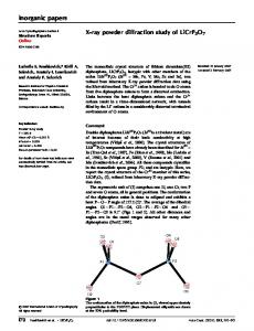
where d is the distance between the planes, λ is the wavelength of the X-rays and θ is the angle of diffraction. By changing the orientation of the crystal sample, it is possible to expose another diffraction plane of the crystal and hence to reconstruct finally the three-dimensional structure of the sample. Characteristic diffraction patterns comprise discrete spots (Laue spots) of high intensities created by coherent interference of X-rays diffracted on parallel planes. The only condition is that the distance between two planes has to be greater than half of the X-ray wavelength (for d < λ/2 ⇒ sinθ > 1). An example of X-ray diffraction on a protein sample is shown in figure 1.14.

1.2.2.1

Powder diffraction

By using a polycrystalline powder instead of a single crystal, the randomly organized small crystals of the powder provide every possible atomic plane orientation that fulfil the Bragg’s condition. Each group of reflecting planes diffracts X-rays with the same angle, thus giving rise to a number of diffraction cones (Debye cones) as depicted in figure 1.15a. The resulting pattern is composed of diffraction rings

18


Figure 1.14: Laue spots as a result of X-ray diffraction on a protein sample (from [3]).

centred on the beam axis, each of them being composed of indistinguishable Laue spots that form a continuous line (figure 1.15b).

a)

b) Figure 1.15: (a) View of the Debye cone resulting from X-ray diffraction diffraction on a polycrystalline sample and (b) the resulting diffraction pattern (from [49],[99]).

Chapter 2 Semiconductor pixel detectors Position sensitive detector provide an information on the impact position of a particle. They have been intensively developed in the last decades and can be found presently in many applications related to radiation detection. Pixel detectors can offer high spatial resolution and thus are widely used in medical application, crystallography and tracking vertex detectors in High Energy Physics (HEP). In the semiconductor radiation detectors, signal arises from a charge generated by an incoming particle. The collected charge is further processed by the frond-end electronics. The read-out electronics may be either a separated chip connected to the detector (strip or pixel hybrid detector), or it may be integrated on the same substrate as the detector (e.g. monolithic pixel detectors or charge coupled devices).

2.1

Principle of operation

2.1.1

Semiconductors physics

To understand the, principle of semiconductor detectors a primary knowledge on semiconductor physics is required. In this section, selected aspects necessary to comprehend operation of semiconductor pixel detectors will be discussed.

19

20

CHAPTER 2. SEMICONDUCTOR PIXEL DETECTORS

2.1.1.1

Energy band model

The electrical parameters of solid materials can be described using the energy band model. The band theory assumes that in a condensed materials, such as crystals, electrons can occupy energy levels grouped in bands. In a solid material composed of N closely spaced atoms, electrons of an adjacent atom are reciprocally influenced. The discrete energy levels of each individual atom do not remain, but become grouped in bands (formed by many closely spaced energy levels of single atoms). Allowed energy bands are separated by a forbidden band, which consists

Figure 2.1: Energy levels of silicon atoms as a function of lattice spacing (from [64]).

in energy levels that are not available for electrons. Energy levels as a function of lattice spacing for silicon are shown in figure 2.1. At large distances, atoms have the same energy levels. As lattice spacing decreases, these levels start to form energy bands. Within a given material, two distinct energy bands are important to determine its electrical properties. The highest completely filled energy band at a temperature of 0 K is called the valence band. The band placed above, partially filled or empty, is called the conduction band. In order to bring the material into a conduction state, electrons needs to move by changing their quantum state. Therefore this movement is possible only towards the unfilled conduction band. In figure 2.2, three types of materials depending on their electrical properties are presented. In the case of a wide forbidden gap, electrons from the valence band cannot acquire enough energy to jump to the conduction band in order to contribute to conduction. Such material is an insulator. In the case of a conductor, the valence and conduction bands overlaps, or the conduction band is partially filled. In both cases, many vacant states are available for electrons. The third group

2.1. PRINCIPLE OF OPERATION

21

Figure 2.2: Different types of materials depending on the energy band structure (Eg - forbidden gap).

of materials in figure 2.2, the semiconductors, have a relatively small forbidden gap with an empty conductive band and a filled valence band at low temperature. However, thermal excitation at room temperature is sufficient to transfer a few electrons to the conduction band, thus leading to a weak conductivity. Two types of semiconductors depending on their band gap structure are recognized. These are the direct-band and the indirect-band semiconductors. When an electron, due to excitation, is promoted from the valence to the conduction band, one needs to care about momentum conservation. In the case of a direct-band semiconductor,

Figure 2.3: Direct-band and indirect-band types of semiconductors.

the highest state of the valence band and the lowest state of the conduction band have the same momentum (figure 2.3). For indirect-band semiconductors, besides energy, an electron needs to change its momentum in order to pass trough the band gap. In most of the cases, this is done with phonon assistance.

22 2.1.1.2

CHAPTER 2. SEMICONDUCTOR PIXEL DETECTORS Intrinsic and extrinsic semiconductors

Intrinsic semiconductors contain a negligible concentration of impurities compared to thermally generated electrons and holes. Each electron, thermally elevated from the valence band to the conduction band, leaves a hole behind it. In an intrinsic semiconductor, the numbers of generated holes and electrons are approximately the same. The density of free electrons, n, and of holes, p is given by n = NC e − p = NV e −

EC −EF kT

(2.1)

EF −EV kT

(2.2)

where NC , NV are the effective densities of energy states in the conduction and valence bands, EC and EV are the energy levels of the conduction and valence bands, k is the Boltzmann constant and T is the absolute temperature. EF is the Fermi level, which corresponds to the energy at which the probability of occupation for an electronic state is one half. The product of electron and hole concentrations is given by np = ni 2 (2.3) where ni is the intrinsic carrier density. The relation 2.3 is called the mass action law. For intrinsic semiconductors, the Fermi level is derived from the assumption that the numbers of electrons and holes are equal n = p = ni and expressed by 3kT EC + EV + ln Ei = 2 4

mp mn

(2.4)

where mp and mn are the effective masses of holes and electrons. The intrinsic Fermi level Ei is located in the middle of the forbidden gap, since the deviation due to the second term of the sum is only of the order of 0.01 eV . Intrinsic semiconductors are rather weak conductors, because this property depends strongly on the purity of the material and on its temperature. The improvement of the conductivity of a semiconductor is obtained by doping, which consists in adding small amounts of impurities to the material. Impurities replace crystal lattice atoms, thus introducing new energy levels in the forbidden gap of the material. Doped semiconductors are called extrinsic. The doping material is chosen in such a way that it has a different number of valence electrons than a semiconductor atom, thus adding new electrons or holes (figure 2.4). Dopants that bring extra electrons are called donors and those that bring extra holes acceptors. In case of donors, the introduced energy level is very close to the conduction

23


Figure 2.4: Crystal lattice bond structure (top) and energy band model (bottom) of (a) intrinsic, (b) n-type and (c) p-type semiconductors.

band. At room temperature, all donor states are ionized and all donor electrons are transported to the conduction band. Hence, the concentration of electrons, n, is equal to the concentration of donor atoms, ND . Therefore, donor doped materials are called n-type semiconductors. Similar considerations can be made, for acceptor type dopants. In that case, an additional energy level is placed close to the valence band. In order to create a valence band with crystal atoms, acceptors will trap an electron from the valence band, thus leaving a hole behind them. The concentration of created holes, p, is equal to the concentration of acceptor atoms, NA . Acceptor doped materials are called p-type semiconductors. In both cases, the intrinsic Fermi level is shifted towards the conduction or the valence bands for donors or acceptors, respectively. New energy levels are expressed by

EF

 ND   , donor dopant Ei + kT ln n i =  NA  Ei − kT ln , acceptor dopant ni

(2.5)

According to the mass action law (eq. 2.3), the increase of majority carriers (electrons in n-type materials and holes in p-type materials) is accompanied with a decrease of minority carriers.

24


Figure 2.5: Change of the silicon band gap depending on the material used as a donor or an acceptor.

As an example, the band gap modulation of silicon with different types of dopant materials [64, 78] is shown in figure 2.5. Silicon have four valence electrons, hence acceptor materials from the boron group with three valence electrons are used, and materials from the nitrogen group with five valence electrons are used as a donors.

2.1.1.3

Charge generation and recombination

There are two main mechanisms of charge generation in a semiconductor: thermal excitation and charge particle interaction. The energy needed to promote an electron from the valence to the conduction band strongly depends on the type of semiconductor and on its energy gap (table 2.1). Thermal generation is often a parasitic process that leads to a rise of leakage current in radiation detectors,

Atomic Number Z Density [g/cm3 ] Energy gap [eV ] Energy/e-h pair [eV ] Intrinsic resistivity [Ωcm] Electron mobility [cm2 /(V s)] Hole mobility [cm2 /(V s)] Electron lifetime [s] Hole lifetime [s]

Si 14 2.33 1.12 3.62 320000 1450 450 10−4 10−4

CdTe 48 (Cd) 52 (T e) 6.2 1.4 4.4 ≈ 109 1000 80 10−6 10−6

Ge 32 5.32 0.66 2.9 50 3900 1900 10−4 10−4

GaAs 31 (Ga) 33 (As) 5.32 1.424 4.2 3.3 × 108 8500 400 10−8 10−8

Table 2.1: Properties of different semiconductors at a temperature of 300 K (from [64],[83]).


25

and hence to signal degradation. Thus, for several materials with a small energy gap, such as germanium (Ge), it is necessary to operate them at low temperatures in order to decrease the influence of leakage current. In radiation detectors, the signal comes from the ionization by the impinging particle. Depending on the type of radiation, the shape of ionization paths are different, involving sometimes secondary processes. In case of X-rays, many electron-hole pairs are generated in a small spatial region around the interaction point. The number of electron-hole pairs, N , may be estimated from the energy needed to generate one electron-hole pair given by N = Exray /Ee−h . The thermal generation rate is independent from the concentration of donors and acceptors and is given by Gth = ni /τg , where τg is the generation lifetime. Under a thermal equilibrium, a continuous balance between generation and recombination of electron-hole pairs occurs, Gth = Rth , according to the mass action law (equation 2.3). Depending on the type of semiconductor, the thermal recombination rate is limited by the concentration of minority charge carriers, i.e. Rth = p/τrn for n-type semiconductors and Rth = n/τrp for p-type semiconductors. Factors τrn and τrp are recombination lifetimes in n- and p-type semiconductors. The excess of carriers created by radiation or injection disturbs this equilibrium. When the external stimulus is stopped, an equilibrium state will be eventually reached by the process of recombination regulated by the lifetime of excess minority carriers τr . On the other hand, if all charge carriers are removed from the semiconductor (e.g. by applying an external voltage), thermal generation will be the dominating process while the recombination rate will be very low. The equilibrium state will be reached again with a time constant determined by the generation lifetime τg . The above explanation is valid for direct semiconductors. In case of indirect materials, processes of generation and recombination are significantly different. The probability of direct band-to-band recombination in indirect semiconductors

Figure 2.6: Mechanisms of generation and recombination trough energy states in the forbidden gap.

26


is very small due to different crystal momentum between electrons of the conduction band and holes of the valence band (see figure 2.3). Recombination occurs as a step process that involves emission/capture of electrons/holes into intermediate energy states in the forbidden gap called generation/recombination centers. Generation/recombination centers consist of semiconductor defects or impurities. Mechanism of charge carrier trapping and emission are shown in figure 2.6.

2.1.1.4

Charge carriers transport

Motion of free charge carriers occurs through scattering on crystal lattices and impurities. This results in random direction movements. Hence, there are no net displacements at thermal equilibrium. In that case, we are dealing with a thermal motion defined by the mean free time between collisions τc , and by the velocity acquired between collisions vth . The characteristic length of thermal motion is lth = vth τc . Typically, at room temperature (300 K), τc ≈ 10−13 − 10−12 s, vth ≈ 107 cm/s and lth ≈ 100 ˚ A. An electric field, E, applied to the semiconductor causes acceleration of the carriers in the direction defined by the electric field. The motion of charge carriers caused by the electric field is called drift current. During a mean free time, τc , carriers gain a velocity defined by

vdrif t

 qE   τc = −µn E, for electrons − mn = qE   for holes  τc = µp E, mp

(2.6)

where µn and µp are the mobility of electrons and holes. An increase of the electric field induces a saturation of the carriers velocity. These parameters strongly depend on the temperature and doping concentration. Carriers mobility for different materials are collected in table 2.1. The drift current density is given as follows

Jdrif t =

 −qnv qpv

drif t,n

drif t,p

= −qnµn E, for electrons

= qpµp E,

(2.7)

for holes

The diffusion current arises in the presence of an inhomogeneous gradient distribution of free charge carriers. The diffusion current has a direction opposite to the concentration gradient, since the carriers move predominantly from the region of higher concentration towards the region of lower concentration. The diffusion


27

currents for the two types of carriers are given by

Jdif f

 qD ∇n, for electrons n = −qD ∇p, for holes p

(2.8)

where Dn and Dp are the diffusion coefficients for electrons and holes. Diffusion coefficient and mobility are related trough the Einstein relationship Dp kT Dn = = µn µp q

(2.9)

where the fraction kT /q is known as the thermal voltage and is equal to 25 mV at 300 K . The total current for one type of carriers is the sum of the diffusion and drift currents: Jn = Jdrif t,n + Jdif f,n = qnµn E + qDn ∇n (2.10) Jp = Jdrif t,p + Jdif f,p = qpµp E − qDp ∇p and the total current in the semiconductor is given by Jtotal = Jn + Jp

2.1.2

(2.11)

Charge collection

The charge in a semiconductor detector originates from direct ionization caused by a traversing particle. The electron-hole pairs created during this process are separated by the presence of an electric field across the active volume. In order to limit the leakage current in the device, different sensor structures are implemented depending on the material. For low band gap materials, like silicon, a junction is required in order to limit leakage current at room temperature. A commonly used structure for this type of semiconductor is the reversed biased p-n junction with a depleted region acting as an active volume for signal detection. For other materials with inherent high resistivities, e.g. diamond, a simple ohmic contact is sufficient. The p-n junction is formed when two adjacent regions of semiconductors are differently doped forming n- and p-type materials in one piece of material. Majority carriers from one side diffuse towards the other side (i.e. holes from the p-side towards the n-side and electrons from the n-side towards the p-side). Diffused charge carriers combine with dopant ions (i.e. extra electrons with acceptor holes

28


Figure 2.7: Electric characteristic functions of a typical abrupt p-n junction.

and extra holes with dopant electrons), which results in a space charge across the junction (positive in the n-side and negative in the p-side). These space charge prevent electron-hole pairs from recombination. In spite, they drift along the field lines. As a result, the region around the junction becomes free of mobile carriers and is called the depleted region. The potential difference across the depletion zone is called the built-in potential or the junction potential. The built-in potential, Vbi , is equal to the difference of the Fermi potential levels for p- and n-type materials (equation 2.5) and is given by kT ln Vbi = q

ND NA ni 2

(2.12)

At thermal equilibrium, the total negative charge in the n-type side is equal (in

29


absolute value) to the total positive charge in the p-type side of the depletion region, NA Wp = ND Wn , thus conserving the electrical neutrality of the device. In figure 2.7, the characteristic functions of an abrupt p-n junction are plotted. The width of the depleted region1 at thermal equilibrium is given by W =

s

2ǫs ǫ0 NA + ND Vbi q N A ND

(2.13)

In a typical detector diode, one side of the junction has a doping concentration a few orders of magnitude higher than the other, usually NA ≫ ND . Therefore, the depletion region extends mainly into one side of the junction. The width of the depleted region can be now expressed by W =

r

2ǫs ǫ0 1 Vbi q ND

(2.14)

The width of the depletion region can also be increased by applying an external voltage with the same polarity as the built-in potential. It increases proportionally to the square root of the applied voltage. The above equations (2.13 and 2.14) can be used to calculate the external voltage required to deplete completely a semiconductor of given thickness and doping concentrations. A metal-semiconductor contact is created when a semiconductor is joined together with a metal layer. Its structure can be characterized by using the energy band model as it was done for p-n junctions. In order to induce the diffusion of the electron from the semiconductor to the metal, the Fermi energy level of the metal and the semiconductor has to be lined up, so that a voltage across the junction is created, which is equal to the difference between the potential functions2 of the materials (2.15) Vbi = Φmet − Φsem The region around the junction on the semiconductor side becomes depleted from the electrons building up a positive space charge in the vicinity of the junction. In order to establish an equilibrium state, positive charges are compensated by a surface charge at the metal side. The height of the created barrier, called the 2

Obtained by solving the Poisson’s equation for the electric potential ( ddxV2 = ǫρs ǫs0 , where ǫs and ǫ0 are the relative dielectric constant for the semiconductor and the permittivity of vacuum), with the assumption of an abrupt change of dopant concentrations 2 Φ is the energy needed to move an electron from a solid (Fermi level) to the vacuum state. In order to obtain a rectyfing metal-semiconductor contact, the condition Φmet > Φsem has to be fulfilled 1

30


Schottky barrier, is given by: qΦBn = q(Φmet − χ)

(2.16)

where qχ is the electron affinity3 of the semiconductor. The width of the depletion region can be modulated by applying an external potential and is expressed with the same equation as for p-n junctions (eq. 2.14). In order to estimate the time needed to collect the charge created by an impinging particle, a parallel plate detector with a reversely biased silicon p-n junction will be considered (figure 2.8). In a partially depleted detector (Vbias ≤ Vdepl ), the

Figure 2.8: Charge collection with a partially depleted p-n junction.

electric field inside the bulk is expressed as a function of the depth x    2(Vbias + Vbi ) 1 − x , for x ≤ Wd Wd Wd E(x) =  0, for x > Wd

(2.17)

The time needed for charge carriers created at a given point x0 to reach the point x is given by W −x ǫSi (2.18) t(x) = τc ln , τc = W − x0 µqND where τc is the collection time constant, which is independent of the applied voltage, but relates to the doping concentration and carriers mobility. Therefore, the 3

The affinity is the energy needed to move an electron from the bottom of the conduction band to the vacuum state.

31

2.1. PRINCIPLE OF OPERATION time required for carriers to reach the detector electrodes is expressed by

W t = τc ln W − x0

(2.19)

However, when the depletion region does not extend over the full width of the detector, the velocity of the electrons which are drifting towards the low field region will drop to zero around the boundary of the depletion zone. Most of the charges will be collected through diffusion. Some others may recombine in the non depleted region. Therefore, the charge collection time for a partially depleted detector is mainly determined by the diffusion across the non depleted region. Although, it should be said that the charge carriers generated in the non depleted region may not contribute to the total signal. In case they cannot reach the depletion region, they are lost due to recombination processes. The charge collection time is reduced significantly when the detector is operating with a bias voltage exceeding the depletion voltage (Vbias > Vdepl ). In that case, a uniform electric field is added to the electric field distribution (eq. 2.17) 2(Vdepl + Vbi ) x Vbias − Vdepl − Vbi 1− + W W W x + E1 E(x) = E0 1 − W E(x) =

(2.20)

The time needed for charge carriers created at a given point x0 to reach the point x is then given by  x  + E − E E 0 1 0 W W t(x) = (2.21) ln x0 µE0 E0 + E1 − E0 W Hence the individual collection times for holes and electrons traversing the whole detector thickness are given by W E0 ln 1 + tc,p = µp E 0 E1 W E0 ln 1 + tc,n = µn E 0 E1

(2.22)

For example, a silicon detector of 300 µm thickness and 10 kΩ typical resistivity biased with 60 V have collection times of ∼ 10 ns and ∼ 35 ns for electrons and holes, respectively.

32

2.1.3


Signal formation

The signal current is generated on the collecting electrodes by the movement of the generated charges in the active volume of the detector. The electric charge induced on the given electrode can be calculated using the Ramo’s theorem [76], which states that the amount of electric charge generated on the electrode is determined by the position of the drifting charges and the weighting potential, φw (x), of the electrode at this position. For a charge q drifting from the point x1 to the point x2 , the electric charge induced on the electrode is given by Q = q [φw (x2 ) − φw (x1 )]

(2.23)

The instantaneous current induced on the collecting electrode due to the charge motion is expressed by i = Ew qv (2.24) where v is the instantaneous velocity of the electron and Ew is the weighting field of the given electrode. This is obtained by applying an unit potential to the electrode under consideration and by grounding all the others. The distribution of signal weighting potential depends on the geometry of the detector electrodes and is different than the electric field distribution (except for detectors with only two electrodes or pad detectors with electrodes significantly bigger than the thickness of the detector). In the case of a pixel detector, the weighting potential is highly concentrated in the region of the signal electrode. Thus, most of the current is generated while the moving charges get close to or directly on the signal electrode. Otherwise, if the charges will not end on the measurement electrode, the signal current induced on this electrode will be canceled. The induced electric charge, which is due to the motion of both types of charge carriers, electrons and holes, towards the opposite electrodes, has a net effect on the positive current of the negative electrode and on the negative current of the positive electrode. When a charge is not collected on the measurement electrode, it then induces a current on this electrode that will change the sign of the measured current and sets its integral to zero (figure 2.9).


33

Figure 2.9: Plot of the weighting field in a segmented detector (from [75]).

2.1.4

Noise in semiconductor detectors

Noise optimization in a semiconductor detector is required in order to improve SNR (Signal-to-Noise Ratio) and consequently energy resolution of the detector. Detector noise and electronics noise cannot easily be treated separately. However, the ultimate achievable noise performance is limited by two physical phenomenons in the sensor itself, independently of the following electronics. The first one is the variance of the number of charges produced by an incoming particle. As already stated, this number of charges is related to the impinging particle energy by E N= (2.25) Eeh If this energy transfer follows a Poisson law, the variance of N would simply be V (N ) = N . Hopefully, this is not true and V (N ) = F N , where F is the Fano factor, F = 0.2 in case of semiconductors. This means that, even with a perfect chain (detector and electronics), an incoming energy E will produce a gaussian shaped peak of variance E σ2 = F N = F (2.26) Eeh As an example, the standard deviation of Gaussian peak produced by an incoming energy of 25 keV will be of ∼ 37 e− , corresponding to a FWHM4 of 370 eV . 4

Full Width at Half Maximum

34


The second physical phenomenon limiting noise performance is related to the variance of the number of charges created by thermal generation in the sensor. This generation follows also a Poisson law and its variance is V (Nth ) = Nth . In the case of a reverse bias diode, this is usually expressed in terms of a reverse current, Ir . Suppose that we integrate the signal from the sensor during a time period τ , we will then integrate also the reverse current during the same time period and therefore, the integrated charge due to this current will be Ir τ . The variance of this charge is also Ir τ and, as before, this leads to a Gauss distribution of σ 2 = Ir τ . This means that for slow systems (large τ ), the reverse current is an crucial issue.

2.2

Semiconductor pixel detectors

In this section, selected architectures of pixel detectors for X-ray imaging in life sciences and for experiments in synchrotron radiation experiments will be discussed.

2.2.1

Charge Coupled Devices (CCD)

The Charge Coupled Device (CCD) is a matrix of Metal-Oxide-Semiconductor capacitors (MOS), each of them representing one pixel. The working principle of CCD is the displacement of charges collected in potential wells within the space charge region. A cross section of the device is shown in figure 2.10. The potential pockets where the charges generated by the radiation are collected, are created by operating the device in over-depletion mode and applying different potentials to adjacent gates of the capacitors. This creates a potential barrier under the neighboring gates that confines the charges collected in the region under the gate with the highest potential. Since all capacitors in one column have a common gate, the charges in one pixel are isolated against spreading in the direction of the gate by implanting channel stoppers (p strips implantations). In order to move charges in the shift-register manner, every third gate is kept on the same potentials Φ1 , Φ2 and Φ3 . Appropriate clocking of these voltages will cause the displacement of the charges along the row in one direction towards the readout anode as depicted in figure 2.10. A big advantage of CCD devices is the very high granularity and the possibility to build large scale devices. In addition they do not have any dead zones. However, the readout of this type of the detector is a relatively slow process, which becomes a real issue in the case of large surface detectors. Moreover, because charges need

2.2. SEMICONDUCTOR PIXEL DETECTORS

35

Figure 2.10: Cross section of a three phase CCD with a charge transfer diagram. Sequential change of the voltages applied to gates Φ1 , Φ2 and Φ3 cause charge transfer from one cell to the other towards the readout anode located at the and of the row.

to be moved through a large number of elements, the transfer efficiency is a very important parameter of the CCD device. Another aspect is the weak radiation hardness, which affects the charge carriers lifetime and the charge trapping occurrences, and consequently results in a degradation of the charge transfer efficiency. Different architectures of CCDs were studied in order to improve key parameters and to make them practical devices in various fields of use ( [64],[102]). The buried-channel or two phase CCD was designed in order to improve the charge transfer efficiency and speed. Another example are pnCCDs with fully depleted silicon substrate and with enhanced sensitivity and fast readout for X-ray detection applications in astronomy, crystallography or medical imaging.

2.2.2

Monolithic pixel sensor

The architecture of a monolithic pixel detector assumes that the sensor is integrated in the same substrate with its readout electronics. Different approaches to developing these types of devices were studied and undertaken. They are mainly

36


driven by the needs for vertex tracking detectors for future colliders (e.g. International Linear Collider (ILC)). The most important (and most challenging) requirements for these detectors are the small size of pixels, the high rate data acquisition and the low material budget. In this section, Monolithic Active Pixel Sensors (MAPS) built in standard CMOS technology will be presented in more details. Indeed, these are the most advanced developments and are currently the only devices of this type that have the potential to build large area detectors. It should be noted, however, that there is ongoing research and development on different concepts of (semi-)monolithic pixel sensors (e.g. DEPFET5 detectors [2]), although these cannot offer yet a small pixel pitch or large surface detector.

2.2.2.1

Monolithic Active Pixel Sensor (MAPS)

A cross-section of MAPS built in standard CMOS technology is shown in figure 2.11a.

a)

b) Figure 2.11: Monolithic Active Pixel Sensor built in standard CMOS technology: (a) cross section and principle of operation, (b) basic pixel architecture based on three N-MOS transistors and a collecting diode (3T pixel).

The availability of slightly doped epitaxial silicon layer in CMOS process is essential for MAPS design. It is grown on top of a low resistivity silicon bulk. The active element in this design is a n-well/p-epi diode. Only the region under the n-well is depleted. Charges liberated by a traversing particle are kept in this thin epitaxial layer (usual of a few to 15 µm thickness) by potentials of p-wells located at the border of the pixel and reach the region of the collection diode by thermal diffusion. Charge carriers generated in the substrate can contribute to the total 5

Depleted Field Effect Transistor


37

signal charge only if they were generated at the border of the epitaxial layer. A big difference of doping levels between the substrate and the epitaxial layer results in a decrease of charge lifetime, since charges recombine in the substrate before they can be collected. The charge signal is usually very small. Therefore, low noise electronics is a critical issue in this development. A typical three transistors based pixel architecture (reset (M1), source follower (M2) and row select (M3)) is presented in figure 2.11b. One of the advantages of this design is its high granularity (a pixel pitch < 15 µm is possible), due to a simple architecture of the single pixel and to the use of a commercial CMOS process. In addition to this, through thinning of the p-substrate and back-illumination, a 100% fill factor can be achieved. The main disadvantage of MAPS devices in standard CMOS technology is that the electronics read-out must consist only of NMOS transistors. In a twin-tube standard process, a P-MOS transistor has to be embedded in a n-well in order to get the positive bias. Since the n-well is used as a collecting diode, any other implantation of n-well would decrease the collected charge signal. Different attempts have been undertaken to overcome this limitation. One of them is to use a non-standard Silicon on Insulator (SOI) technology, with a buried oxide layer (SiO2 ) used to isolate the fully depleted substrate from the electronically active

a)

b) Figure 2.12: Different MAPS designs that allow use of both N- and P-MOS transistors in non-standard technologies: (a) in Silicon on Insulator (SOI) technology, (b) using INMAPS (Isolated N-well) process what allows deep p-well implants.

38


silicon on top of the insulator [57]. The charge collection is done by vias connecting the readout electronics with the substrate through the oxide. A schematic view of the device is shown in figure 2.12. Another approach is to use deep p-well implantation, which provides effective isolation (INMAPS process [5],[19]) of the n-well with P-MOS transistors (figure 2.12(b)).

2.2.3

Hybrid pixel detector

In the hybrid pixel detector architecture, the sensor and the electronics chips are fabricated on different substrates, thus ending with two separate chips. The development of this type of detector was initiated for vertex detectors for HEP experiments (e.g. LHC6 experiments ATLAS7 , ALICE8 , CMS9 and LHCb10 at CERN). The needs for these experiments was to achieve high spatial resolution, high timing precision (event time stamps) and high radiation tolerance. Hybrid pixel detectors have successfully fulfilled all these requirements and large surface detectors (e.g. ∼ 1.7 m2 for ATLAS [105] and ∼ 1 m2 for CMS [106]) were successfully built, thus empowering the reliability of the technology.

a)

b) Figure 2.13: Hybrid pixel detector (a) cross-section and (b) SnPb bumps used for the sensor and electronics chip interconnection.

The separation between readout electronics and sensor electronics allows to optimize the sensor and readout parts independently. The two elements of the detector 6

Large Hadron Collider A large Toroidal LHC ApparatuS 8 A Large Ion Collider Experiment 9 Compact Muon Solenoid 10 Large Hadron Collider beauty 7


39

are connected together in the final stage of the production via the flip-chip technology (figure 2.13(b)). A cross-section through a hybrid pixel detector is shown in figure 2.13(a). A sensor of n-type high resistivity silicon with p+ pixel implants is most often used, but it is also possible to use different materials with higher atomic number and higher efficiencies (e.g. CdTe, CdZnTe or GaAs). The readout electronics chip is designed in a standard, commercial CMOS process with a high density of transistors. Since the sensor part is completely separated from the readout part, this type of pixel does not suffer from any limitation and allows for various signal processing schemes that can be tuned for every given application. The front-end part is always built with a charge amplifier followed by a comparator. The basic pixel architecture of a hybrid pixel detector for X-ray detection is made of three main blocks: charge detection, signal selection and local hit memory. The charge detection block converts the charges generated in the sensor, which gives rise to the voltage (current) signal that is afterwards compared with a detection threshold. The comparison results are then stored in a local memory (counter). The ability to detect and count individual radiation quanta, and thus to image selected energies extends the use of hybrid pixel detectors to different fields of imaging like medical imaging and synchrotron radiation experiments. However, integration of the entire amplifying, thresholding and signal processing electronics in each one of the pixels limits the granularity of the detector and hence spatial resolution. Additionally, the high complexity and the many production steps (chip and sensor production, bump-bonding and flip-chip) result in a lower production yield that makes these detectors quite expensive devices. The hybrid pixel detectors have several advantages over the other detector architectures. The most important one is the significant suppression of the electronic noise, which must result in improved SNR and contrast in the image. Moreover, the adjustable threshold makes it possible to select the energy range of the photons. Especially, in the field of biomedical imaging, this feature can be used to optimize the detection of contrast agents while reducing the total exposure dose. In addition to all the foregoing, hybrid pixel detectors show high radiation tolerance and can achieve very fast readout. In this thesis, the XPAD3 hybrid pixel detector will be discussed in details. But before we give a thorough description of the XPAD3 detector developed at CPPM, we will review some of the state-of-the-art hybrid pixel detectors that have already been developed elsewhere.

40


At present, the most mature designs that allow to build large surface detectors for imaging applications are the PILATUS, the MEDIPIX, and of course the XPAD designs. The first two designs are described in the next part of this section, whereas the detailed description of the XPAD detector is given in the next chapter. Last but not least, we also mention hybrid pixel detectors designed for vertex tracking detectors used in High Energy Physics, and a few other interesting specific developments and applications of hybrid pixel detectors.

2.2.3.1

Hybrid pixel detectors in High Energy Physics

As it was stated at the beginning of this chapter, the development of hybrid pixel detectors was initiated by the needs of High Energy Physics. The main requirements for charge particle tracking are very good spatial and timing resolutions, long term operation performance and high radiation tolerance to doses up to 500 kGy [93]. Hybrid pixels met all these requirements and are currently being used in the inner detector for several experiments of the LHC at CERN and of the Tevatron at Fermilab11 close to the interaction point. The application to particle

a)

b) Figure 2.14: (a) Layered view of the ATLAS pixel detector module and (b) picture of a CMS pixel detector module.

tracking imposes a number of requirements for the pixel design such as low power consumption, low noise and low threshold dispersion, zero suppression in every 11

Fermi National Accelerator Laboratory: http://www.fnal.gov/


41

pixel or on-chip hit buffering. Every hit registered in the pixels is assigned to the corresponding collider bunch crossing. The main developments were carried out for the ATLAS and CMS experiments at CERN. The pixel sizes are 50 × 400 µm2 for ATLAS and 100×150 µm2 for CMS. For ATLAS and CMS, a detection module is composed of 16 readout chips bump bonded to a single silicon sensor. The chips are generally wire-bonded to a kapton flexible circuit that is glued atop the sensor (figure 2.14). The module is controlled via a Module Control Chip (the MCC) that is placed on the flexible circuit and is responsible for the front end trigger control and event building.

2.2.3.2 2.2.3.2.1

The PILATUS II and EIGER hybrid pixel detectors PILATUS II

The PILATUS II12 detector is a silicon hybrid pixel detector that was designed for crystallography experiments at the Swiss Light Source (SLS) of the Paul Scherrer Institute (PSI) [45],[103]. The PILATUS II detector is the successor of the PILATUS I [9], [44] detector with improved functionality and corrections for several shortcomings. The PILATUS II readout chip (ROC) was designed in a standard 0.25 µm CMOS process using radiation tolerant layout techniques. The ROC is composed of 5820 pixels organized in a matrix of 60 × 97 pixels with a size of 172 µm × 172 µm. The main properties of the PILATUS II readout chip are presented in table 2.2. The pixel design comprises a charge sensitive preamplifier (CSA), an AC coupled shaper, a comparator and a 20-bit counter. The threshold level of the comparator is adjusted with a global threshold voltage and can be locally trimmed for each pixel with a 6-bit DAC. The digital output of the comparator feeds the 20-bit counter, in which the overall number of detected photons is stored. The architecture of the pixel cell is shown in figure 2.15. Every pixel can be individually selected by addressing it with two signals, ROWSEL and COLSEL. These two registers allows for reading and writing the pixel counter and the 6-bit DAC, as well as for sending a calibration signal (CAL). The ROC can operate in two different modes: the count mode and the readout mode. During the count mode, no pixels are selected and, as long as the external enable signal is logic high, every pixel is counting photons. In the case of the readout mode, 12

Pixel aparatus for the SLS

42


Figure 2.15: The pixel design of the PILATUS II readout chip (from [55]).

each pixel is sequentially selected in order to read its counter value via the digital output signal (DOUT). A single PILATUS II detection module is formed by an array of 8 × 2 ROCs bump bonded to a single silicon sensor with a thickness of 320 µm. The single module contains 94′ 965 pixels in an array of 487 × 195 pixels. In order to avoid dead areas between the chips, the sensor consists of two rows of pixels of size 1.5 times larger than a normal pixel (258 × 172 µm2 ). The counts of these pixels are distributed by the software into three pixels of normal size, thus introducing a virtual pixel. The same logic is applied to the corners of the chips. However, in this case, sensor pixels have a size that is 2.25 times larger than a normal pixel (258 × 258 µm2 ), thus introducing five virtual pixels. In total, this technique adds 1′ 845 virtual pixels to the matrix. Every detection module is connected to its module control board (MCB). The MCB board is equipped with an electronics that provides all the necessary voltages and biasing as well as control signals distributed via an I2 C13 interface. In order to have a fully operational detector system, one module have to be connected to a detector control board (DCB). The system requires a separate power supply and an acquisition computer. The PILATUS II detector has a modular architecture, which means that a large surface detector of any size can be assembled, providing it consists in a multiple of 487 × 195 pixels. The PILATUS II modules were used to build a large hybrid pixel detector, the PILATUS 6M, which is currently in use at several synchrotron beamlines. The PILATUS 6M is built of 5 × 12 modules with 2436 × 2527 = 6′ 155′ 772 pixels. The total active area of this detector is 424 × 435 mm2 . One 13

Inter-Integrated Circuit

PILATUS II

EIGER

Pixel size

Count rate

[µm2 ]

[ph/px/s]

60 × 97 5′ 820

172 × 172

2 × 106

20 bits

256 × 256 65′ 536

75 × 75

16 × 106

MEDIPIX2

256 × 256 65′ 536

55 × 55

106

XPAD3

80 × 120 9′ 600

130 × 130

106

Table 2.2:

Counter depth

Readout time

Energy range

Power (analog.)

Noise (rms)

CMOS technology

µW

Thresh. dispers. (rms) e-

[keV]

e-

µm

2.85 ms

3-30

-

50

125

0.25

12 bits (4, 8, 12 mode)

85 µs 8-bit mode

-

9

20

180

0.25

13 bits

8.5 ms in serial 266 µs in parallel

8

500

105

0.25

5-300

12 bits + OVF

1 ms

5-35

40

50

130

0.25


Num. of pixels

Technical specifications of the PILATUS II, EIGER, MEDIPIX2 and XPAD3 detectors (based on data from [97],[29],[35],[55]).

43

44


module of the PILATUS II detector is shown in figure 2.16 alongside with the PILATUS 6M detector system.

a)

b) Figure 2.16: (a) PILATUS II single detector module and (b) PILATUS 6M detector system.

A spin-off company of PSI, named DECTRIS Ltd. was founded in 200614 to commercialize hybrid pixel detector systems based on the PILATUS II chip. Comparison of the main parameters between some PILATUS detectors and the XPAD3 detector is shown in table 2.3.

2.2.3.2.2

EIGER

The EIGER15 detector is another hybrid pixel detector designed at PSI for the SLS. As a successor of the PILATUS II detector, its design has several improvements, including in particular a smaller pixel pitch and faster readout time. Similarly to its ancestor, the EIGER readout chip was designed in 0.25 µm technology using radiation tolerant layout techniques. The pixel size was scaled down to 75 µm × 75 µm and a single chip contains 65′ 536 pixels organized in a matrix of 256 × 256 pixels. The specification of the EIGER chip is presented in table 2.2. The threshold level of the comparator is globally set for all pixels and trimmed individually for each pixel with a 6-bit DAC. The output of the comparator feeds a double buffered 12-bit counter with overflow management. The counter can operate in three modes using 4, 8 or 12 bits. A single detector module is formed with eight chips (organized 14 15

Dectris Ltd.: http://www.dectris.ch Extreme high frame rate detector

45


100K

PILATUS 300K

1M

83.8 × 33.5 mm2

83.8 × 106.5 mm2

169 × 179 mm2

75 × 120 mm2

Number of pixels

487 × 195 94′ 965

487 × 619 301′ 453

981 × 1043 1′ 023′ 183

560 × 960 537′ 600

Number of modules

1

3 (1 × 3)

10 (2 × 5)

8 (1 × 8)

none (one module)

5.5%

8.4%

none (tiling)

Framerate

300 Hz

200 Hz

30 Hz

240 Hz

Weight

∼ 4 kg

∼ 10 kg

∼ 25 kg

∼ 15 kg

Area

Intermodule gap

XPAD3

Table 2.3: Comparision of the main parameters between some detectors of the PILATUS family and the XPAD3 detector (from [97],[16]).

in two rows of four chips) bump bonded to the sensor material. Each half-module (one row of four chips) is connected to a back-end board equipped with memory and processing electronics. The EIGER chip is currently undergoeing tests at PSI to verify its design and functionality.

2.2.3.3

The MEDIPIX family of hybrid pixel detectors

The MEDIPIX family of hybrid pixel detectors includes the MEDIPIX1, MEDIPIX2, TimePix and MEDIPIX3 chips. These chips are being developed within a collaboration between many universities and research institutes, mainly from Europe. In this section, the MEDIPIX2, TimePix and MEDIPIX3 chips are introduced in more details.

2.2.3.3.1

MEDIPIX2

The MEDIPIX2 chip is designed in 0.25 µm technology. It consists of a matrix of 256 x 256 pixels, each of them having a size of 55×55 µm2 . Technical specifications of the MEDIPIX2 chip are shown in table 2.2. The main components in the pixel design are the charge preamplifier with DC leakage current compensation, the double discrimination logic and the 13-bit counter.

46


The pixel cell is shown in figure 2.17. Changing of the bias conditions of the

Figure 2.17: Pixel design of the MEDIPIX2 readout chip (from [63]).

preamplifier makes the chip sensitive for holes and electrons. The two comparators allow for energy windowing. Upper and lower energy settings are performed thanks three configuration bits per discriminator. Each pixel has two modes of operation that are selected with the input signal shutter : the acquisition mode and the shift mode. In the acquisition mode, the output of the double discrimination logic acts as the clock of the counter. In case of the shift mode, data are shifted from pixel to pixel in order to read out and write in the pixels. The MEDIPIX2 circuit can be read out in a serial mode using high speed LVDS signal or in a parallel mode via 32-bits. The MEDIPIX2 circuit was successfully used to build a detector system with different sensor materials and architectures in order to fulfil requirements of experiments performed at synchrotron radiation sources and for biomedical imaging applications. Apart from silicon that is the classical sensor material used for charged particle detectors, the MEDIPIX2 chip was also hybridized with high-Z materials such as CdTe [17] and GaAs [54]. The circuit was also evaluated as a readout chip for a Time Projection Chamber (TPC) [12] gas detector, as well as for a novel 3D architecture of the sensor material [94]. Another interesting development is a neutron pixel detector based on the MEDIPIX2 chip [47]. In order to detect neutrons in the detector sensor, a dedicated layer of a neutron converter was deposited on the silicon sensor surface. Thermal neutrons are converted in this layer into secondary charged particles, which are detected by the MEDIPIX2 detector. In figure 2.18a, a single MEDIPIX2 chip wire bonded


a)

47

b) Figure 2.18: Pictures of (a) the MEDIPIX2 circuit with 300 µm silicon sensor wire-bonded to the probe card and (b) of a four-chip module (quad) connected (in the figure only one chip is wire bonded without a sensor) to the Gigabyte Ethernet link (from [100]).

to the readout chip developed at CERN is shown. In figure 2.18b, four chips are connected to a high speed readout module that was developed in the framework of the RELAXD16 project [91]. The aim of this project is to build large area detector by tiling several modules like the one presented above. In order to minimize dead areas between the modules, it is planned to remove the wire bonding connection to the supporting PCB and replace it by a via through the MEDIPIX2 chip. The CAD visualisation of the RELAXD detector is shown in figure 2.19a and a cross section of the via interconnection in figure 2.19b.

2.2.3.3.2

TimePix

The TimePix chip [8] is a modified version of the MEDIPIX2 chip that has an extended functionality to determine the time of photon interaction and the total charge of an event. The motivation for the design of the TimePix chip was to evaluate its use for a Time Projection Chamber for High Energy Physics. This extended functionality was implemented at the expense of the high threshold setting. The implemented TimePix synchronization logic allows to synchronize the particle arrival time with a reference clock and to use the pixel counter as a timer. The time-stamp approximation has a tunable time resolution of 100 ns down to 10 ns. The total charge information is obtained from a time-over-threshold method. In that case, the counter is used as an ADC that allows for direct energy measurement in each pixel. 16

High REsolution Large Area X-ray Detector

48


a)

b) Figure 2.19: (a) CAD visualisation of the RELAXD detector and (b) a cross section of the via interconnection between the MEDIPIX2 and a supporting PCB.

2.2.3.3.3

MEDIPIX3

The MEDIPIX3 chip is the successor of the MEDIPIX2 circuit. It was designed in 0.13 µm CMOS process and the chip has the same dimensions as the MEDIPIX2 chip, i.e. 256 × 256 pixels of 55 × 55 µm2 size. The main motivation to design this new chip was to reduce the problem of charge sharing between neighboring pixels. Indeed, this was a significant issue for the MEDIPIX2 detector [39],[4]. In the MEDIPIX3 architecture, four adjacent pixels are grouped into a cluster and information about charge deposition in the pixels is shared between the pixels belonging to a cluster. At the corner of each pixel, there is a summing circuit that adds the total charge deposited in sub-group of pixels and an arbitrary logic assigns a hit to the pixel hit with the highest charge. This mode of operation is referred to as the charge summing mode, but the circuit can also be configured in a single pixel mode to operate like a conventional detector system, without this charge reconstruction mechanism. In addition to this, each pixel consists of a preamplifier, a shaper and two threshold discriminators in the analogue front-end electronics. The digital processing circuitry includes a control logic, an arbitration logic for hit allocation, a double 12-bit counter and configuration registers. The low and high threshold levels of the discriminators are set via two 9-bit registers. Each one of the 12-bit pixel counters is registering hits that are associated with one threshold level. The counters can be configured to work with 1, 4 or 12-bits. In addition, both counters can be concatenated and used as a single 24-bit counter. However, only one discrimination level is used in this case. Furthermore, the chip


49

can be configured in such a way that either the size of the readout pixel matches the physical pixel pitch (the fine pitch mode) or is four times greater (110 × 110 µm2 ) by grouping four pixels in a cluster called a super-pixel (the spectroscopic mode). In either case, the charge summing and the single pixel modes are available.

2.2.3.4

Specific developments and applications of hybrid pixel detectors

Besides the above-mentioned hybrid pixel detection systems, several projects were launched in a number of research units worldwide. The most interesting ones are listed below.

2.2.3.4.1

CIX 0.2

The CIX detector [33][34] is a prototype of a simultaneously counting and integrating X-ray chip connected with a sensor material (the CIX chip was hybridized with Si, CdTe and CdZnTe sensors). The device is being developed jointly by the University of Bonn (Germany), the University of Heidelberg (Germany) and the Philips Research Laboratories Aachen (Germany). The CIX matrix is composed of 8×8 pixels with 250×250 µm2 size. The technical characteristisc of the chip are given in table 2.4. The main components of the photon counting part of the pixel design are a charge sensitive amplifier, a fast discriminator and a 16-bit counter. The charge integration circuitry consists again of a charge sensitive amplifier, a comparator and a current integrator. The double mode of photon detection allows for using the detector in a very high photon flux, where discrimination of the photon is no more possible.

2.2.3.4.2

DIXI

The DIXI (DIgital X-ray Imaging) detector [22][32] is a hybrid pixel device developed for dynamic medical X-ray imaging. The detector consists of a sensor bump bonded to the Angie readout chip. The Angie chip was developed in cooperation between the Radiation Science Department of the Uppsala University (Sweden) and the Norwegian ASIC design house Ideas ASA. The readout chip has 992 pixels organized in a matrix of 31 pixels with 270 × 270 µm2 size. The pixel design consists of a preamplifier, a shaper, a discriminator and a two 16-bit counters. A double counter solution allows for acquiring two images from the detector every µs.

50


Number of pixels Pixel size Counting rate Counter depth Features

CIX 0.2

Angie

8 × 8 = 64

31 × 32 = 992

500 × 250 µm2 3 × 106 ph/pixel/s 16 bits photons counting and charge integration in one pixel

270 × 270 µm2 > 106 ph/pixel/s 12 bits double counter

Aladin1 64 × 64 = 4096 (per chip) 64 × 448 = 28672 (per module) 150 × 150 µm2 106 ph/pixel/s 15 bits fast readout of 1 ms

Table 2.4: Technical specification of the CIX 0.2, Angie and Aladin chips.

2.2.3.4.3

LAD1

The LAD1 (Large Area Detector) detector [82][80] was developed for X-ray diffraction by a collaboration between the Imperial College in London (UK), the Glasgow University (UK) and the Rutherford Appleton Laboratory (UK). The detector has a modular structure with a maximum size of 300 × 300 mm2 . Modules are built of seven Aladin readout chips bump bonded to a silicon sensor. The single Aladin chip consists of a 64 × 64 matrix with 150 × 150 µm2 pixels. Each pixel contains a preamplifier, a shaper, a programmable discriminator and 15-bit counter. The maximum count rate per pixel is 106 photons/pixel/s. The readout speed of the module amounts up to 1000 frames/s and the readout speed of the multi-module detector is independent from the size.

Chapter 3 XPAD3 X-ray camera 3.1

Introduction

The XPAD3 detector is the third generation of hybrid pixel detectors developed by the imXgam1 group at CPPM in collaboration with the group of Institut Néel in charge of the D2AM beam line at ESRF2 and the detector group at SOLEIL3 . The design of the first photon counting chip of the XPAD family (XPAD1) was based on a development done at CPPM for the CERN experiment DELPHI4 [25]. The project was carried out in collaboration with the D2AM beamline group at ESRF. The first chip was designed to evaluate the ability of hybrid pixel detectors to be used in experiments for third generation synchrotron radiation sources. The very high brightness of these facilities makes it possible to perform new experiments that require a wide dynamic range and low noise detectors. The XPAD1 prototype demonstrated promising results that led to design a second prototype chip called XPAD2 [6]. A large surface detector (70 × 70 mm2 ) was assembled and successfully used in experiments with synchrotron radiation. In addition to this, ability to image of small animals were investigated [24]. The SOLEIL detector group joined the collaboration for the design of the third prototype chip called XPAD3. The XPAD3 chip was designed in two different versions called XPAD3-S5 1

imaging techniques based on X and gamma radiation European Synchrotron Radiation Facility, address: Polygone Scientifique Louis Néel, 6 rue Jules Horowitz, 38000 Grenoble, France 3 French national Synchrotron facility, address: L’Orme des Merisiers, Saint Aubin - BP 48, 91192 Gif sur Yvette cedex, France 4 DEtector with Lepton, Photon and Hadron Identification 5 S stands for Silicon 2

51

52

CHAPTER 3. XPAD3 X-RAY CAMERA

and the XPAD3-C6 , which are working respectively in holes and electron collection modes. The main difference between both designs is the energy range that is 35 keV for the -S version and 60 keV for the -C version. Conceptually, the XPAD3-C circuit was designed for biomedical applications requiring high efficiency at high photon energies (which in turn means a sensor of high effective atomic number, usually working in e- collection mode) and the XPAD3-S version for synchrotron radiation experiments. The subject-matter of this chapter is the large surface camera built with the XPAD3-S chip.

3.2 3.2.1

XPAD3 photon counting chip Global architecture

The XPAD3 chip was designed in deep sub-micron, radiation hard IBM 0.25 µm technology. Both versions of the chip (XPAD3-S and XPAD3-C) have the same global architecture and differ only in the pixel design. The main parameters of the XPAD3-S and the XPAD3-C chips are presented in table 3.1. XPAD3-S Number of pixels Pixel size Counting rate Chip readout Counter depth Power Input polarity Selectione mode Nonlinearity Electronic noise (rms) Threshold disperssion

XPAD3-C

9600 130 × 130 µm2 ≤ 106 photons/pixel/second < 1 ms 12 bits + overflow < 70 µ W/pixel holes collection electrons collection single threshold double threshold < 10% over 35 keV < 10% over 60 keV < 130 e− ∼ 50 e−

Table 3.1: XPAD3 characteristics.

The topology of the chip is shown in figure 3.1. The main blocks of the circuit are: a matrix of 9600 pixels organised in 80 columns of 120 cells each, readout/write-in shift registers and global configuration registers. In addition, the chip is equipped with a temperature sensor, a test pulse and a bias generator. 6

C stands for Cadmium Telluride, CdTe

3.2. XPAD3 PHOTON COUNTING CHIP

53

Figure 3.1: Global architecture of the XPAD3 chip.

3.2.2

Pixel details

The XPAD3 chip has pixels of 130 × 130 µm2 . The area of the pixel is vertically divided into two sub-cells of 65 × 130 µm2 , one for the analogue front-end electronics and the other one for the digital data processing and the readout. The XPAD3-S pixel chain is presented in figure 3.2. The analogue part of the

54


Figure 3.2: XPAD3-S pixel design.

pixel comprises a charge sensitive amplifier (CSA), an operational transconductance amplifier (OTA) and a current mode comparator7 . The CSA is a low noise, folded cascode preamplifier that transforms the charges received from the detector through the bump pad into a voltage signal. The feedback resistor Rf that resets the 10 fF feedback capacitance is realized as a classical MOS transistor polarised in ohmic zone8 . The output voltage signal is then converted to the proportional current signal by the second stage OTA. This allows for using a current mode comparator with a simple and compact design. The energy threshold value is set globally for all the pixels by a single 8-bit global DAC (section 3.2.4) and the dispersion of the offset is adjusted in every pixel with a 6-bit local DAC (DACL). The discriminator output feeds a 12-bit counter with an overflow bit (OVF). The depth of the counter was determined to permit on-the-fly readout with a photon counting rate up to 106 photons/pixel/s. Thus, reading an overflow bit at a frequency of 250 Hz allows the dynamic of the counter to be increased by the use of external electronics for processing and storage. The counter is enabled via a Counter Enable Gate signal (CEG). The 9-bit local configuration register, among other things, is used to store the DACL value. A detailed description of 7 The XPAD3-C version consists in two separated discriminators for low and high energy thresholds 8 The OTA design in used for the XPAD3-C version of the chip


55

the pixel configuration register in the XPAD3-S9 version is presented in table 3.2. The readout and write-in operations from and into the pixel are performed via a Configuration bit [0] [1] [2] [8:3]

Description Activate counter Activate analogue and digital test Deactivate preamplifier Value of the local DAC

Table 3.2: Description of the XPAD3-S pixel configuration register.

shift-register called lift. This memory is a 12 × 120-bit register per column that allow data to be transferred along the column in both directions. The source of the data for reading the counters or a configuration is selected with a 12-bit multiplexer. Data are copied to the lift and shifted “down” towards the direction to the readout conveyor placed at the bottom part of the circuit (figure 3.1). Beside the 12-bit data lift, there is also 1-bit lift that allows the readout of the overflow or of the output of the discriminator. Data input is done via a 80 × 1-bit “horizontal” shift-register called SR1. In order to increase the transfer rate, data are carried out using a 80 × 4-bit shift-register called SR4. In addition, analogue and digital parts of the pixel are surrounded with guard rings in order to isolate each part from the other as well as adjacent pixels. The analogue part is surrounded with two, p+ and n+ diffusion rings, and the digital part is encircled with one p+ ring. Moreover, in order to enhance the protection of the most sensitive analogue front-end part (the input of the detector) from the influence of the most noisy digital element part that consists in the least significant bit (lsb)10 , the distance between these two parts was maximized (figure 3.1).

3.2.3

Modes of operation

Each of the three parts of the detector (the pixel matrix, the conveyors and the global configuration registers) is designed to perform different actions. The number of inputs in the chip are limited and do not allow to have a dedicated clock and data input for every section of the chip. Thus, a special logic has been designed that is able to decode and execute all operations needed to control the chip with 9

The XPAD3-C version uses two 8-bit registers to set the low and high thresholds. Local dispersion correction is done with 5-bit and 2-bit DACs for low and high energy discriminators, respectively 10 lsb - least significant bit, LSB - least significant byte.

56


Figure 3.3: Programming of the XPAD3 chip modes and actions.

one data input and three clock sources (DataIn, ChipModeClk, ClockModeClk and MasterClk ). Key elements in that design are two configuration registers called ChipMode and ClockMode (figure 3.3). In this section, the available modes of operation depending on the value programmed in these registers are presented.

3.2.3.1

ChipMode register

The ChipMode is a 9-bit register that determines the current mode of operation of the different sections of the chip. In particular, it controls the data flow in the Chip Mode 12 bits or 1 bit mode

Conveyor mode

Pixel data lift mode

OVF or Hit mode

Value Allowed operation SR4 conveyor reg[0]=0 connect SR4 input with pixel lift 1 connect SR4 input with OVF lift reg[1:2]=00 readout of SR4 01 complete reset of SR4 10 write pixels data to SR4 11 write global registers values to SR4 Pixel reg[3:4]=00 read from SR1 01 write to SR4 10 load counter value to pixel lift load configuration register value 11 to pixel lift connect discriminator output with reg[5:6]=00 OVF/Hit lift connect counter OVF bit with 01 OVF/Hit lift 10 write to SR4 11

57


ConfigG lift mode

Global configuration reg[7:8]=00 read from SR1 01 write to SR4 10 not used load global configuration register value to 11 the global configuration lift

Table 3.3: List of XPAD3 modes of operation.

chip. Available modes are listed in table 3.3.

3.2.3.2

ClockMode register

The ClockMode is a 4-bit register that routes one global clock of the circuit (MasterClk ) to the selected block of the XPAD3 chip. Possible destinations of the MasterClk and subsequent triggered actions are listed in table 3.4. Clock Mode 0000 0001 0010 0011 0100 0101 0110 0111 1000 1001 1010 1011 1100 1101 1110 1111

Action Delay General Reset Global Configuration No Test Pulse No Clk DAC TempSensor No Clear DAC TempSensor No SR1/SR4 conveyors Clk SR1 No Clk SR4 No Store Selcol No N/A N/A N/A N/A N/A N/A Pixels Clk DataLift Yes Store Config Yes Store OVF or Hit Yes Counter clear Yes Global Configuration Clk ConfigG Lift Yes Store ConfigG Yes

Allowed operation No No No No No No No N/A N/A N/A Yes Yes Yes Yes Yes Yes

Table 3.4: List of XPAD3 actions triggered by the ClockMode register.

The operation that requires access to many pixels of the matrix may cause problem related to the noise generated by the high activity of the digital electronics. In order to minimize this effect, the global clock signal that synchronizes the readout and write-in processes of the pixels has been distributed in time and space across

58


the matrix. The mechanism called tsunami is based on delaying the MasterClock signal along 80 columns and 120 rows as depicted in figure 3.4. Hence, available actions listed in table 3.4 are divided into those that require the MasterClock signal delayed or not delayed.

Figure 3.4: Distribution of the delayed clock signal.

3.2.4

Global configuration registers

The global configuration registers are placed at the bottom part of the circuit. Every global configuration register has the same design consisting in the digital part of one pixel. Thus, they are called fake pixels or ConfigG. Despite a similar design like for standard pixels, fake pixels have only 9-bit memories. They are organised in a single row that is read and written via the SR4 and SR1 conveyors. Global registers that are available in in the -S version11 of the chip are listed in table 3.5. However, some cells in a row are not only designed to store global configuration data, but have also extended or different functionalities. • column 0: instead of ConfigG, there are cells called IOinterface and Decoder. These are responsible for the reception of the control signal from the IO ports and for the control of the digital part of the chip (registers ChipMode and ClockMode). 11

The XPAD3-C version has three more registers called IthH , Vref and Vadj

59

3.2. XPAD3 PHOTON COUNTING CHIP Register name

Column number

Used bits

CMOS Disable[0]

5

ConfigG[1]

Data TestPulse[7:0] Data Imfp [7:0] Data Iota [7:0] Data Ipre [7:0] Data IthL [7:0]

50 55 56 59 60

ConfigG[8:1] ConfigG[8:1] ConfigG[8:1] ConfigG[8:1] ConfigG[8:1]

Data Itune [7:0]

65

ConfigG[8:1]

Data Ibuffer [7:0]

66

ConfigG[8:1]

Disable MasterClock output[0]

78

ConfigG[1]

Description Deactivation of CMOS output Injection pulse amplitude Rf polarization OTA polarization CSA polarization Low threshold level DAC threshold and compensation Polarization of output buffers Deactivation of MasterClock output

Table 3.5: List of XPAD3-S global configuration registers.

• columns from 1 to 4 and 73 to 76: ConfigTest cells. They can probe some digital functionalities. • columns 39 and 40: instead of ConfigG, these cells are temperature sensor control units. • column 79: Conveyor ComeBack block which is a termination of the SR1 and SR4 conveyors. The ConfigG cells that are not used to store any global configuration can be used by the user as a general purpose memory.

3.2.5

Calibration

One important parameter in the pixel counting chain is the discriminator threshold, particularly with a polychromatic X-ray beam, in order to ensure that each pixel of the matrix is sensitive to the same energy range. As already described above, the global threshold of the matrix is adjusted by setting the IithL parameter. However, the dispersion of the microelectronics process results in a wide pixel threshold distribution all over the matrix. In order to compensate these dispersions, a local 6-bit DAC has been implemented in each pixel. Changing the value of DACL allows to narrow the pixel threshold distribution. Due to the fact that the signal amplitude value is lost after discrimination (figure 3.2), the value of the threshold has to be derived from the digital output of

60


the chip. The method that is used is based on the injection of a given number of pulses of known charge to the analogue front-end electronics. The response of the discriminator is then studied with different threshold settings. As a result, a curve that represents a pixel count rate versus its threshold setting is drawn. This curve has a characteristic S shape and the method of calibration is called S-curve method [30]. An example of an S-curve measured with the XPAD3-S chip is shown in figure 3.5b. The XPAD3 chip is equipped with a charge injector generating a voltage with an amplitude determined by the TestPulse register. An injection pulse is distributed among a subset of pixels and charges the preamplifier of the pixels to permit the adjustment of thresholds. Unfortunately, with the first version of the XPAD3 chip, the injector is penalized by a slow rise time, which modifies the signal shape of the preamplifier. Therefore, the calibration of the detector to a desired energy level cannot be performed by the injection pulse, but requires the presence of an external monochromatic beam of known energy. This problem has been fixed for the second generation of the XPAD3 chip. Another possibility is to calibrate the pixels just above the electronic noise without using an external physical signal, i.e. at the lowest practicable threshold. The generic procedure of calibration is done with the following steps: 1. Setting of all the pixel DACL values to their middle value (DACL=32). 2. Determination of the global threshold value (register IthL ). For this, a loop process is started with the highest possible threshold, i.e. where almost no pixels are counting and the threshold is then gradually lowered. The value of the IihL is then set when half of the pixels are counting. 3. Acquisition of 64 images, each one with a different DACL setting (from 0 to 63)12 . 4. For each pixel, the value of the count rate measured as a function of the DACL value creates a curve with the characteristic S shape. This curve allows for determining the best DACL value for the pixel. When a calibration is performed with an external beam, the DACL value is set by the inflection point of the curve that corresponds to one half of the maximum count rate. For the calibration just above the electronic noise, the DACL value is set to the last silent acquisition with the higher DACL value. 12

By increasing the DACL value, the physical threshold is decreased


a)

b)

c) Figure 3.5: Result of the calibration with 10 keV monochromatic X-ray beam: (a) histogram of the DACL correction, (b) measured S-curve for one pixel and (c) map of the DACL in the matrix.

61

62

CHAPTER 3. XPAD3 X-RAY CAMERA 5. Uploading of the selected DACL values to the pixels.

The result of the calibration at the noise level is shown in figure 3.5. A lateral drift is clearly visible in the map of the DACL values in the chip. This parasitic effect results from the power supply track distribution on the bottom of the matrix [16].

3.2.6

Data transfer

The readout architecture of the XPAD3 is organised in columns that act as shift registers connected to the readout and write-in conveyors. This solution provides a fast and simple readout of the circuit that preserves the reliability of the transfer (in the worst case, only that column will be lost where there is one pixel is broken).

a)

b) Figure 3.6: Architecture of a single cell (a) of the readout conveyor SR4 and (b) of the write-in conveyor SR1.

The readout of pixel and global registers is done via the 4-bit wide and 80-bit length readout conveyor (SR4). The mechanism is based on data shifts from pixel to pixel down to the SR4 register placed at the bottom of the matrix. The following steps need to be taken in order to read the counters or the configuration register: 1. Enable the columns to be read (global operation)

3.3. ARCHITECTURE OF THE XPAD3 CAMERA

63

2. Load the counter/configuration to the data lift (global operation) 3. Load the SR4 register using the 4-bits of the data lift (shift down) 4. Flush the SR4 register Steps 1 and 2 need to be repeated 360 times in order to read the full matrix of pixels (1 column = 120 pixels × 12 bits = 1440 bits). One has to remember that the ChipMode and ClockMode registers have to be correctly programmed before each readout step. The readout of the overflow bit of the counter is done the same way, except data are transferred via the 1-bit OVF/Hit lift. In that case, steps 1 and 2 have to be repeated 30 times for reading the pixel matrix (1 column = 120 pixels × 1 bit). Writing data to the chip is done in a similar way as reading. In that case, data are first loaded to the 1-bit wide and 80-bit length write-in conveyor (SR1), then copied to the data lift and finally shifted towards the pixel. When writing pixel data, the operation needs to be repeated 1440 times before the lift can be copied to the configuration register. It needs to be repeated only 9 times when writing a global configuration.

3.3 3.3.1

Architecture of the XPAD3 camera Overview

The complete XPAD3 camera comprises eight detection modules, the HUB board and a PC equipped with a PCI Express board that is running the data acquisition software (DAQ). The global architecture of the readout electronics of the XPAD3 camera is presented in figure 3.7. Every module is connected to its own processing electronics, which is itself connected to the HUB board via a set of a copper cables. The role of the HUB board is to transfer the data sequentially from the modules to a PCI Express board embedded in a PC via two pairs of optical fibres. When writing from the DAQ, data are decoded and redirected to the correct module. Besides data management, an external gate signal is distributed to the modules via the HUB board in order to be able to perform time resolved experiments. Fast data transfer to the PC are ensured by using Direct Memory Access (DMA) transfer between the PCI Express interface and the PC memory.

64


a)

b) Figure 3.7: (a) Global architecture of the XPAD3 camera readout electronics and (b) picture of the complete camera enclosed in the box.


65

Within this project my contribution consisted in the design and implementation of the readout architecture of the camera. This work consisted in the development of the embedded firmware for every stage of the camera and of a first version of the software library. The firmware development process involved hardware components of the detector equipped with programmable logic (FPGA) such as: the detection modules, the HUB board and the PCI Express board. Communication between the abovementioned components is performed using custom protocols designed within this work. In order to validate the design architecture and to measure the performance of the camera, a preliminary version of the software library was developed. The final device, especially its fast readout, was tested by conducting three experiments designed for this purpose. Moreover, I have participated in several experiments carried out at synchrotron radiation sources. The following sections of this chapter include a description of the camera architecture developed specifically within the framework of this doctoral project.

3.3.2

Detection modules

3.3.2.1

Architecture

Every detection module is composed of seven XPAD3-S circuits placed side by side and bump bonded to a 500 µm thick silicon sensor (figure 3.8a). The size of the module is 75.1 × 15.6 mm2 (560 × 120 pixels). In order to avoid dead areas between the chips, pixels at the border of the chip (left and right) have a bigger size of 320 × 130 µm2 (long pixels). This implies that the probability of photon detection in those pixels is 2.45 times higher than in a normal pixel. Therefore, their counter filling rate is proportionally higher. The seven XPAD3-S chips are wire-bonded to a flexible printed circuit board (the flex board ), as shown in figure figure 3.8b. The complete camera is formed by eight modules, each one being connected to its own readout electronics (the Cyclone board ). Cyclone boards are positioned one above the other (figure 3.8c). Modules are assembled with a 7◦ tilt in order to avoid gaps between individual modules (tiled architecture) as shown in figure 3.8d. The architecture of the design is shown in figure 3.9b. The programming system is based on a System On Programmable Chip (SOPC) of which most components

66


a)

b)

c)

d)

Figure 3.8: XPAD3 detector: (a) 7 XPAD3-S chips are bump-bonded to the silicon sensor and (b) wire-bonded to a flex board (c) that is connected to its processing board. Finally (d) 8 modules are tiled to form the complete camera.

are embedded in the FPGA circuit. The core of the design is a 32-bits Altera NIOS II soft processor [1]. The board comprises two memory chips, a 1 Gbit DDR2 SDRAM13 that works as a RAM memory of the NIOSII processor and a 16 Mbit asynchronous SRAM14 memory that is used as a temporary storage of the detector data. The configuration of the FPGA chip can be done through a JTAG15 connector by using an appropriate programming software or automatically after power-on from the serial programming device (EPCS64 flash memory). In addition, reprogramming of the device can be done from the HUB board by forcing to low (ground) a dedicated reconfiguration pin of the FPGA that is accessible through a connector. The board has two clock sources, a 125 MHz clock from 13

Double Data Rate Synchronous Dynamic Random Access Memory. The Cyclone board is equipped with a Micron MT47H64M16HR-3:E memory (566 MT/s, 16-bit data bus) 14 Static RAM memory. The Cyclone board is equipped with a Cypress CY7C1061AV33 memory 15 Joint Test Action Group


67

a)

b) Figure 3.9: Cyclone board: (a) top view with description, (b) architecture of the embedded system.

a local oscillator and a 125 MHz signal provided by the HUB board, that feed PLLs16 implemented in the FPGA device. Several clocks with different frequencies and phases are generated and distributed within the implemented logic in the FPGA, to the DDR2 memory chip and to the seven XPAD3-S chips. The board 16

Phase-Locked Loop

68


is supplied from an external alimentation that provide different voltages to supply the components placed on the board, the high voltage used to deplete the detector silicon sensor (> 100 V) and both the analogue and the digital voltages used for the XPAD3 chips. Communication with the HUB board is done via a 26-pin connector whose description is shown in the figure 3.10 below. Clocks and data are sent in LVDS17 standard.

Figure 3.10: Description of the Cyclone board connector.

3.3.2.2

Data reception

To provide fast and simple communication between individual boards of the camera (i.e. between the HUB board and the Cyclone board) a custom communication protocol has been developed. A protocol message is built out of 16-bit words and its

Figure 3.11: Format of the incoming messages.

description is shown in figure 3.11. A message consists of three words of preamble that always start with a constant word (header ) of hexadecimal value 0xaa55, followed by the word representing the length of the message and a reserved word18 . After the preamble message, a command word is placed to be detected by the NIOSII software. This word precedes the required number of data words. Finally, 17

Low-Voltage Differential Signalling This reserved word is intended to be used as cyclic redundancy check (CRC) or checksum in case of transmission errors. 18


69

the message ends with a constant word (trailer ) of hexadecimal value 0xf0f0. Furthermore, the designed system is able to receive special short messages (ad hoc 19 commands) that are detected before being forwarded to the NIOSII processor. It allows to generate a software reset pulse, assign an identification number to the current module (from 1 to 8), and set and reset a HUB busy signal that indicates that the HUB board is not able to receive data from the module. Data from the HUB board are received from three inputs: clock, data and dv (data valid). The block diagram of the reception part is presented in figure 3.12. Incoming data

Figure 3.12: Architecture of the data reception block.

are first buffered in a 96-bit long register for detecting a valid data and the type of message (i.e. ad hoc or standard). In the case of a standard module message, data are deserialized an stored in the FIFO memory. The content of that FIFO is continuously checked by the NIOSII processor and a proper action is taken, according to the detected command word. Available commands and acknowledgement messages are listed in table 3.6.

3.3.2.3

Detector configuration

In order to upload the calibration data to the detector, both the global and the local configuration registers of the XPAD3 chip have to be programmed. The process is performed in two steps: data are first saved into the local storage and then uploaded to the detector. This allows to store several different calibration data sets and to modify these rapidly during an experiment. A single calibration of one chip includes 9600 values for local pixel configurations and 11 values for global registers. Local configuration data for the whole module (67200 bytes, one byte per pixel) are saved in the SRAM memory. In order to optimize the use of the 19

ad hoc - designed for a specific task

70


memory, only DACL values of each pixels are saved (6-bits), while the remaining 3 bits of the 9-bit register are kept constant. The values of the global configuration registers are stored in the RAM memory of the NIOSII processor. The SRAM Command name Ask ready

Command code 0x0101

Auto test

0x0102

ConfigG

0x0103

All ConfigG

0x0203

Flat config

0x0104

Read img 2B

0x0182

[0]-counter value [0]-chip mask [1]-register [2]-value [0]-chip mask [11:1]-values [0]-unsued [1]-chip mask [2]-value N/A

Read img 4B

0x0183

N/A

N/A image

Read config

0x01c0

N/A

N/A image

Save configL

0x0380

Save configG

0x0381

Load calib

0x0480

Expose

0x0140

Acquire N

0x0141

Data N/A

[0]-calib id [1]-chip [2]-row [82:3]-values [0]-calib id [1]-register [8:2]-values [0]-calib id

[0]-mode [1]-length [2]-time unit [0]-mode [1]-length [2]-time unit [3]-N loops

Ack code 0x1101 0x1102 0x1103

0x1203 0x1104

N/A image

0x1380

0x1381

0x1480

0x1140

N/A image

Description Diagnostic message, verify if a module responds Load known value to every pixel Configure selected register in a selected chip Configure every register of a selected chip Load a known value of the local configuration register in a selected chip Read all pixel counters and send the data (image) to the PC. Each pixel value is stored on 2 bytes Read all pixel counters and send the data (image) to the PC. Each pixel value is stored on 4 bytes Read all pixel configurations and send data to the PC as an image Save local configuration data (80 values in a row) in the SRAM memory Save global configuration data for every chip in the RAM memory (DDR2) Upload previously saved data to the detector (local and global) Generation of a gate signal to enable pixel counters Acquire and transmit N images

Table 3.6: List of NIOSII commands.


71

a)

b) Figure 3.13: Block diagram that shows (a) uploading of the local DACL values to the detector pixels and (b) update if the overflow bit (OVF).

memory has three predefined regions where the local configuration data are saved. The module receives the local configuration data in a message that includes 80 words for one line in one chip. Therefore, transfer of data for seven chips is done with 840 messages. A single SRAM memory cell is 16-bit wide, which allows for saving the local DACL values for two pixels under one single 20-bit memory address (one pixel per byte). Programming of the detector registers is done in two consecutive processes: the configuration of the global registers by the soft processor and the configuration of the local register by the custom hardware logic implemented on the FPGA. The second process is done in parallel in every chip and takes less than 5 ms. The block diagram that shows uploading of the local DACL values is presented in figure 3.13a.

72


3.3.2.4

Readout of the overflow bits

To extend the dynamic range of the pixel counter, an overflow bit of the pixel counter can be read out periodically during irradiation. Due to the occupancy of the analogue chain, the maximum count rate of one pixel is limited to 106 photon/pixel/s. In order to handle such a count rate with a 12-bit counter, the frequency at which one must read the overflow bit cannot be lower than 250 Hz. Furthermore taking into account the fact that double pixels have a size approximately 2.3 times bigger than normal pixel, the frequency of the overflow bit readout should not be lower than 0.5 kHz. Reading the overflow bit of every pixel during an experiment at the highest affordable counting rate (106 counts/pixel/s) implies to disable the counters for 100 µs every 4 ms (2.5% dead time) because of the depth of the counter (12 bits). In the current design, every change of the overflow bit is used to increment a 15-bit counter located in the SRAM memory. This allows to extend the dynamic range of the counter to 27 bits (15 bits + 12 bits of the counter itself), which enables to store up to ∼ 134 × 106 counts. The architecture of the overflow updating logic is presented in figure 3.13b. For every chip, when the process is started, the overflow bits are stored separately in FIFO memories. After that, the overflow bits are processed within 67200 recurrent steps. The new value is then recorded in the SRAM memory. For each pixel this value is stored in one memory cell that has a size of 16-bits, the 15 least significant bits are used to store the actual value of the overflow and the most significant bit (msb)20 is used to store the previous value of the overflow bit for the processed pixel. Actions that are taken in each one of the 67200 steps are shown in figure 3.14. The value of the processed overflow bit is compared with the msb of the SRAM word. If they are different, the overflow counter is incremented by one. The new values of the overflow counter and of the bit 15 are stored in the SRAM memory, before the memory address is incremented to process the next pixel.

3.3.2.5

Data transmission

The transfer of the data from the module is done via a 4-bit wide data bus, two data valid signals and a clock (all these signals being in LVDS standard). The block diagram of the data transmission part is shown in figure 3.15. There are three types of data that can be sent out from the module board. For each data type, the length of the message is predefined. Similarly to message reception, the 20

msb - most significant bit, MSB - most significant byte


73

Figure 3.14: State machine representing one step of the overflow processing. The whole process consists in 67200 steps.

messages are built of 16-bit wide words. Therefore, since the output bus is 4-bit wide, every word has to be deserialized and sent in four cycles. The first type of messages are ad hoc commands to the HUB board. The length of these messages is 8 bytes. Only one command of this type is implemented with the present design, but in principle there are no limitations from the system. The existing command is the request of the module ID that is sent to the HUB board after power-up or reset. The second type of message is the acknowledgement for the commands received from the DAQ software and detected by the soft-core processor NIOSII. It has a fixed size of 16 words of 16 bits. The format of these messages is shown in figure 3.16a. Implemented acknowledgement messages are listed in table 3.6. In order to transfer the acknowledgement, the NIOSII processor stores the complete message in a dedicated FIFO memory. The FIFO is then read out with a 100 MHz clock, the data valid signal is assigned during the process and data are transferred to the HUB board. The last type of message represents pixel data, counters or local configuration registers. These values are sent within 120 messages, each of them containing the data from one line of the detection module (560 values from seven XPAD3 chips). The format of these messages is shown in figure 3.16b and c. The transfer of data is started by copying the pixel counters or the configuration to the data lifts. Afterwards, two processes are started, one process reads data line by line from the detector and the second one creates data packets and sends them to the HUB board. Both processes are concurrent. As one line is read from the

74


Figure 3.15: Block diagram of data transmission.

detector and stored in the temporary FIFO memory, the line that was previously read is transmitted to the HUB board. If the HUB board is not able to receive any more data from the module, the HUB full signal is assigned and the readout process is paused until the HUB full is cleared back. In case of reading the local configuration data, the value of each pixel is represented by 2 bytes, the 9 least significant bits containing the register value and the remaining 7 most significant bits are all being zeroed. When the counts of the pixels are sent, the read-out of the “in-pixel” value in order to be added to the counter that is stored in the SRAM memory. In that case, the value of one pixel can be represented either by 2 or 4 bytes. In the first case, the least significant 12 bits from the pixel counter and the 4 most significant bits form the 4 least significant bits of the overflow counter. In the second case, when a pixel value is represented by 4 bytes, the 12 bits of the pixel counter are combined with the 15 bits of the overflow counter, thus

75


Figure 3.16: Format of the outgoing messages: (a) acknowledgement message and (b) image data with pixel counters stored on 2 bytes and (c) 4 bytes.

creating a 27-bit wide value that represents the number of the counts per pixel (the remaining most significant 5 bits being all zeroed). The transfer duration is determined by the time needed to send data to the HUB board via the 4-bit wide output bus and not by the readout of the detector itself.

Transfer Time XPAD3 Readout Time

100 MHz 125 MHz 50 MHz

Configuration Counter 2B 2B 2.71 ms 2.71 ms 2.17 ms 2.17 ms 1.974 ms

Counter 4B 5.88 ms 4.71 ms

Table 3.7: Time of readout of the XPAD3 chip and data transfer depending on the format and readout clock frequency.

The transfer time versus data format are shown in table 3.7. The readout at a 125 MHz frequency is more than 0.5 ms faster than in the case of using a 100 MHz clock with 2 bytes data. Nevertheless, in the current camera design, the readout is implemented with a 100 MHz clock, because of the advantage of a faster clock in the module vanishes due to the limitation located in the hardware and software of the PCI Express board. This issue will be discussed later in this thesis.

3.3.2.6

Exposure

In the camera design, the signal (gate) that enables the counters of the pixels can be provided in two ways (see figure 3.2 for pixel details): either generated

76


internally or provided by an external source as shown in figure 3.17. These two

Figure 3.17: Generation and distribution of the gate signal to the pixels.

types of gate signals allow for carrying out an experiment with a very high time resolution (of the order of microseconds) and to synchronise it with an external apparatus. The mode and parameters of the gate are specified by the arguments of the Expose command received by the NIOSII processor (table 3.6). The function provides three parameters that control the gate signal generation, gate mode, gate length and time unit. Their description is given in the table 3.8. Parameter gate mode

gate length

time unit

Description definition of the signal’s source: · 0 - internal gate · 1 - external gate depending on the mode of the gate parameter indicates: · internal - number of clocks cycles with frequency defined by time unit parameter · external - number of the external pulses valid only for internal gate: · 1 - microseconds · 2 - milliseconds · 3 - seconds

Table 3.8: Description of the Exposure function parameters that are responsible for the gate signal generation and distribution.

Due to parasitic effects inside the chip, time resolved experiments cannot be carried out with a gate signal shorter than 1 µs. All pixels along the columns are driven from one source, as it can be seen in figure 3.18. The parasitic capacitance of every column combined with the resistance between each column create different


77

Figure 3.18: Distribution of the gate signal in the XPAD3-S chip.

RC circuits for every column. This leads to different time responses of given RC circuits to the gate signal and different slopes of the signal. In case of very short gates (< 1 µs), it may result in a situation where different columns are counting at different times.

3.3.3

The HUB board

3.3.3.1

Architecture

The core of the HUB board are two Altera Arria GX chips with eight embedded serial transceiver channels of maximum speed 3.125 Gbps. The board is shown in figure 3.19 together with its component description. Three optical transceivers are available on the board, two of them are connected directly to the FPGAs and one is connected to auxiliary external serializing/deserializing chips21 . The board has eight connectors that allow to connect four modules per Arria GX chip. The external gate signal is entering the HUB via a SMA connector and is distributed to the modules via the FPGA chips. In addition, two spare signals can be provided to each one of the chips via SMA22 connectors. The board has a clock fanout buffer that multiplexes the 125 MHz clock signal between the Arria GX chips and the eight modules. 21 22

A TLK2501 chip from Texas Instruments SubMiniature version A connector

78


Figure 3.19: Picture of the HUB board with its component description.

Figure 3.20: Picture and component description of the HUB board.

The global architecture of the design, which is implemented in the Arria GX chips, is shown in figure 3.20. The functionality of both chips is exactly the same and each chip is working independently from the other. The HUB board is composed of three main blocks: a transceiver, a data transmission downed towards from the DAQ to the module (RX channel) and another one from the modules to the DAQ (TX channel).

3.3. ARCHITECTURE OF THE XPAD3 CAMERA 3.3.3.2

79

Arria GX transceiver

The Arria GX transceiver device used in the HUB board consists in two full duplex (transmitter and receiver) four-channel transceiver groups called transceiver blocks. Each transceiver block can be configured to work in one of the supported protocols [96]. The transceivers used in the HUB board design are configured to work at a speed of 2 Gbps in basic mode with 16-bit channels. The transceiver data path is shown in figure 3.21.

Figure 3.21: Transceiver data path.

The transmitter channel comprises a phase compensation FIFO, a byte serializer, a 8b/10b encoder and a serializer. The byte serializer block takes 2-byte data from the compensation FIFO and serializes it into 1-byte data at twice the speed. Data are passed to the 8b/10b encoder block that generates a 10-bit data from the 1-byte word and the 1-bit control identifier. Depending on the control identifier bit, an 8-bit word is encoded as a data code group (Dx.y) or a control code group (Kx.y). Details of the 8b/10b encoding can be found in [11]. Encoded data are serialized with a high-speed serial clock (2 GHz) and transmitted to the output buffer. The receiver channel consists in the following sub-blocks: a clock recovery unit, a deserializer (serial to parallel conversion), a word aligner, a 8b/10b decoder, a byte deserializer and a phase compensation FIFO. The clock recovery unit (CRU) in conjunction with the receiver PLL generates two clocks: a high-speed serial recovered clock and a low-speed parallel clock for the digital part of the receiver logic. The receiver PLL and the CRU are operating in the lock-to-data mode, which means that these units are locked to the frequency and phase of the incoming

80


serial data stream. Afterwards, the deserializer unit synchronizes serial data from the input buffer with the high-speed serial clock and deserilizes them into 10-bit groups using a low-speed parallel clock. The deserialized data feed the word aligner that aligns the incoming data based on a specific arbitrary word with a unique bit sequence corresponding to a comma code. The comma symbol is an 8b/10b code character that belongs to the control group codes and cannot be found within a bitstream of data group codes. In the HUB board, the symbol K28.523 is used as a comma character. The next sub-block is an 8b/10b decoder that decodes a 10-bit word (from the word aligner) to a 1-byte data with a 1-bit control identifier. The control identifier indicates whether data belongs to the control or data code groups. The last two sub-blocks in the receiver channel are the byte deserializer and the phase compensation FIFO. The byte deserializer, takes 1-byte data from the 8b/10b decoder and deserializes it into 2-byte words. However, it is possible that the byte ordering at the receiver output is different from what was transmitted. The problem is shown in figure 3.22, where the lower transmitted byte A is stuffed into the higher byte instead of the lower byte. This is a non-deterministic swap because it depends on the PLL lock phase time and on the delay from the link [96]. To correct for it, a special byte-ordering logic

a

b

Figure 3.22: Non-deterministic byte swap in the receiver channel: (a) the transmitted pattern is (b) received with wrong byte positions.

was implemented in the camera design. In order to do so and to keep transceivers synchronized, the synchronization word (comma character, K28.5) is sent continuously to the lower byte only, whereas a constant control word is sent to the higher byte during the idle state (no user data are sent). Thus, whenever a control word is received on the higher byte, the ordering logic can be applied. The three waveforms shown in figure 3.23 are transmitted data, incorrectly received data and reordered data. 23

Hexadecimal 0xBC


81

Figure 3.23: Byte reordering implemented in the camera design: transmitted data (top), detected byte swap in the received data (middle) and data correctly reordered by the implemented logic (bottom).

3.3.3.3

RX channel (from DAQ to modules)

The architecture of the receiving part of the HUB board is shown in figure 3.24. Data received from the byte reordering logic are queued in a 8-word deep shift

Figure 3.24: Architecture of the reception part of the HUB board.

register in order to recognize properly the type of message. Three types of messages are implemented in the HUB board: messages to the module(s) connected to the board, messages dedicated to the HUB board and special high priority messages to the modules. The formats of the module and HUB messages are shown in figure 3.25. The structures of the messages are similar to those described in the previous section. Data start with a constant header word (0xbb44), which is followed by the message type and the word size. The message type determines if the message is addressed either to the detection modules (0x3333) or to the HUB board (0xcccc), and the word size is the length of the message (number of words following the word size message). In the case of a HUB message, the next word is the command word followed by data words. In the case of a module message, the next word is the module mask followed by module message data. The module mask word is provided as an 8-bit word and each one of the FPGA of the HUB

82


Figure 3.25: Format of the HUB board messages.

checks different 4 bit sections of this word (mask[3:0] in the case of first FPGA and mask[7:4] in the case of the second FPGA). The detected module message is passed to the sub-block that extracts the address. The complete message is checked and saved in the FIFO. A message check consists in the verification of the length corresponding to the word size message word and in the verification of the last word. If the result is correct, the message is serialized into 1-bit data and sent to the modules that are enabled in the mask word. Some of the messages sent to the modules have a higher priority than standard messages. Hence they are sent directly and bypass the FIFO memory. This type of message has a fixed size of 12-bytes (6 words) and is copied to the serializer sub-block whenever detected. The serializer takes the complete 96-bit message and sends it to the selected modules in 1-bit format. High priority messages sent to the module are used to reset the module soft-core processor and assign an identification number to the module. All data are sent to the modules at a speed of 50 Mbps. Another group of data are the commands dedicated for the HUB board. The HUB commands are listed in the table 3.9. The last two instructions in the table are used to perform a diagnostic test of the communication over the optical links between the HUB board and the PCI Express board. Once a loopback test is enabled, data that are received from the DAQ are sent back, as depicted in figure 3.20.

3.3.3.4

TX channel (from modules to DAQ)

Every Arria GX FPGA transmits data from four detection modules to one of the optical transceivers. The architecture of the transmitting part of the HUB board is shown in figure 3.26. Every module has its own data buffer implemented in

3.3. ARCHITECTURE OF THE XPAD3 CAMERA Name

Code

Data

Reconfigure modules

0x03ff

mask

Reset HUB

0x05ff

N/A

2 byte image

0x0182

N/A

4 byte image

0x0183

N/A

Loopback enable Loopback disable

0x0001 0x0002

N/A N/A

83

Description Generates a 20 µs pulse to reconfigure the modules Reset of every HUB board FIFO and sub-block Image data from the module in 2 byte format Image data from the module in 4 byte format Enable the HUB loopback mode Disable the HUB loopback mode

Table 3.9: List of the implemented HUB board commands.

Figure 3.26: Architecture of the transmitting part of the HUB board.

the HUB. This buffer consists mainly in two FIFO memories (one for images and another one for commands), one ad-hoc command decoder and associated logics (see figure 3.27). Depending on the value of the data valid (dv[1:0] ) signal, the module message is either written to one of these two available FIFO memories or a dedicated, ad-hoc type, command is detected. The module buffer has two signals to indicate that an image or a command FIFO is ready for being read

84


Figure 3.27: Architecture of the module buffer.

out. The image FIFO ready is assigned when it contains a number of words that corresponds to size of one line of the detector module (566 words when data are sent in the 2-byte format or 1226 words in the 4-byte format). The command FIFO ready signal is asserted when at least 16 words (size of one acknowledgement message from the module) are in that FIFO. Reading out data from the four modules buffers is controlled by the higher-level state machine that continuously checks if any of the buffers is ready for reading. In each readout cycle, only one message from the buffer is transferred. It ensures that the modules will be evenly read out. The image FIFO has a size of 16384 bytes, which is enough to store 14 lines from the detectors in the 2-byte format or 7 lines in the 4-byte format. The command FIFO has a size of 64 bytes, which is enough to store 16 acknowledgement messages from the module. If for some reasons, modules are not read out on time and image buffers are almost full, the HUB busy signal is asserted to the module and kept high until there is a space in the FIFO to receive new data. Module buffers are read out with the 100 MHz clock and the width of the data bus is 16 bits. Due to the fact that modules are writing data via a 4-bit wide bus, the readout process is most efficient when all modules are writing data at the same time to the HUB board. The bandwidth of the HUB board is limited by the bandwidth of the optical transceivers (3.125 Gbps). The actual design is optimized to transfer data at a speed of 1.6 Gbps (2 Gbps after 8b/10b encoding by the transceiver), which matches the bandwidth of four modules connected to one Arria GX chip (one module is writing data at a speed of 400 Mbps).


3.3.4 3.3.4.1

85

R The PCI Express board

Architecture

The PCI Express board used in the camera design is the XpressGXII board of PLDA24 shown in figure 3.28. The board is built around the Altera EP2SGX130

R Figure 3.28: Picture and component description of the PLDA XpressGXII board.

StartixII GX FPGA. It supports the PCI Express protocol configurations x1, x4 and x8. The optical transceivers are connected to the board via a high speed connector that provides up to eight transmitting and receiving gigabits links (up to 2.5 GHz). The XpressGXII development board is provided with the XpressLite2 PCI Express endpoint with DMA25 . The board is plugged to the PC and is connected with the detector acquisition system via two optical fibers. The optical transceivers are placed on a daughter mezzanine board that is attached to the high speed interface. The computer with the XpressGXII board and its daughter board with the optical interface is presented in figure 3.29. The architecture of the design implemented in the PCI Express board is shown in figure 3.30. Its design includes four top-level blocks: the PCI Express endpoint with DMA (PLDA’s Xpress Lite IP core), two transmitting and receiving channels, a slave management block that writes to the configuration registers or 24 25

PLD Aplications: http://www.plda.com Direct Memory Access

86


Figure 3.29: Picture of the PCI Express board plugged to the acquisition PC with its mezzanine daughter board containing optical transceivers.

Figure 3.30: Top-level blocks of the PCI Express board design.

reads out status registers and two serializing and deserializing blocks for the optical transceivers. The individual blocks, as well as the principles of PCI Express transmission are described in the following sections.

3.3. ARCHITECTURE OF THE XPAD3 CAMERA 3.3.4.2

87

R fundamentals PCI Express

PCI Express26 (PCIe) is a high performance, serial point-to-point interconnection for a variety of computing and communication platforms [71][53]. It has been devised by the PSI-SIG27 organisation as a successor of PCI and PCI-X standards. PCI Express peripheral devices are connected via a pair of differential signals

Figure 3.31: Scheme of a PCI Express link.

(LVDS), one for transmission and the other one for reception, as shown in figure 3.31. This link is called lane and ensures a full duplex transmission between the devices. The clock signal is embedded within the data using 8b/10b encoding. The bandwidth of the single lane depends on the generation of the implemented link. The first generation28 PCIe has a throughput of 2.5 Gbps in one direction. The second generation28 PCIe specifies a bandwidth of 5.0 Gbps. The latest one, the third generation of the standard28 , supports 8.0 Gbps. A link may aggregate multiple lanes to scale up the bandwidth. PCI Express specifications describe links with x1, x2, x4, x8, x12, x16 and x32 lanes. Due to 8b/10b encoding, 80% of the raw bandwidth is utilized. Effective aggregate bandwidths (simultaneous traffic in both directions) for different link widths are a multiplication of the single lane bandwidth (4 Gbps and 8 Gbps for first and second generation PCIe). The PCI Express architecture is composed of point-to-point links that interconnect PCIe devices. A typical PCIe system topology (or fabric topology) that is composed of four different components (or functions), namely a root complex, endpoints, a switch and a bridge is shown in figure 3.32. PCI Express links interconnection are represented as dotted lines in the figure. A root complex initializes 26

Peripheral Component Interconnect Express Peripheral Component Interconnect Special Interest Group 28 Successive generations of the standards were introduced in 2007 (Gen 1.0), January 2007 (Gen 2.0) and November 2010 (Gen 3.0) 27

88


Figure 3.32: Example of a topology of the PCI Express system with four types of function: root complex, endpoints, switches and PCIe-PCI bridge.

a whole topology and configures links between PCIe devices. A root complex supports up to several PCIe ports, each one defined by different hierarchy domain (e.g. switch or bridge). Normally, it creates a link between the central processor unit (CPU) and one (or several) of the available functions: PCIe switches, endpoints or bridges to PCI devices. A PCIe switch allows to have multiple point-to-point connections between upstream (root complex) and downstream (endpoints) ports or between two downstream ports (peer-to-peer communication between two endpoints). Compatibility with other standards is ensured by the bridge functions, like the PCIe-PCI bridge shown in figure 3.32. The architecture of the PCI Express is specified in three discrete logical layers: the transaction layer, the data link layer and the physical layer. Every layer is divided into two parts: one part is processing outbound information (TX) and the other one inbound information (RX). The PCI Express layered architecture shown in figure 3.33 comprises an application and a mechanical layer. The components that are connected via the PCIe link use packets to exchange information. A transaction is initiated by the application layer by sending the request to the transaction layer. An application request is converted into a PCIe transaction packet. While transmitted packets are sent through the following layers, they are


89

Figure 3.33: Example of a PCI Express layered architecture.

extended with additional information. A reverse process occurs when data are received and packet is transformed from its physical layer representation to the transaction layer packets. The format of the packets is shown in the figure 3.34. It has to be noted that two data link layers connected to the same link exchange a

Figure 3.34: Building of a packet as it flows trough the PCIe layers.

shorter version of the packets (a Data Link Layer Packet, DLLP) for the purpose of link management. The physical layer is divided into two sub-layers: the electrical and logical layer. The electrical sub-layer implements analogue components like transceiver, analogue buffers, serializer and deserializer (SerDes). The power management of the

90


link is also implemented in this sub-layer. The functions implemented in the logical sub-layer are 8b/10b data encoding and decoding, clock tuning and alignment, link reset, initialization and configuration. However, the specification of the PCI

Figure 3.35: Scheme of a PIPE interface for a physical layer.

Express protocol does not define the interface between these two sub-layers. A number of vendors use for this an interface called PIPE29 [46]. It implies three main sub-blocks in the physical layer, the Physical Media Attachment Layer (PMA), the Physical Coding Sub-layer (PMA) and the Media Access Layer (MAC). A diagram of the PIPE interface with a description of the functionality of each block is shown in figure 3.35. The future upgrades of the speed, or encoding techniques will affect only the Physical Layer of the PCI Express. The data link layer is responsible for proper data exchange between its counterpart on the opposite side of the link. It includes initialization, reset and power services. Reliability is ensured by data protection (CRC generation and checking), error detection, retry and error reporting and logging. The transaction layer creates outbound and receives inbound Transaction Layer Packets (TLP). There are two types of TLP, either a request type or a completion 29

Physical Interface for PCI Express Architecture

91


type (response to a request). Transactions where the requester expects to receive a completion are called non-posted transactions. Those where the requester does not expect and will not receive a completion packet are called posted transactions. In Address Space Memory I/O

Type Read Write Read Write

Request handling Non-Posted Posted

Transfer data from or to a memory mapped location

Non-Posted

Transfer data from or to an I/O location

Read Configuration

Non-Posted Write

Message

Baseline

Posted

Notes

Device configuration and setup (device capabilities, program features, and check status stored in the 4KB PCI Express configuration space) Event signalling and general purpose messaging

Table 3.10: Effective aggregate bandwidth for first and second generation of PCI Express standard.

the case of a non-posted read request, a completion packet includes either a data or an error status when the completer was not able to return a data. For non-posted write request, the completer returns a TLP without a data as an indication of reception. The types of transactions depending on the address and way of handling of the requests are shown in table 3.10. A TLP is made of a header, an optional data payload and an optional ECRC (End-to-End CRC). Information about the type of transaction, priority, address and packet characteristics are contained in the TLP header. The inbound transaction layer checks the TLP format and its header.

3.3.4.3

R XpressLite2 module PLDA’s PCI Express

The PCI Express XpressLite2 module is a fully configurable FPGA IP30 core for interfacing the PCI Express protocol with Altera FPGA devices. This core supports both Gen1 and Gen2 protocols. The XPAD3 camera design utilizes the Gen1 protocol with a 2.5 Gbps bandwidth. The block diagram of the XpressLite2 core is shown in figure 3.36. The endpoint includes Physical, Data Link and Transaction Layers and supports x1, x4 and x8 PCIe lanes. The PCI Express configuration registers are implemented within a Transaction Layer. The functions implemented in this space generate completion messages during the device setup and configuration, and interrupt and error messages that are send to the root 30

Intellectual Property

92


Figure 3.36: Block diagram of PLDA’s PCI Express XpressLite2 core.

complex. Power management, PCI Express and device specific capabilities are also implemented in that space. The detailed structure of the configuration space is presented in Appendix A. The Application Layer has integrated a DMA engine with up to eight channels for simultaneous data reading or writing. Each of the channels can be programmed, controlled and monitored independently from the others. It is done through a set of built-in registers programmed by the Application Layer. These registers include information about the type of the transaction (memory read/write, IO read/write or completion transaction), the size of the transferred data (up to 4 GB) and the source or destination address in the PC memory. Besides these features, the Application Layer also includes a structure to request an interrupt via a dedicated interrupt pin (INT A).

3.3.4.4

Slave and channel management modules

The design implemented in the FPGA of the PCI Express board is organized in two channels and a slave module. Every channel transfers data from the host memory (PC) to one of the two optical fibre interfaces and in the reverse direction. Two DMA per channel are configured to perform memory read and write. An additional third DMA is configured to write the status of the channel to the host memory. The description of the DMA implemented in the two channels is given in table 3.11. The table does not include the description of the seventh DMA that is implemented in the Application Layer, which is used for sending a completion transaction in response to I/O and memory read requests. The Registers used to configure DMA0 - DMA5 are mapped in the Base Address Register spaces 0 and 1 of the configuration space (Appendix A). In the same region, one finds the status registers that reflects actual configuration of the DMAs and debugging information. Programming and reading of that registers is done via

3.3. ARCHITECTURE OF THE XPAD3 CAMERA DMA DMA 0 DMA 1 DMA 2 DMA 3 DMA 4 DMA 5

Function Memory read Memory write Memory write Memory read Memory write Memory write

Channel ch0 ch0 ch0

93

Description Read data from the PC memory and transfer it to the detector via optic fibre 0 Read data from the optic fibre 0 and write it in the PC memory Write status of the previous DMA 0 or DMA 1 transaction in the PC memory

ch1 ch1

Analogue functionality as for channel 0, except when optic fibre 1 is used instead of fibre 0

ch1

Table 3.11: List of the DMA channels implemented in the design and their functions.

the slave module of the design. The design has sixteen configuration and status registers that are described in the tables 3.12 and 3.13. Every register has 32 bits. The block diagram that represents the structure of one channel is shown in figure 3.37. The transfer of data from the host memory to the detector and vice versa is done alternately on two channels. The communication with the modules from 1 to 4 is done via channel 0 and with the modules 5 to 8 via channel 1. A DMA that makes a transfer from the host memory (DMA0 in channel 0 and DMA3 in channel 1) writes data to the outgoing FIFO OUT memory. To transfer data correctly, the address and size configuration registers (offsets 0 to 3) have to be programmed with correct values. The size of the outgoing transfer which is set to 2 kB is limited by the depth of the implemented FIFO memory in the PCI Express and HUB boards. Additionally, the FIFO memory takes care of deserializing 64-bit incoming data to 16-bit words compatible with the optical interface. The 64-bit datapath of the DMA imposes further requirements on the size of transferred data that have to be divisible by 8 bytes (to constitute 64-bit words). The transfer is started when value ’1’ is written to the least significant bit of the command register (offset 10 or 11). When the DMA transfer is finished, the number of words in the FIFO buffer is compared with the transfer size stored in the register. If both values are equal, the FIFO is flushed and a proper status is signalled to the service management. Otherwise, an error status is generated and the FIFO memory is cleared. Furthermore, simultaneously with a DMA transfer, a timeout counter is enabled. If the counter reaches the value specified in the timeout hardware configuration register (offset 12), the transfer is aborted, the FIFO buffer is cleared and an error status is generated.

94


Figure 3.37: Architecture of the single channel implemented in the PCIExpress board.

The transfer of the data from the detector to the host memory is handled by DMA1 (channel 0) and DMA4 (channel 1). The transfer is initiated by writing ’1’ to the ninth bit of the command register. Data from the optical interface are written to the incoming FIFO IN buffer. As soon as the size of the data in that FIFO matches the value specified in the size configuration register (offset 6 or 7), a proper DMA channel is started and the data is moved to the host memory in the region specified by the address configuration register (offset 4 or 5). The maximum size of a transfer is 128 kB, which corresponds to 1/8 of the detector image size (in 2-byte format). If for some reasons, the FIFO IN is not read out by the host system and the buffer becomes full, a special message is generated towards the HUB board saying that the PCIe is not able to receive any data. As soon as the buffer is emptied, another message saying that the PCIe is able to receive data is sent to the HUB board. The end of the transfer is signalled with a success status generated towards the service management block. The waiting time for the data is limited by the value of the hardware timeout written in the configuration register. If this time is reached, the transfer is cancelled and finishes with an error status. The service management block function is meant to indicate the end of any data

3.3. ARCHITECTURE OF THE XPAD3 CAMERA Register Address TX ch0 Address TX ch1 Size TX ch0 Size TX ch1 Address RX ch0 Address RX ch1 Size RX ch0 Size RX ch1 Address SV ch0 Address SV ch1 Command ch0 Command ch1

Offset 0 (0x00) 1 (0x04) 2 (0x08) 3 (0x0c) 4 (0x10) 5 (0x14) 6 (0x18) 7 (0x1c) 8 (0x20) 9 (0x24) 10 (0x28) 11 (0x2c)

Hw timeout

12 (0x30)

Reserved Loopback/Reset

13 (0x34) 14 (0x38)

Clear INT

15 (0x3c)

95

Description DMA0 32-bit address DMA3 32-bit address 32-bit size of the transfer in bytes max. size 128 kB, rounded to 8 bytes DMA1 32-bit address DMA4 32-bit address 32-bit size of the transfer in bytes max. size 128 kB, rounded to 8 bytes DMA2 32-bit address DMA5 32-bit address Channel control reg[0] - start TX reg[1] - abort TX reg[2] - clear FIFO OUT reg[7:3] - reserved reg[8] - start RX reg[9] - abort RX reg[10] - clear FIFO IN reg[15:11] - reserved Value of the hardware timeout reg[7:0] = value n timeout T = 2n−1 where 1 ≤ n ≤ 32 Enables/disables loopback test on both channels and resets local logic reg[0] - loopback test, enabled when ’1’ reg[1] - local reset, active when ’1’ reg[2] - clear status diode Restricted to interrupt handler use only

Table 3.12: Configuration and command registers implemented in the design.

transfer via a DMA in one channel. A DMA that performs services is configured to perform host memory writings with a size of the transfer fixed to 16 bytes. Different service codes are stored in the ROM memory and a status signal generated by the TX and RX blocks is nothing else but memory addresses of the word that has to be transferred to the host. The first byte of the service code indicates whether it is an error or a success message and the seven other bytes form an error message represented by its ASCII31 code values. The implemented service codes are listed in table 3.14. The transfer of the service DMA code always finishes with issuing an interrupt to the host system. In the PCI Express core, there is only one interrupt source that is shared between two channels. However, because there are no spontaneous messages from the detector, and also because only one channel 31

American Standard Code for Information Interchange

96

CHAPTER 3. XPAD3 X-RAY CAMERA Register Address TX ch0 Size TX ch0 Address TX ch1 Size TX ch1 Address RX ch0 Size RX ch0 Address RX ch1 Size RX ch1 Address SV ch0 Address SV ch1 RX FIFO status

Offset 0 (0x00) 1 (0x04) 2 (0x08) 3 (0x0c) 4 (0x10) 5 (0x14) 6 (0x18) 7 (0x1c) 8 (0x20) 9 (0x24) 10 (0x28)

Firmware code

11 (0x34)

Hardware timeout

12 (0x34)

Reserved Reserved INT status

13 (0x34) 14 (0x38) 15 (0x3c)

Description 32-bit address of the DMA 0 and transfer size in bytes 32-bit address of the DMA 3 and transfer size in bytes 32-bit address of the DMA 1 and transfer size in bytes 32-bit address of the DMA 4 and transfer size in bytes 32-bit address of the DMA 2 32-bit address of the DMA 5 Number of 8 bytes words in the RX FIFO reg[15:0] - RX FIFO ch0 reg[31:16] - RX FIFO ch1 Date of last modification in hexadecimal format (e.g. 0x21062010 represents date 21 July 2010) Value of the hardware timeout reg[7:0] = value n timeout T = 2n−1 where 1 ≤ n ≤ 32

Interrupt status reg[0] - interrupt issued and pending when ’1’

Table 3.13: Status registers implemented in the design.

can be used at a time, there are no risks that two interrupts would be generated at the same time and hence cause the lost of one of them. Service Code First Byte Error Message 0x00 0x01

SIZEERR

0x02

TIMEOUT

0x03 0x04

DMAERR DMAERR

Description Success transfer of data TX error, mismatch between DMA size and number of words in the FIFO OUT buffer RX error, data from the detector not received within the time specified in the hardware timeout register RX error, DMA started, but not finished in time TX error, same as above

Table 3.14: Status codes sent by the service DMA.

Similarly to the HUB board, the PCI Express system has the ability to create a loopback channel. The option is enabled when value ’1’ is written to least significant bit of the Loopback/Reset configuration register (offset 14). The loop is created in the transceiver block by connecting the transmitter serializer with the

97


receiver part (figure 3.21). The loopback feature gives the possibility to verify the complete datapath in the PCI Express design without connecting detector parts.

3.3.4.5

Measurement of the performance of the PCIe with DMA transfer

The performance of the PCI Express with the DMA transfer was measured separately in each direction with the loopback mode enabled. The measurement was based on counting clock cycles while a transfer process was active. In case of sending data to the detector, copying data to the FIFO OUT, size verification, flushing FIFO, performing service DMA and generating an interrupt were also included. In the other direction, the measurement was started when complete data were in the FIFO IN and the DMA was activated. It was finished when an interrupt generated by the service DMA after copying data from the FIFO IN to the host memory was accepted. The resulting value was then written to one of the status registers. The measured bandwidths are presented in table 3.15. Keeping Direction from the host memory to the PCIe from the PCIe to the host memory

Bandwidth 4 Gbps 8 Gbps

Table 3.15: Measured data rates over PCI Express with DMA transfer.

in mind that the size of one image from the detector is 1050 kBytes32 , the bandwidth of 8 Gbps corresponds to an image frame rate of 950 images/s. However, in the current hardware configuration, this bandwidth cannot be utilized at 100%. Indeed, as it was explained in section 3.3.4.1, optical transceivers are placed on an auxiliary mezzanine board that is connected to the PCIe board via a high speed connector. Specification of that connector restricts the maximum bandwidth to 2 Gbps per optical fibre, and finally to an image rate of 490 images/s.

3.3.5

Software library

Access to the XPAD camera resources is provided by the software library. The library encapsulates all functions that are necessary to build a custom image acquisition software. The library utilizes a 32-bit driver from PLDA [72] that provides access to the XpressGXII PCI Express board resources. The library is compiled 32

Image size = 80 column * 120 rows * 7 chips * 8 modules = 537600 pixels = 1075200 Bytes

98


R (Red Hat Enterin standard gcc33 and is compatible with a 32-bit SLC534 Linux prise 5). DMA channel management and system messages (e.g. fifo full commands from to the HUB board and modules) are hidden in the library and a base set of functions is provided to the user. The acquisition function of the library allows to store detector images in the RAM memory of the PC. The number of images that can be stored in the memory depends on the format of the image (2 or 4 bytes per pixel) and on the size of the physical memory assembled in the computer. A sample software that acquires an image from the detector is shown in Appendix B.

3.3.5.1

Library functions

All the functions in the library return the value 0 (zero) in case of success and -1 in case of error. The list below is not exhaustive. Initialization and status functions ⇒int xpci init(int det, int sysType); input: det, sysType This function opens the driver and checks if the PC has a PCI Express board with a detector design. Memory, interrupt and DMA resources are initialized making the board operational. The function is able to manage several different PCIe boards. However, in the current design, only one value det = 0 is recognized. This library is going to support upgraded version of detector that will be determined by the parameter sysType. ⇒int xpci close(int det); input: det This function deallocates all PC’s resources used by the detector and closes the driver. ⇒int xpci isPCIeOK(); This function enables a serial loop-back in the transceiver block of the FPGA by connecting the transmitter line with the receiver one (figure 3.21). Two loops are created, one on each channel. The function compares the transmitted pattern with the received one in order to test the full communication chain in the PCIe board. ⇒int xpci isHubeOK(); 33 34

GNU Compiler Collection Scientific Linux CERN5


99

This function creates a loop-back in the HUB board by connecting the reception FIFO with the transmitting one (figure 3.20). This function allows to include the optical interface in the test as well as the reception logic in the HUB board. ⇒int xpci dumpStatusRegsTable(); This function prints values of all the status registers defined in the PCIe board (table 3.13). ⇒int xpci resetBoard(); This resets the PCIe resources (clears all the FIFO buffers, resets the configuration registers and aborts all DMA channels). The function does not reset PCIe core, which can be done only by rebooting the host PC. ⇒int xpci HUBReset(); This function sends a reset message to the HUB board (table 3.9). ⇒int xpci HUBModReconfFPGA(int modMask); input: modMask This function sends a module reconfiguration message to the HUB board. The mask parameter indicates what modules are supposed to be reloaded (e.g. mask = 0x83 indicates that modules 1, 2 and 8 will be reloaded). ⇒int xpci HUBModRebootNIOS(int modMask); input: modMask This function sends a reset message to the selected modules. ⇒int xpci modAskReady(unsigned *inMask); output: inMask This function sends an identification request to each module sequentially. Depending on the reply from the detector, a mask of the connected modules is created and returned by the inMask parameter (e.g. inMask = 0xff means that all eight modules are connected and operational). ⇒int xpci modLoadAutoTest(unsigned modMask, unsigned value); input: modMask, value This function loads a known value of the pixel counters in the modules specified by the modMask value. Reading the pixels as an image allows to compare and detect non-working pixels (only failures in the digital part will be detected).

100


Modules configuration functions ⇒int xpci modLoadConfigG(unsigned modMask, unsigned chipMask, unsigned reg, unsigned regVal); input: modMask, chipMask, reg, regVal This function configures the selected global register reg with the value regVal in the XPAD3 chips selected by the chipMask value in the modules enabled by the value modMask. The description of the global registers is given in the section 3.2.4 and the codes for register identification are given as follows CMOS Disable=0x01 Ipre =0x3b

TestPulse=0x32 IthL =0x3c

Imfp =0x37 Itune =0x41

⇒int xpci modLoadAllConfigG(unsigned unsigned unsigned unsigned unsigned unsigned

Iota =0x38 Ibuffer =0x42

modMask, cmosVal, ithhVal, vrefVal, iotaVal, ithlVal,

unsigned unsigned unsigned unsigned unsigned unsigned

chipMask, amptpVal, vadjVal, imfpVal, ipreVal, ituneVal);

input: modMask, chipMask, cmosVal, amptpVal, ithhVal, vadjVal vrefVal, imfpVal, iotaVal, ipreVal, ithlVal, ituneVal This function loads the values into every global register of the selected chips in the selected modules. The values of the registers are passed as function parameters in a predefined order. ⇒int xpci modLoadFlatConfig(unsigned modMask, unsigned chipMask, unsigned value); input: modMask, chipMask, value This function loads every 9-bit local pixel registers with value in the enabled chips and modules. ⇒int xpci modSaveConfigG(unsigned modMask, unsigned calibId, unsigned reg, unsigned *values input: modMask, calibId, reg, values This function sends the values to global configuration registers of every chip in selected module. The values are saved in the memory of the NIOSII soft-core processor with the index specified by parameter CalibId.


101

⇒int xpci modSaveConfigL(unsigned modMask, unsigned calibId, unsigned chipId, unsigned curRow, unsigned *value); input: modMask, calibId, chipId, curRow, value This function sends one line of local configuration data at the index curRow of the chip indicated by chipId of the module specified by modMask. Data are saved in the SRAM memory buffer identified by the parameter CalibId. In order to store a complete calibration of the detector, the function needs to be executed 960 times. ⇒int xpci modDetLoadConfig((unsigned modMask, unsigned calibId); input: modMask, calibId This function starts the configuration of the detector with the calibration data stored in the detector memory with index CalibId. The process comprises configuration of the global registers with the data saved in the processor memory and programming of the pixel local register with data stored in the SRAM memory buffer.

⇒int xpci getModConfig(unsigned modMask, int chipMask, uint16 t *data); input: modMask, chipMask output: data This function reads the values of the local configuration registers from the pixels of the chips selected trough the chipMask and the modules enabled by the parameter modMask. Acquisition functions ⇒int xpci getImageInit(enum IMG TYPE type, int modMask, int nbChips, unsigned gateMod, unsigned gateLength, unsigned timeUnit); input: type, modMask, nbChips, gateMod, gateLength, timeUnit This function allocates the resources needed for the acquisition of the images. The parameters of the detector exposition are passed trough gateMode, gateLength and timeUnit. The definition of these arguments is given in section 3.3.2.6. The function allocates the required memory for the size of the image defined by the type and number of the readout chips and modules. The type is an enumerator

102


that specifies if a one or two bytes per pixel are acquired and is defined as enum IMG TYPE {B2,B4}; ⇒int xpci readOneImage(enum IMG TYPE type, int modMask, int chipMask, uint16 t *data); input: type, modulesMask, chipMask, data This function is meant to acquire one image from the modules specified by the modMask and from the XPAD chips defined by chipMask. The parameters of the acquisition has to be specified by the function xpci getImageInit(). Image data are written in the PC memory, starting from the address indicated by the data pointer. ⇒int xpci getImgSeq(enum IMG TYPE type, int modMask, int nbChips, int gateMode, int gateLength, int timeUnit, int imagesNb, void **pBuff); input: type, modulesMask, nbChips, gateMode, gateLength, timeUnit, imagesNb, pBuff This function acquires sequences of images in a burst mode. The parameters of the exposition and acquisition are encapsulated in one function. In order to minimize the dead time between consecutive images, the detector is acquiring and sending one image after the other until it reaches the value specified in parameter imagesNb. Each of the received images is saved in the preallocated buffers, which are provided via an array of pointers, pBuff. ⇒int xpci readImageClose() This function releases the resources that were allocated by a preceding xpci getImageInit() function.

3.3.5.2

Software limitation of the readout speed

Despite the fact that the hardware can handle a bandwidth up to 490 images/s,35 the achievable image rate is limited to 240 images/s at maximum. As it was explained in the section 3.3.4.4, an image in 2-byte format is received in the host memory as 16 consecutive transfers (8 per channel) and the end of every transfer is signaled by an interrupt sent by the PCIe system. In order to limit the time that is required to configure each DMA transfer, two buffers of half the size of a module are associated with each received DMA transmission and are configured at the 35

In 2 bytes format


103

beginning of the transmission. The data from the PCIe memory are always copied to the same location and only the start command must be sent before each DMA transmission. The two receiving DMA are activated alternately. While a transfer is being executed via one channel, data copied through the other channel are moved to a different location in the host memory. A simplified readout mechanism is shown in figure 3.38.

Figure 3.38: Chronogram that represents the readout mechanism implemented in the software library.

In order to achieve a high image rate, it is essential to start the subsequent transfer as soon as it is possible. This implies to detect the interrupt as soon as it was generated. We experienced that implementing the interrupt detection with a flag (irq status) tested in a while spin loop, as it is shown in figure 3.38, causes to overload the CPU, which results in uncontrolled losses of interrupts. The PLDA’s PCIe driver is a proprietary (closed) code. Therefore, it has not been possible to investigate further why interrupts are sometimes lost. In order to prevent this, a µsleep function was added to the loop, but it also slows down the readout process.

3.3.5.3

Structure of the image data

The image data are stored in the memory buffer in a structure that is presented in table 3.16. The size of the image depends on the format of the data (2 or 4

104


bytes) and on the number of modules that were readout. Data are received in the messages, in which each of them contains one line from one module. The format of the message was presented in the section 3.3.2.5. One image of the complete detector comprises 960 messages. Because the HUB board starts to transfer the data from the module that has first responded, and not with the first one in a row, data in the memory buffer are often scrambled as it can be seen in the table below. Moreover, the first half of the buffer contains only the data from modules 1-4 and the second half of the data from modules 5-8 due to the fact that data from both DMA channels are copied to different locations. For these reasons, data need to be reformatted and aligned after transmission. header ↓ 0xAA55 0xAA55 0xAA55 0xAA55 0xAA55 0xAA55 0xAA55 0xAA55

module ↓ 0x0002 0x0003 0x0004 0x0001 0x0002 0x0003 0x0004 0x0001

size ↓ 0x0234 0x0234 0x0234 0x0234 0x0234 0x0234 0x0234 0x0234

reserved ↓ 0x0000 0x0000 0x0000 0x0000 0x0000 0x0000 0x0000 0x0000

line ↓ 0x0001 0x0001 0x0001 0x0001 0x0002 0x0002 0x0002 0x0002 . . .

560×data ւ ց data0 ... data559 data0 ... data559 data0 ... data559 data0 ... data559 data0 ... data559 data0 ... data559 data0 ... data559 data0 ... data559

trailer ↓ 0xF0F0 0xF0F0 0xF0F0 0xF0F0 0xF0F0 0xF0F0 0xF0F0 0xF0F0

0xAA55 0xAA55 0xAA55 0xAA55 0xAA55 0xAA55 0xAA55 0xAA55

0x0002 0x0003 0x0004 0x0001 0x0007 0x0008 0x0005 0x0006

0x0234 0x0234 0x0234 0x0234 0x0234 0x0234 0x0234 0x0234

0x0000 0x0000 0x0000 0x0000 0x0000 0x0000 0x0000 0x0000

0x0078 0x0078 0x0078 0x0078 0x0001 0x0001 0x0001 0x0001 . . .

data0 data0 data0 data0 data0 data0 data0 data0

... ... ... ... ... ... ... ...

data559 data559 data559 data559 data559 data559 data559 data559

0xF0F0 0xF0F0 0xF0F0 0xF0F0 0xF0F0 0xF0F0 0xF0F0 0xF0F0

0xAA55 0xAA55 0xAA55 0xAA55

0x0007 0x0008 0x0005 0x0006

0x0234 0x0234 0x0234 0x0234

0x0000 0x0000 0x0000 0x0000

0x0078 0x0078 0x0078 0x0078

data0 data0 data0 data0

... ... ... ...

data559 data559 data559 data559

0xF0F0 0xF0F0 0xF0F0 0xF0F0

Table 3.16: Structure of the memory buffer that contains detector image data in 2-byte mode.

The organization of the local configuration data read from the detector is exactly the same, except that register values are stored only on the 9 least significant bits of 2-byte word.

Chapter 4 Experimental results In this chapter, experimental results obtained with the XPAD3 camera are described. The first part of this chapter describes results of selected experiments conducted at the SOLEIL synchrotron radiation source. In the second part, we present three experiments that were carried out to demonstrate and characterize the performance of the PCI Express based fast readout data acquisition.

4.1

Example of synchrotron source experiments

As an example of the use of the XPAD3 camera, we present two diffraction experiments performed at SOLEIL. The detector used to conduct these experiments was not equipped with the fast readout based on the PCI Express interface. Instead, data were transferred to the PC memory via an USB interface. This intermediate architecture of the detector was developed in order to be able to perform rapidly such types of experiment, which were not demanding a very fast readout. In order to achieve it, an auxiliary board, the USB-opto (figure 4.1b), was designed. Its role was to convert data received from the HUB board via an optical fiber to the USB 2.0 standard interface. Another significant difference in system architecture compared to the PCI Express based design is that it was utilizing only one optical fiber to transfer data between the HUB and the USB-opto boards. This version of the detector allowed to acquire images at the speed of 3 images/s.

105

106

CHAPTER 4. EXPERIMENTAL RESULTS

a)

b) Figure 4.1: (a) The XPAD3 camera mounted on a diffractometer at the SOLEIL synchrotron facility and (b) picture of the intermediate USB-opto board.

4.1.1

Powder diffraction of a BaTiO3 polycrystalline sample

Figure 4.2 shows a diffraction pattern of a BaTiO3 polycrystalline sample. It was obtained using a 28 keV beam at the SOLEIL Cristal beamline. Raw data are presented, they do not take into account the geometrical correction for the tiling of the modules (vertical dark blue lines) and the broader edge pixels of the XPAD3 chips (horizontal white lines). In this measurement, the detector was mounted on the arm of the diffractometer, and 60 similar images were acquired, each one with a different Bragg-angle from 0◦ to 120◦ . In a polycrystalline sample, crystallites are randomly oriented, thus providing enough numbers (statistically relevant) of

4.1. EXAMPLE OF SYNCHROTRON SOURCE EXPERIMENTS

107

crystallites for every crystal plane that diffract X-rays and produce continuous Debye-Scherrer rings, of which the firsts are visible in figure 4.2. Each one of the

Figure 4.2: Diffraction pattern of a BaTiO3 obtained with the XPAD3 detector at the Cristal beamline at SOLEIL. The image was recorded at 28 keV, close to the 0◦ Bragg-angle (from [67]).

Figure 4.3: Linear (1D) diffraction scan pattern of a BaTiO3 sample recorded with the XPAD3 detector at 28 keV (from [67]).

collected images was integrated to produce 60 linear (1D) scans of the intensity (in arbitrary units) versus the 2θ angle (the angle defined between the incident

108


beam and the detector). Afterwards, the produced 1D spectra were superposed to create a complete spectrum of 2θ angles from 0◦ to 120◦ that is shown in figure 4.3. Each one of the peaks visible in the figure corresponds to one family of crystal planes fulfilling the Bragg condition (eq. 1.16) so that constructive interference can occur. The position of the peaks is determined by the space between the diffraction planes (the peaks at low 2θ angles come from diffractions on the lattice planes of large d−spacing, contrarily to the peaks at high 2θ angles). The intensity of the peak depends on the arrangement of the atoms inside the diffraction plane. It is worth noticing that at high 2θ angles, the diffraction peaks are still visible and can be easily distinguished from the background noise (see magnification window in figure 4.3).

4.1.2

Diffraction on an epitaxial GaInAs film grown on GaAs substrate

Another example of research using synchrotron radiation is surface diffraction. The method refers to the diffraction that occurs from two dimensional adsorbed surface layers or from buried interfaces. Surface diffraction allows to determine the atomic structure of the studied layer. This kind of experiment entails high

Figure 4.4: Surface diffraction on GaInAs epitaxial strains grown on a GaAs bulk shown in K− space, as recorded with the XPAD3 detector on the DIFFABS beamline at SOLEIL (from [7]).

4.2. FAST READOUT RESULTS

109

experimental requirements. It is necessary to measure very weak scatterings that originate from the diffraction on the epitaxial layer which is located near the “high intensity” truncation rods associated with the surface of the AsGa single cristal. In figure 4.4, one of the images resulting from a surface diffraction is shown. It was recorded with a beam of 10 keV on the DIFFABS beamline at SOLEIL. The purpose of this experiment was to characterize the distortions of a GaInAs strained epitaxial film grown on GaAs substrate1 . In figure 4.4, small peaks from surface diffraction located close to the intense {111} truncation rod are enlarged and hence made clearly visible.

4.2 4.2.1

Fast readout results The PIXSCAN II demonstrator

Experiments that are presented in this section were carried out using the PIXSCAN II irradiation setup developed at CPPM. The PIXSCAN II setup is shown in figure 4.5. It combines an X-ray tube, the XPAD3 camera, and a rotating and sliding stage placed between the tube and the detector for mounting and positioning the object to be imaged. This rotating stage allows to move an object in the three directions in order to place it at the desired position. The PIXSCAN II components mentioned above are enclosed in a lead-shielded interlocked box controlled by a dedicated software application. The X-ray tube mounted in the demonstrator is an UltraBrigth Microfocus X-ray tube from Oxford Instruments2 with a tungsten target. Specifications of the tube are presented in table 4.1. The spectrum of the emitted photons is altered by changing the anode voltage and cathode current. The applied anode voltage changes the energy range of the emitted photons. It determines the end point of the spectrum whereas the cathode current fixes the intensity of the X-ray beam. Further changes can be applied to the spectrum by adding an external filter (see chapter 1). The spectra that are presented in the next part of this section were measured with an Amptek3 XR-100T-CdTe γ/X-ray detector read out by an Amptek PX4 Digital 1

A GaInAs strain changes the electrical parameters of the semiconductor, particularly its band structure and low-field transport, making it an interesting material in high-frequency and low-noise field effect transistor application [48] 2 Oxford Instruments, Tubney, Abingdon, Oxon OX13 5QX, UK, http://www.oxinst.com/ 3 Amptek Inc., 14 De Angelo Drive, Bedford, MA. 01730 U.S.A., http://www.amptek.com/

110


a)

b) Figure 4.5: (a) The CAD layout of The PIXSCAN II irradiation setup and (b) picture of the final device. Voltage Current Focal Spot Size Cone angle Target material Window material

10 to 90 kV 10 to 80 W 13 to 40 µm 33◦ Tungsten (W) Berylium 245 µm

Table 4.1: Specifications of the Oxford Instruments UltraBright Microfocus X-ray tube.

Pulse Processor connected to a Multi-Channel Analyzer (MCA). Before processing with the measurements, the detector was calibrated using an 241 Am source with characteristic emission peaks at 13.9 keV, 26.3 keV and 59.5 keV. The spectrum


111

of the americium source obtained after calibration is shown in figure 4.6.

Figure 4.6: Spectrum of an 241 Am source obtained with XR-100T-CdTe detector and calibrated on the characteristic emission peaks at 13.9 keV, 26.3 keV and 59.5 keV.

The X-ray spectrum of tungsten consists of two main components: emission rays from the target material (appearing as three peaks) and a continuous background resulting from e- bremsstrahlung (see chapter 1). The three characteristic peaks in the lower part of a tungsten spectrum corresponding to the Lα , Lβ and Lγ emission rays, appears at 8.4 keV, 9.7 keV and 11.5 keV respectively. They correspond to transitions to the L shell (n=2) from the M, N, and O shells (n=3,4,5), respectively. Additionally, three peaks corresponding to the Kα1 , Kα2 and Kβ1 emission rays are visible in the upper spectrum. These peaks correspond to transitions from the L and M shells to the K shell with energies of 59.3 keV, 58.0 keV and 67.2 keV, respectively [89]. Experiments that are described in this chapter were conducted in two configurations: without an external beam filter and with a 200 µm thick niobium filter. In both cases, 90 kV were applied to the tungsten anode. The corresponding spectra of the beam measured during 90 minutes are shown in figure 4.7. In the spectrum of the beam without an external filter (plotted in blue color), the three characteristic peaks of tungsten are positioned at the energies that are in accordance with the theoretical values introduced before. The application of a filter absorbs predominantly photons with low energies (< 10 keV), which attenuates strongly the peaks in the lower part of the spectrum. Furthermore, the K-edge absorption of niobium is visible at ∼ 19 keV.

112


Figure 4.7: X-ray tube spectra measured at 90 kV and 10 W without and with external filtering using a 200 µm thick niobium filter.

The dose rate at the position of the XPAD3 detector was measured using a PTW DIADOS Diagnostic Dosemeter with a semiconductor detector DIADOS T600054 . The measurement was done at 90 kV and 80 W applied to the X-ray tube. The dose rates measured with and without an external 200 µm thick niobium filter were 1.15 mGy/s and 3.91 mGy/s, respectively.

4.2.2

Study of a free falling steel ball

The objective of this first experiment was to register the motion of a free falling steel ball. The steel ball was 6 mm in diameter. It was dropped inside a plastic tube. The tube was hidden in a foamed polyester that makes it opaque to visible light (figure 4.8). The ball was hold on the top of tube by a small electromagnet until acquisitions of the images were started. In order to register accurately and completely the fall of the ball, one thousand images were acquired in a burst with an X-ray pose of 1 ms. To get a sufficient number of photons from the X-ray source in such a short exposition time, the tube was operated at maximum voltage and power corresponding to 90 kV and 80 W without additional filtering. In figure 4.9a, an image of flat raw data registered during 1 ms is shown. As it can be seen in figure 4.9a, the left-top corner of the detector is not covered by the beam. Also, on the profile plot (figure 4.9c) along the column through the eight modules, one can notice that the left-right 4

PTW-Freiburg, L¨ orracher Strasse 7, 79115 Freiburg, Germany, http://www.ptw.de/


113

Figure 4.8: Picture of the setup used to study the motion of a free falling ball.

effect described in section 3.2.5 has been quite well corrected by the calibration but remains slightly visible. This is due to imperfect calibration of the detector.

b)

a)

c) Figure 4.9: (a) Flat image of raw data acquired during 1 ms poses, (b) histogram of counts per pixel and (c) horizontal profile of mean counts per pixels.

However, this does not prevent us to perform the experiment. The distribution of

114


counts per pixel is shown in the histogram plot (figure 4.9b). The mean number of counts was approximately 220 photons/pixel. The principal parameters of the experiment are summarized in table 4.2. Tube voltage Tube power Filter Pose duration Number of acquired images Overall duration of the acquisition Frame rate

90 kV 80 W none 1 ms 1000 5524 ms 180 frames/s

Table 4.2: Principal parameters of the free falling ball experiment.

The first 500 ms of the fall of the ball are shown in figure 4.10 using 15 selected frames. The presented images have undergone several steps of post processing. This includes elimination of the masked pixels (pixels that are covered because of the tiling of the modules) and correction of the broader edge pixels between the chips, interpolation of the pixels that do not work properly (from a mask of the pixels determined from a long pose flat field image), division by the flat field image and geometrical correction for the 7◦ tiling of the modules (through projection on a flat grid). The initial fall and the two subsequent bounces of the ball are visible. We have repeated the experiment with poses of 2 ms instead of 1 ms. In order to evaluate the geometrical and timing precision of the detector, we have estimated the value of the acceleration due to gravity based on the acquired data. The obtained values are is (9.79 ± 0.05) m/s2 with 1 ms poses and (9.84 ± 0.06) m/s2 with 2 ms poses. A detailed derivation of the acceleration with 2 ms pose data is described in the next section.

4.2.2.1

Estimation of the acceleration due to gravity

In this section, we describe the estimation of the acceleration due to gravity using data that were obtained from the free falling steel ball experiment. The calculations are related to the experiment performed with 2 ms poses. A reference value of the acceleration due to gravity has been calculated for the latitude and altitude of Marseilles-Luminy, where the experiment has been carried out, using the International Gravity Formula [98]. m g = 978.0495 1 + 0.0052892sin2 (φ) − 0.0000073sin2 (2φ) − 3h · 106 2 s

(4.1)


115

Figure 4.10: Motion of the steel ball during first 500 ms of the free fall.

where: φ = 43.23◦ N and h = 155 m. This gives g = 9.804 m/s2 . The motion of the ball after it is released is subject to the gravity force, to the Coriolis force, and to the Stokes’ drag force. The Coriolis force does not affect the vertical movement of the ball, and the influence of the Stokes’ force is five orders of magnitude smaller than the gravity as shown in Appendix C. Therefore, we can ignore both these forces in the following analysis. A free falling object influenced only by gravity undergoes a constant vertical acceleration g. The vertical distance as a function of time, with initial position and vertical speed equal to zero, is given by the kinematic equation 1 y(t) = gt2 2

(4.2)

116


One method to estimate the acceleration of the ball is to plot its position versus time and fit a parabola through these points. The quadratic coefficient of the fit will correspond to 12 g from equation 4.2. In order to properly plot the trajectory of the ball, the acquired images have to be processed in order to find the vertical coordinate of the centre of the ball and to calculate the diameter of the ball in number of pixels. The determination of the vertical coordinate of the centre of the ball was done as follows: 1. Make an average from all images (background) 2. Remove background from each image 3. Project image on the vertical axis and find the center of the ball In the figures below, two images are shown: the original image (a), and the same image, but with removed background (b). Finally, the horizontal projection of the latter image is shown in (c). The horizontal red line indicates the maximum value of the profile, which corresponds to the centre of the ball.

a)

b)

c)

Figure 4.11: Subsequent steps of image processing to obtain the vertical coordinate of the centre of the ball: (a) original image, (b) background removed image and (c) horizontal projection.


117

In order to accurately estimate the diameter of the ball “seen” by the detector, we have used the relation between the ball diameter D and its RMS5 error given by D/4 (see appendix D). The RMS error was calculated on the horizontal profile of the ball (figure 4.11c). The histogram of the calculated diameter is shown in figure 4.12. The estimated diameter of the ball amounts to 53 ± 0.13 pixels.

Figure 4.12: Histogram of the ball diameter values calculated from the RMS values.

The vertical position of the ball after its release is plotted versus elapsed time in figure 4.13. The two axis were rescaled in order to have a scaled representation of the vertical position (from the top of the detector) and of elapsed time. The vertical

Figure 4.13: Plot of the ball trajectory. Both axis were rescaled in order to have real representation of the vertical ball position versus elapsed time. 5

Root Mean Square

118


y axis was scaled accordingly to the size of the effective pixel that was estimated from the ratio between the ball diameter and its diameter in pixel counts. The horizontal x axis was scaled according to the elapsed time measured over 1000 acquired images. The estimations of the scaling factors for both the axis are given in equation 4.3. Yscaling f actor Xscaling f actor

∅real 6 · 10−3 m m −4 = = = 1.12 · 10 ∅pixel 53.6 pixels pixel 3 Ttotal 6524 · 10 s s 3 = = = 6.524 · 10 Nimages 1000 images images

(4.3)

where Yscaling f actor and Xscaling f actor are multiplication factors for y and x axis, respectively. The acceleration due to gravity was estimated from the parabolas labeled from 2 to 7 in figure 4.13. The initial fall of the ball was rejected due to the fact that only

Figure 4.14: Polynomial fit to the experimental data.

half of the curve was plotted. The parabolas that represents the last few bounces were also rejected due to large errors introduced by the fact that the ball bounces near the edge of the tube and was touching the wall. Quadratic polynomial fits on Parabola 2 3 4 5 6

Quadratic coef. 4.94 4.88 4.95 4.82 4.83

Acceleration g [m/s2 ] 9.94 9.84 9.97 9.72 9.73

Mean g [m/s2 ]

9.86 ± 0.05

Table 4.3: Values of the estimated gravitational acceleration.

119


these data with quadrature coefficients are shown in figure 4.14. The estimated values of the acceleration due to gravity for these data are shown in table 4.3. The systematic error resulting from the estimation of the ball diameter is given by 0.13 × 9.804/53.6 = 0.02 Thus, the final estimated value of the acceleration due to gravity is g = (9.86 ± 0.05 ± 0.02)

4.2.3

m s2

Mechanical Swiss watch

The second experiment was carried out to visualize the working mechanism of an analogue watch6 (figure 4.15). In this “exercise”, we have used a 200 µm

a)

b)

b) Figure 4.15: Pocket watch Longines used in the experiment.

niobium filter that makes the X-ray beam spectrum (see figure 4.7) harder and 6

Longines, Grand Prix Paris 1889

120


helps to improve the contrast of the image. To get photon statistics that will allow to distinguish different components of the mechanism, the pose duration was extended to 50 ms. Nonetheless, most of the photons were absorbed by the rather thick metallic components of the clock. Tube voltage Tube power Filter Pose duration Number of acquired images Overall duration of the acquisition Frame rate

90 kV 80 W Nb 200 µm 50 ms 500 27262 ms 18 frames/s

Table 4.4: Parameters of the analogue pocket watch experiment.

a)

b) Figure 4.16: Histograms of the pixel counts (a) in a flat image and (b) in an image of the pocket watch obtained with a 50 ms pose.

In figure 4.16, histograms of a flat image and of the pocket watch image with a 50 ms pose are shown. The mean values of counts shows that 99% of the photons were absorbed by the watch. Despite the very low statistics, it was possible to


121

observe the principal components of the watch mechanism in movement with a frame rate of 18 images/s.

a)

b) Figure 4.17: Movement of a selected part of the mechanism of the pocket watch shown (a) every 100 ms and (b) every 2500 ms.

In figure 4.17, the movement of a selected part of the pocket watch is shown in two series of five images. In the first series (figure 4.17a), the images show the position of the mechanism every 100 ms. One can see the movement of the lever escapement element of the watch (yellow arrows). In the second series (figure 4.17b), the images show the position of two wheels (center and escape wheels) indicated by red and green arrows every 2.5 s. The analysis of selected regions of interest (ROI) in the images allowed to estimate the spinning speeds of one of the components of the lever escapement mechanism, the T-shaped pallet fork, and of the central wheel of the watch. The ROIs that were used to estimate the frequency of the pallet fork are shown in figure 4.18a. These regions have a size of 24 × 24 pixels and cover sectors

122


a)

b) Figure 4.18: (a) The two regions of interest that were used to estimate the frequency of oscillations of the escapement element with (b) detailed view of its movement in ROI 1.

with a high photon statistics as compared to the neighbouring areas. The Tshaped element alternately enters and leaves these regions, thus changing the overall number of counts in the ROIs. The movement sequence in the upper ROI is shown in figure 4.18b. An analysis of the total number of counts in the ROIs allows for determining the frequency of oscillation of the pallet fork. Figure 4.19a shows the number of total counts in each one of the ROIs versus time. The lower


123

a)

a) Figure 4.19: The total number of counts per ROI used for the estimation of the frequency oscillation of the pallet fork (a) as a function of time and (b) in the frequency domain.

amplitude of the second signal is due to the fact that the pallet fork does not leave this region completely. Consequently, there is a difference in total counts observed in ROI 2 that are smaller than in ROI 1. Performing an FFT7 on these data allows represent them in the frequency domain. The first harmonics of the frequency spectra of these two plots are shown in figure 4.19b. The frequency of the pallet fork oscillation read from these plots is 2.5 Hz, which is in agreement with the visual observations of the watch mechanism. In order to estimate the rotation speed of the central wheel, the ROI presented in figure 4.20 was selected. Whenever one of the five spokes of the wheel is entering 7

Fast Fourier Transform

124


Figure 4.20: View on the ROI that was used to estimate the spinning speed of the central wheel.

this ROI, the number of detected photons decreases. Similarly to the previously described analysis, the total number of counts in the ROI is plotted against time. The resulting waveform is shown in figure 4.21a. A frequency spectrum resulting from an FFT is shown in figure 4.21b. The main frequency is 0.083 Hz and indicates the frequency of the entrance of the wheel spokes inside the ROI. Hence, the spinning frequency of the wheel is five times lower, since the wheel has five spokes and amounts to 16.6 × 10−3 Hz. This value corresponds to one turn every 60.2 s. Indeed, this wheel moves the second hand, which is visible at the bottom of the pocket watch in figure 4.15b.

4.2.4

Mouse angiography

The last type of experiments described in this chapter was carried out with the help of Franck Debarbieux, biologist at IBDML8 . We performed imaging of a mouse with two different contrast agents (iodine and gadolinium). Mass attenuation coefficients for these contrast agents in the energy range of the X-ray spectrum is shown in figure 4.22. The K-edge (see section 1.1.1) of iodine at 33.2 keV is within 8

Institute for Developmental Biology of Marseilles-Luminy


125

a)

b) Figure 4.21: Total number of counts in the ROI used for the estimation of the spinning speed of the central wheel (a) as a function of time and (b) in the frequency domain .

the energy range of the silicon sensor we use. We have performed an angiography experiment with the detector calibrated on the electronic noise. We used iodine as contrast agent to distinguish blood vessels from the body by comparing the number of counts with an image that was taken before injection. 200 µL of iodine were injected retro-orbitally into the head of the animal. The injection was done during the first 3 s of the measurement. During this experiment, 1000 images were acquired with 10 ms pose at a frame rate of 69 images/s. Each one of the acquired images has been initially processed to correct for masked and broader edge pixels, as well as for geometrical correction due to the tiling of the modules. In addition, a median filter was applied to the images

126


Figure 4.22: Mass attenuation coefficients for selected materials and compounds (data from [101]).

Tube voltage Tube power Filter Pose duration Number of acquired images Overall duration of the acquisition Frame rate Contrast agent

90 kV 70 W Nb 200 µm 10 ms 1000 14524 ms 69 frame/s Iodine, 200 µL

Table 4.5: Parameters of the mouse angiography experiment using iodine contrast agent.

in order to smooth the noise. Further processing was done in order to enhance the contrast of the images. It includes dividing each one of the images by the one that was acquired before iodine was injected. In figure 4.23, the images before (a) and after injection (b) are shown. Dividing these two images improves the contrast between the iodine contained in the vessels and the body, as shown in figure 4.23c. The pixels from the region without iodine have values oscillating around one, while values of the pixels from the region containing iodine are much lower. Applying a threshold level to the resulting image allows to create a map of the pixels that represents the distribution of iodine in the body of the mouse. We have selected a threshold value of 0.9. The last step of the processing corresponds

127


a)

b)

c)

d)

Figure 4.23: Image of the mouse (a) before injecting iodine, (b) after injection when iodine is well distributed, (c) result of the division (b)/(a) of these two images and (d) image with colourized pixels.

to the colourization of the pixels in the original image accordingly to the created map. The process of colourization was done by resetting values of the blue and green components of the RGB representation of the pixel value. An image obtained after all steps of processing is shown in figure 4.23d. In figure 4.24, the first 6 seconds after injection of iodine into the mouse body

128


are shown in 25 images. In the presented images, it can be seen how iodine is transported with oxygen-poor blood via veins (i.e. superior vena cava) to the right atrium and then to the right ventricle of the heart. In the subsequent images, one can see how blood charged with iodine is circulated to the lungs via pulmonary veins and returns to the left atrium first, and then to the left ventricle of the heart. An oxygen-rich blood is then pumped towards the other organs via artery, as an aortic arch becomes clearly visible. The iodine then diffuses to the kidneys and is finally accumulated in the bladder (not visible in the picture). The injection of iodine into the cardiovascular system of a mouse followed by dualenergy imaging with a threshold set below and above the K-edge of iodine can be used to perform a diffirential angiography experiment that would increase the contrast between parts of the body containing high iodine concentration (vessels) and the rest of the body. Dual-Energy Digital Subtraction Angiography (DEDSA [38][36][77]) is a technique that takes advantage of a very different attenuation coefficients between low atomic number biological compounds (e.g. soft tissue, blood, bone) and high atomic number elements used as contrast agents such as iodine, silver or gadolinium.


Figure 4.24: Mouse angiography.

129

Conclusions and prospects The development of a high-speed data acquisition for the XPAD3 camera has been presented in this thesis. The architecture of the data acquisition system is based on a PCI Express interface. High frame rates are ensured by the use of DMA data transfer to the host PC. The complete detector is composed of eight independent modules, consisting of 560 × 960 = 537′ 600 pixels which cover a total area of 75 × 120 mm2 . Data acquisition developed for this work reaches a frame rate of 240 images/s. The number of images that can be downloaded is limited by the size of the RAM memory embedded in the acquisition PC. Three detectors were built within this project. Two of them are operated at the ESRF and SOLEIL synchrotron facilities for crystallography experiments and one is operated at CPPM for small animals imaging studies. A new version of the XPAD3 photon counting chip has been developed to correct for malfunctions that were discovered in the first version of the circuit. This new chip has an improved design of the charge injection circuit that will allow to calibrate the detector on a given energy without using an external beam of known energy. The distribution of the power among the matrix has been modified to eliminate lateral drifts in bias values that were affecting the calibration process. Last but not least, the distribution of the “counter enable” signal has been modified so to be able to have pose durations shorter than 1 µs. Besides tiling these known issues, the new version has been equipped with some further improvements. The most significant one is a 6-bit wide readout bus (instead of a 4-bit one) that will allow to read the chip even faster. The estimated speedup in the readout time of the chip will be around 30% as compared to XPAD3. Like for the former XPAD3 chip, the new version of the chip called XPAD3.2 has been designed in two versions called XPAD3.2-S and XPAD3.2-C. These latter will accept two different polarities of the input signal (version -S for hole and -C for electron collection). Furthermore, the linearity of the CSA has been extended up to 60 keV instead of 35 keV. 131

132


The upgraded architecture of the detector is designed so to benefit fully from the new readout of the XPAD3.2 chip and will get rid of the shortcomings of the current camera design. Most of the limitations of the current design results from the use of an intermediate HUB board. One of the main limiting issues involved by the use of this HUB board was the maximum achievable bandwidth, which in turn generates dead time between the readout of the image frames. The bandwidth of the HUB board was limited mainly by the optical transceivers implemented on the board and by the narrow data bus from the detector modules, which required data deserialization. As a result, a bandwidth of 2 Gbps only was achieved, which is equivalent to 2.1 ms to transfer one image through the HUB board, whereas the XPAD3 chip could be read out in less than 1 ms. It is then clear that the current hardware architecture configuration does not allow to exploit fully the potential of the detector modules.

Figure 4.25: CAD view of the upgraded architecture of the camera.

For the new architecture of the XPAD3.2 camera, the HUB board and the eight Cyclone detector boards will be replaced by a single backplane that is going to undertake all their functionalities. In figure 4.25, a CAD visualization of the new detector design of the XPAD3.2 camera is presented. The eight detection modules will be connected directly to the backplane via flexible PCBs. The backplane will be equipped with four FPGAs for data processing (one FPGA per detector module pairs), each of them equipped with a dedicated optical channel that will allow to send data as fast as the XPAD3.2 circuits can afford.


133

The implementation of four optical channels implies to change the PCI Express design that was discussed in Section 3.3.4. One of the requirements that is imposed is to be compatible with the software library developed for the XPAD3 camera. Another demand is to get rid of the limitations on the readout speed that were introduced by the software management of interrupts, as it was explained in Section 3.3.5.2. A possible architecture of the PCI Express design that can manage

Figure 4.26: Proposed PCI-Express architecture for the upgraded design of the detector.

communication via four optical fibers is shown in figure 4.26. It is based on multiplexing/demultiplexing data between the optical interface and the DMA channels. This architecture preserves the organization of the DMA channels and minimizes the number of required changes in hardware and software. That solution would require additional configuration registers that would be used to control data flow via the multiplexers. The solution for cancelling software limitations on the readout speed comes down to minimize the number of interrupts that are issued to complete the transfer of one image. As this was explained in the previous chapters, the transfer of one image

134


is done through sixteen DMA writing transactions, each one having a size of half a module image. One of the solutions to solve this problem is to allocate sixteen buffers and pass addresses to the PCI Express configuration registers. That would allow to perform DMA transactions one after the other and to issue an interrupt after the last DMA transfer (or before in case of error). This requires to implement additional registers that can be mapped in the Base Address Register spaces 2 to 5 of the configuration space (see Appendix A). Although the XPAD3 chip was designed for small animal imaging and crystallography experiments, its unique features make it possible to use it in different applications than those presented in chapter 4. Especially, the selectable energy range and photon counting make it possible to use hybrid pixels for homeland security or waste management applications. Moreover, this technology has the capability to prefigure future 2-D energy spectrometers that will embed an ADC per pixel and bring “colour” to traditional X-ray CT, while opening spectral CT to the field of low dose intrinsic anatomo-functional imaging with X-rays. Additionally, the freedom in choosing a sensor material allows to build different types of detectors optimized for the foreseen applications, e.g. gas detector or neutron detector as mentioned in section 2.2.3.3.1. As an example, a neutron detector based on the XPAD3 chip was developed and used for neutron tomography [10]. All these fascinating application of hybrid pixel technology led a few engineers and physicist of CPPM to start the spin-off company imXPAD SAS9 in 2010 for commercializing hybrid pixel detectors based on the XPAD3 camera.

9

imXPAD SAS, Parc Scientifique et Techno de Luminy, Zone Luminy Entreprises, CASE 922, 13288 MARSEILLE Cedex 09, France, http://imxpad.com/

Appendix A PCI Express Configuration Space In this appendix, the registers implemented in the configuration space of the XPressLite2 core are described. The structure of the Common Configuration Space Header and of the Type 0 Configuration Settings are presented in the subsequent tables. A description of the others registers can be found in the specification of the PCI Express protocol [71] or in the reference manual of the XPressLite2 core [73].

Common Configuration Space Header 31 Type 0 Configuration Settings Reserved PLDA CSR Reserved MSI Capability Structure Reserved MSI-X Capability Structure Power Manageent Capability Structure PCI Express Capability Structure Reserved

0 000h 040h 044h 048h 050h 060h 068h 078h 080h 0B8h

Table A.1: Common Configuration Space Header.

135

:

03Ch

: : : : : : :

04Ch 05Ch 064h 070h 07Ch 0B4h 0FCh

136

APPENDIX A. PCI EXPRESS CONFIGURATION SPACE

Type 0 Configuration Settings 31

16

15

0

Device ID Status Class Code

Vendor ID Command Revision ID Cash Line Size

Base Address Registers

BAR0 - BAR5

Subsystem ID Subsystem Vendor ID Expansion ROM base address Capabilities PTR Int.

Pin

Int.

Table A.2: The Type 0 Configuration Settings.

Line

000h 004h 008h 00Ch 010h 014h 018h 01Ch 020h 024h 028h 02Ch 030h 034h 038h 03Ch

Appendix B Example of a data acquisition program A sample source-code that demonstrates an example of the implementation of a calibration data uploading to the detector and of a data acquisition of 1000 images in a burst mode is given below. All the functions that are used in this demonstration program are described in chapter 3.3. 1.

int main(int argc, char *argv[]){

R Initialize the PLDA ’s PCI-Express driver and all board resources.

2.

\* Initialization *\

3.

if(xpci init(0,0) != 0){

4.

printf("Error in PCI board Init ...

5.

return 0;

6.

}else{ printf("PCIe successfully initialized \n");

7. 8.

Quitting...\n");

}

Diagnostic communication loop-mode test that includes the PCI-Express and HUB boards. 9.

\* Communication test *\

10.

if(xpci isPCIeOK()==1){

11. 12. 13.

printf("PCIe board check OK \n"); }else{ printf("PCIe board check FAILED \n");

137

138

APPENDIX B. EXAMPLE OF A DATA ACQUISITION PROGRAM return 0;

14. 15.

}

16.

if(xpci isHubOK()==1){ printf("HUB board check OK \n");

17. 18.

}else{

19.

printf("HUB board check FAILED \n");

20.

return 0;

21.

}

Detect the number of available modules by sending the AskReady command to every module separately. 22.

\* Detect available modules *\

23.

if (xpci modAskReady(&modMask)!=0)

24.

return 0;

Compute the size of the image data for the detected modules. 25.

\* Calculate size of the image from the available modules *\

26.

modNb = getModNb(modMask);

27.

imgSize = (120*566*2) * modNb;

Save values of global and local threshold configurations in the detector memory. 28.

\* Save global threshold data *\

29.

currMask = 0x01;

30.

for(currMod=0; currMod>currMod)&1) xpci modSaveConfigG(currMask, config id, ITHL, IthlVal[currMod]);

32. 33.

currMask=currMask

Development of an ultra-fast X-ray camera using ...

Development of an ultra-fast X-ray camera using ...

Suggest Documents

Ultrafast electron diffraction using an ultracold source

Ultrafast electron diffraction using an ultracold source

Understanding Classes using XRay Views - Semantic Scholar

Inscription of 3D waveguides in diamond using an ultrafast laser

Density measurement of Fe3C liquid using Xray ... - Wiley Online Library

Xray Fluorescence Tomography of Aged

Development of MeV Ultrafast Electron Scattering ...

Development of Ultrafast Laser Oscillators Based on

XRAY T3R Parts List

new development of an ultrasound transmission camera - OlivonNet ...

Development of an electron-tracking Compton camera based on a

Development of an electron-tracking Compton camera based on a

determination of aircraft noise variability using an acoustic camera

An Evaluation of Camera Calibration Methods Using ...

camera calibration for uav application using sensor of mobile camera

Generation of an ultrafast femtosecond soliton fiber

Development of an Immunoffuorescence Assay Using Recombinant ...

Xray powder diffraction study of LiCrP2O7

An Ultralow-Power Wireless Camera Node: Development and

XRAY RX8 Instruction Manual (pdf)

XRAY T2 009 Parts List

2010 XRAY Catalog (pdf) - English

Longterm Xray variability of Swift J164457

Development of Electron Tracking Compton Camera ...