Furthermore, I thank the Department of Computer Science, the Telkom ...... represent a repository for wet-lab results and primary source for experimental results.
Development of High Performance Computing Cluster for evaluation of Sequence Alignment Algorithms A dissertation submitted in fulfilment of the requirements of the degree of Master of Science In Computer Science By
Mkhuseli Ngxande Supervisor: Miss Nyalleng Moorosi Co-Supervisor: Prof Mamello Thinyane
Telkom Centre of Excellence in ICT4D Computer Science Department Private Bag X1314 Alice 5700
Declaration I, Mkhuseli Ngxande, hereby declare that the work contained in this dissertation is my own original work and has not been previously submitted at any educational institution for a similar or any other degree. Information that was reviewed from other sources is acknowledged as well.
Signature:
…
Date: October 2014
i
Acknowledgements I would like to take this opportunity to thank all the people that were involved in this work. I thank GOD for listening to my prayers when things are tough and when I had lost faith. Furthermore, I thank the Department of Computer Science, the Telkom Centre of Excellence at the University of Fort Hare and the Head of Department, Mr M S Scott, for providing me such a great opportunity to be one of their Masters students in the 2013-14 academic years. A thousand times thanks to Miss Moorosi for her guidance throughout my dissertation and our ups and downs. She encouraged me and believed that I could do wonders. Her support as my supervisor showed me that there are still more challenges out there, but if I believe in myself I can face them. I would also like to acknowledge Prof Thinyane, Mr Ngwenya and Dr Sibanda for their warm welcoming hands and guidance. I would also like to extend my acknowledgement to my friends for being so supportive. Your input and suggestions helped me a lot to accomplish my goal. We shared a great time and made memories that will stay with me. Special mention also goes to my family. I am blessed with such a wonderful family; without their love, support, and encouragement, more than anything else, I would have never reached this stage in my life. The expression of my gratitude for them is beyond words. Miss Zazini I also thank you for being part of my life as a partner, a friend and also a mentor. This dissertation is dedicated to my late grandmother, ulale ngoxolo Bhelekazi.
ii
Abstract As the biological databases are increasing rapidly, there is a challenge for both Biologists and Computer Scientists to develop algorithms and databases to manage the increasing data. There are many algorithms developed to align the sequences stored in biological databases some take time to process the data while others are inefficient to produce reasonable results. As more data is generated, and time consuming algorithms are developed to handle them, there is a need for specialized computers to handle the computations. Researchers are typically limited by the computational power of their computers. High Performance Computing (HPC) field addresses this challenge and can be used in a cost-effective manner where there is no need for expensive equipment, instead old computers can be used together to form a powerful system. This is the premise of this research, wherein the setup of a lowcost Beowulf cluster is explored, with the subsequent evaluation of its performance for processing sequent alignment algorithms. A mixed method methodology is used in this dissertation, which consists of literature study, theoretical and practise based system. This mixed method methodology also have a proof and concept where the Beowulf cluster is designed and implemented to perform the sequence alignment algorithms and also the performance test. This dissertation firstly gives an overview of sequence alignment algorithms that are already developed and also highlights their timeline. A presentation of the design and implementation of the Beowulf Cluster is highlighted and this is followed by the experiments on the baseline performance of the cluster. A detailed timeline of the sequence alignment algorithms is given and also the comparison between ClustalW-MPI and T-Coffee (Tree-based Consistency Objective Function For alignment Evaluation) algorithm is presented as part of the findings in the research study. The efficiency of the cluster was observed to be 19.8%, this percentage is unexpected because the predicted efficiency is 83.3%, which is found in the theoretical cluster calculator. The theoretical performance of the cluster showed a high performance as compared with the experimental performance, this is attributable to the slow network, which was 100Mbps, low processor speed of 2.50 GHz, and low memory of 2 Gigabytes.
iii
Publications The following publication was submitted in the course of this research: Mkhuseli Ngxande and Nyalleng Moorosi. Article: Development of Beowulf Cluster to Perform Large Datasets Simulations in Educational Institutions. International Journal of Computer Applications 99 (15): 29-35, August 2014.
iv
Table of Contents Declaration ................................................................................................................................. i Acknowledgements .....................................................................................................................ii Abstract .................................................................................................................................... iii Publications .............................................................................................................................. iv Table of Figures ........................................................................................................................ ix List of Tables ............................................................................................................................. xi 1
Research Introduction ........................................................................................................ 1 1.1
Introduction ................................................................................................................. 1
1.2
Bioinformatics ............................................................................................................. 1
1.3
Sequence Alignment .................................................................................................... 3
1.3.1
Pairwise sequence alignment methods ................................................................ 5
1.3.2
Multiple sequence alignment methods ................................................................. 7
1.4
High Performance Computing (HPC)......................................................................... 8
1.5
Problem statement ....................................................................................................... 9
1.6
Research Questions ..................................................................................................... 9
1.7
Objectives .................................................................................................................. 10
1.8
Expected results......................................................................................................... 10
1.9
Dissertation Overview ............................................................................................... 11
1.10 Conclusion................................................................................................................. 12 2
Literature Review ............................................................................................................. 13 2.1
Introduction ............................................................................................................... 13
2.2
Background Research ............................................................................................... 13
2.3
Biological Database .................................................................................................. 14
2.4
Sequence alignment algorithms ................................................................................ 17
2.4.1
Needleman-Wunsch algorithm ........................................................................... 17
2.4.2
Smith-Waterman algorithm ................................................................................ 20
2.5
High Performance Computing (HPC)....................................................................... 22
2.5.1
Parallel computing............................................................................................. 24
v
2.5.2
HPC architectures ............................................................................................. 24
2.6
High Performance Computing (HPC) in South Africa. ............................................ 26
2.7
Timeline of work done in sequence alignment algorithms ........................................ 27
2.7.1
From 1980 – 1990 .............................................................................................. 27
2.7.2
From 1991- 2000 ............................................................................................... 31
2.7.3
From 2001- 2010 ............................................................................................... 35
2.8
Sequence alignment algorithms timeline................................................................... 37
2.9
High Performance Computing in Sequence Alignment............................................. 40
2.9.1
From 2011- 2013 ............................................................................................... 41
2.10 Related work on High Performance Computing (HPC) ........................................... 43 2.11 Conclusion................................................................................................................. 47 3
Methodology and Implementation .................................................................................... 48 3.1
Introduction ............................................................................................................... 48
3.2
Research Methodology .............................................................................................. 48
3.3
Proposed Cluster Architecture .................................................................................. 49
3.4
Cluster requirements ................................................................................................. 50
3.5
Hardware Configuration ........................................................................................... 51
3.5.1
Master Node ....................................................................................................... 51
3.5.2
Compute Node .................................................................................................... 51
3.5.3
Network .............................................................................................................. 51
3.6
Software..................................................................................................................... 53
3.6.1
Network File System (NFS) ................................................................................ 54
3.6.2
Set-up secure shell (SSH). .................................................................................. 55
3.6.3
MPICH2 ............................................................................................................. 55
3.6.4
ClustalW-MPI .................................................................................................... 56
3.6.5
T-Coffee.............................................................................................................. 57
3.6.6
Htop System Monitoring. ................................................................................... 58
3.6.7
Benchmarking .................................................................................................... 59
3.7
Conclusion................................................................................................................. 59
vi
4
Experiments ...................................................................................................................... 60 4.1
Introduction ............................................................................................................... 60
4.2
Pi Calculation ........................................................................................................... 60
4.3
Prime Number program ............................................................................................ 62
4.4
Quad_MPI ................................................................................................................. 63
4.5
Ring_MPI .................................................................................................................. 64
4.6
Circuit satisfiability Problem .................................................................................... 65
4.7
ClustalW-MPI............................................................................................................ 66
4.8
ClustalW-MPI v’s T-coffee ........................................................................................ 68
4.9
Theoretical Peak Performance in a Cluster .............................................................. 70
4.10 Benchmarking............................................................................................................ 70 4.11 Conclusion................................................................................................................. 72 5
Results and Discussion ..................................................................................................... 73 5.1
Introduction ............................................................................................................... 73
5.2
Results from the experiments..................................................................................... 73
5.2.1
Less Computation Experiments observations and performance ........................ 73
5.2.2
Intensive Computation experiments observations and performance ................. 74
5.2.3
Results from ClustalW-MPI against T-Coffee ................................................... 74
5.2.4
Results on Sequence Alignment Algorithm Timeline ......................................... 75
5.3
Efficiency of the Cluster ............................................................................................ 75
5.3.1 5.4 6
Factors that affected the performance of the Cluster ........................................ 76
Conclusion................................................................................................................. 76
Conclusion and Future work ............................................................................................ 77 6.1
Introduction ............................................................................................................... 77
6.2
Research overview..................................................................................................... 77
6.3
Research contributions .............................................................................................. 77
6.4
Addressing the Research Objectives ......................................................................... 78
6.5
Challenges Encountered ........................................................................................... 80
6.6
Future Work .............................................................................................................. 80
vii
6.7
Conclusion................................................................................................................. 81
References ................................................................................................................................ 82 Appendix A : Software Intsallation on Beowulf cluster ........................................................... 89
viii
Table of Figures Figure 1.1: Evolution change in bird's wings from pterodactyl (Wilkins, 2003). ..................... 4 Figure 1.2 : Dynamic Programming example (Kasibhatla, 2010). ............................................ 6 Figure 2.1: GenBank growth graph. ........................................................................................ 15 Figure 2.2: flat text files record (Benson et al., 2004). ............................................................ 16 Figure 2.3: CDC 6600 (Defusco, 2014). .................................................................................. 23 Figure 2.4: HPC Timeline (Probert, 2013). ............................................................................. 24 Figure 2.5: Cluster Computing environment (Cortada, 2013 ). ............................................... 25 Figure 2.6: (A) sequence alignment results generated by cluster, (B) AACC pattern generated from cluster 50 (Smith & Smith, 1990). .................................................................................. 29 Figure 2.7: Probability q of BLAST (Altschul et al., 1990). ................................................... 30 Figure 2.8: Comparison between T-Coffee and Prrp ( Notredame et al., 2000)...................... 34 Figure 2.9: (A) gap annihilation and (B) gap unification mutations (Yokoyama et al., 2001). .................................................................................................................................................. 35 Figure 2.10: Running time of sequential and parallel algorithm using 4 processors for 8 Kbps sequence length (Sahoo et al., 2009). ...................................................................................... 41 Figure 2.11: Speedup and efficiency Results on different number of workers (Hosny et al., 2011). ....................................................................................................................................... 42 Figure 2.12: Zeus-MP on a variety of hardware platforms (Chien et al., 1997). ................... 45 Figure 3.1: High Level Beowulf Architecture (Chavan, 2012). .............................................. 49 Figure 3.2: Logical view of the Beowulf cluster (Chavan, 2012). .......................................... 50 Figure 3.3: cluster network interconnection. ........................................................................... 52 Figure 3.4: host file diagram. ................................................................................................... 54 Figure 3.5: hello World output results. ................................................................................... 56 Figure 3.6: ClustalW-MPI test results. ................................................................................... 57 Figure 3.7: H-Top results. ........................................................................................................ 58 Figure 4.1: Pi Calculation graph. ............................................................................................. 61 Figure 4.2: Diagram that shows the distribution of computation in the Cluster. ..................... 61 Figure 4.3 Prime Numbers graph ............................................................................................. 62 Figure 4.4: Quad_MPI graph. .................................................................................................. 63 Figure 4.5: Contribution of each node in the computation. .................................................... 64 Figure 4.6: Ring_mpi graph. .................................................................................................... 65 Figure 4.7: Circuit satisfy problem. ......................................................................................... 66
ix
Figure 4.8: ClustalW-MPI graph. ............................................................................................ 67 Figure 4.9: Sequence Alignment File. ..................................................................................... 67 Figure 4.10: ClustalW-MPI v’s T-coffee. ................................................................................ 69 Figure 4.11: The html results from T-Coffee........................................................................... 69 Figure 4.12: HPL.dat file. ........................................................................................................ 71 Figure 4.13: HPL results. ......................................................................................................... 72
x
List of Tables Table 1.1 : Global alignment and Local alignment.................................................................... 5 Table 2.1: Traceback diagram (Waterman, 1983). .................................................................. 28 Table 2.2: Ranking by score of known gRNA when searching the maxi circle with four cryptogenes (Waterman & Haeseler, 1993). ............................................................................ 32 Table 2.3 : Similarities obtained by CE and not detected by Dali and VAST (Shindyalov & Bourne, 1998). ......................................................................................................................... 33 Table 2.4: Results obtained by CE, Dali and VAST in 10 difficult structures (Shindyalov & Bourne, 1998). ......................................................................................................................... 33 Table 2.5: T-Coffee vs other multiple sequence alignment methods ( Notredame et al., 2000). .................................................................................................................................................. 34 Table 2.6: Performance test between MAGA and ClustalW version 1.7 and 1.8 (Yokoyama et al., 2001). ............................................................................................................................. 35 Table 2.7: Performance results (Mueller et al., 2006). ............................................................ 37 Table 2.8: Sequence size v’s the time it took to compare at 1850 Mops (Mueller et al., 2006). .................................................................................................................................................. 37 Table 2.9: Sequence Alignment Timeline ............................................................................... 39 Table 2.10: Time comparison between sequential centre star algorithm versus parallel centre star algorithm (Sahoo et al., 2009). .......................................................................................... 40 Table 2.11: FPGA Performance and Power Efficiency (Settle, 2013). ................................. 43 Table 4.1 : Total execution time for 4 sequence sizes using ClustalW-MPI. .......................... 68 Table 4.2 : Total execution time for 4 sequence sizes using T-Coffee. ................................... 68
xi
1 Research Introduction 1.1 Introduction This chapter begins by introducing Bioinformatics field, the techniques involved, sequence alignment methods and high performance computing field. It further introduces the problem statement, objectives and expected results in this dissertation. This chapter concludes by outlining the dissertation structure.
1.2 Bioinformatics Bioinformatics is a field that uses advanced information and computational techniques to solve complex problems in molecular biology. Bioinformatics uses these advanced computational techniques to manage and extract useful information. The information can be extracted from Deoxyribonucleic Acid (DNA), Ribonucleic Acid (RNA) and protein sequence, which is then stored in large databases. Certain methods for analysing genomes and protein data have been found to be extremely computationally intensive, providing the need of powerful computers. Therefore, Bioinformatics involves the creation of databases, algorithms and computational techniques for solving problems in molecular biology and has many practical applications (Luscombe et al., 2001).
Bioinformatics is a multi-disciplinary field of study which includes computer science, biology, statistics and mathematics etc. These fields are combined to develop algorithms and systems that are capable of solving molecular biology problems. The primary goal of Bioinformatics is to understand and solve complex molecular biology problems. All these techniques are meant to support multiple areas of scientific research as elucidated below: Sequence analysis: It is a process of exposing biological sequences such as DNA, RNA, and protein sequences to any array of critical procedures to understand its evolution. Therefore, these biological sequences are the most fundamental object of a biological system at the molecular level (Rhee & Dickerson, 2006). Moreover, there are tools that are used to extract useful information from these sequences and make meaningful results.
1
Genome annotation: According to (Yandell & Ence, 2012), this concept refers to a process of attaching biological information to sequences. The most important aspect of this concept is the analysis of repetitive DNA’s, which illustrate identical or nearly identical sequences present within the genome. The process consists of three steps. The first is concerned with identifying the elements of the genome, whereas the second step focuses on the identification of the biological elements in the genome. Finally, interpretation of features on the genome sequence derived by using computational tools and attaching the information to the sequences is done (Yandell & Ence, 2012). The first step of the genome annotation is the identification of the punctuation marks. Where there are known genes, genetic markers and landmarks previously identified, is seen as the evidence of ancient duplication in the genome (Stein, 2001). The principal activity of this stage of annotation is identifying and placing all known landmarks into the genome (Stein, 2001). These genes are identified using a combination of Hidden Markov Models and sequence similarity based approaches (Mavromatis et al., 2009).
The second step is to identify the elements in the genome, which is the most visible part in the process. In prokaryotic genomes, gene finding is largely a matter of identifying long open reading frames in the genome (Stein, 2001). As genomes get larger, gene finding becomes trickier and the main issue is the signal to noise ratio (Stein, 2001).
The last step is the interpretation of the features in the genome. The most challenging part of this step is relating the genome to biological process. The presentation of the information is the most important part. End users that deal with annotation information can be lab biologists who simply want to browse particular annotated regions visually for a particular genome (Rust et al., 2002). Microarray analysis: Microarrays are microscope slides which contain an ordered series of samples such as DNA, proteins and tissues (Hovatta et al., 2005). This is a process where there are many spots representing different probe molecules. The molecules that are taken from a sample of interest and are capable of hybridizing to the probe molecules, are marked with a fluorescent marker (Schaffer et al., 2006). After they are marked with a fluorescent the samples are then washed over the
2
microarray (Schaffer et al., 2006). Their relative abundance in the sample can be concluded from the luminescence of the spot. A recent study done by (Girke, 2011) shows that microarray analysis can analyse thousands of genes simultaneously and it can be used for discovery of gene functions, identification of drug targets and clinical studies. The microarray experiments are capable of providing unprecedented quantities of genome-wide data. Though, these quantities can be on gene expression patterns, the management and analysis of large data points that result from these experiments has received less attention (Quackenbush, 2001). The first step that is taken in this process is selecting the array probes. It starts with a well characterized and annotated set of hybridization probes (Quackenbush, 2001).
The following step is the data collection and normalization. Once a collection of microarrays slides is printed, then each slide represents a potential experiment that can be done on the slide. Once the slides of interest are chosen they can be used to generate first strand of complementary DNA (cDNA) targets which are labelled with the fluorescent dyes. These strands are then purified, pooled and hybridized to the arrays. After the hybridization process, the slides are scanned and independent images for the control and query channels are generated (Quackenbush, 2001). Lastly, comparison of expression data is carried out. This last phase addresses the problem of similarities mathematically by defining an expression vector for each gene that represents its location in the expression space (Quackenbush, 2001). High-throughput image analysis: This is a process that includes computational
technologies which are used to speed up or fully automate the processing of biomedical images ( Tse et al., 2011). Tools such as X-rays Magnetic Resonance Imaging (MRI) and computed tomography are some of the high throughput image analysis tools, which are used in the biomedical industries to extract images and perform diagnosis on patients ( Tse et al., 2011).
1.3 Sequence Alignment This section deals with the basic concepts of the research under study, which is the sequence alignment. It further looks at the sub-topics in sequence alignments and the methods that are being used in the sequence alignment. This section forms the basic parts that will be mostly focused on in this study.
3
Sequence alignment is a technique that is mostly used in biological research to understand the relationship between two sequences (Zhou & Chen, 2013). Sequence alignment is the most common task in Bioinformatics (Zhou & Chen, 2013). This technique uses a set of biological sequences. It then arranges the residues of these sequences to identify positions within the sequence to comprehend whether they are homologous (Huson, 2005). Homology is similarity in
a
the genome due to inheritance from a common ancestor (Phillips, 2006).
Furthermore, this is a process that compares the region of similarity that occurs between two genomes of different samples (Phillips, 2006). Figure 1.1 below illustrates the example of homology based on the wing structures of the pterodactyl to bird’s wings.
Figure 1.1: Evolution change in bird's wings from pterodactyl (Wilkins, 2003).
This concept was founded by Richard Owen, who claims that it arises from the argument of similar structures that underlay the dissimilar organs of several species (Wilkins, 2003). The homologous can be orthologues or paralogues. Homologous sequences are said to be orthologues, if the sequences have a common ancestor and have split due to speciation such that they retain the same function in the evolution process. On the other hand, homologous sequences are said to be paralogues if the sequences are the descendants of an ancestral gene. This arises from gene duplication (Baldauf, 2003). With paralogues, species develop new functions even if they are related to the same ancestor. The main goal of sequence alignment is to identify positions in homologous genomes that evolved from a common ancestral sequence.
4
Settles (2008) highlights that the sequence alignment consists of the following: Length difference in the compared sequences. Variable length regions may have been inserted/deleted from the common ancestral sequence and also the percentage of the matching regions (Settles, 2008). Sequence alignment can be classified according to the following methods: Global alignments: The global alignment aims to align as many characters in each sequence as possible within the creation of an end to end alignment of the sequence. The global alignments are used in the Needleman-Wunsch algorithm
based on
dynamic programming (Cortada, 2013). Local alignments: The local alignment mostly focuses on segments of sequences with the highest density of matches and ignores the remaining regions in the sequences (Rumbold, 2004). These alignments are useful for analogous sequences that are assumed of containing regions of similarity and are mostly used in SmithWaterman algorithm (Rumbold, 2004). Table 1.1 shows the examples of these sequence alignment methods. Table 1.1 : Global alignment and Local alignment.
1.3.1 Pairwise sequence alignment methods Pairwise sequence alignment is a method that is used to identify regions that have high similarities between aligned sequences that may indicate the evolutionary relationship (Autenrieth et al., 2005) . This method can be applied in global or local alignments of two sequences and it is efficient for methods that do not need much precision such as database searching. It consists of methods that can be used in global or local alignments which are discussed in the following sub-sections.
5
1.3.1.1 Dynamic Programming Dynamic programming is a method used in finding the optimal solution to problems by breaking them down into smaller sub-problems (Strengholt, 2013). It is also used as an alignment technique to identify the globally computation optimal alignment solution. Furthermore, it can be used to produce both global and local alignments by implementing the Needleman-Wunsch or Smith-Waterman algorithms (Cortada, 2013). This algorithm works in a similar way by building a two-dimensional matrix where the sequence residues are written on the x-axis and the other sequence residues are placed on the y-axis. There are three steps in both of these algorithms that need to be followed as highlighted below: Initialize the matrix – This step is to fill the first row and column of the matrix. Fill the matrix - Filling the matrix cells from top-left corner with scores and gap penalties to compare the match and mismatch between the residues of the sequences. Traceback - This is done by producing the alignment from the matrix through a traceback process that allows three movements which are diagonally, up and left. Figure 1.2 shows the example of the pseudo code and the table that it produces.
Figure 1.2 : Dynamic Programming example (Kasibhatla, 2010).
This method becomes slow as computational steps increase as the square of the sequence lengths. The sequences are quadratic O(n2), in time with the length of the sequences.
1.3.1.2 Dot-matrix Methods A dot-matrix is a graphical method for comparing two biological sequences and identifies regions of close similarity between the sequences (Huson, 2009). The matrix relating these two biological sequences of length n and m respectively is produced by replacing a dot at each cell for which the corresponding sequence match. Huson (2009), further states that, these matches are shown in two-dimensional matrix. They represent certain sequence features
6
which include insertions, deletions, and repeats to be shown graphically. However, there are problems encountered in the dot-matrix methods such as noise, lack of clarity and nonintuitiveness (Huson, 2009).
1.3.1.3 Word Methods The word method is also known as k-tuple method. In addition, it is heuristic in nature and is used to identify a series of short and non-overlapping sub-sequences called words (Manohar & Singh, 2012). This method is more efficient than dynamic programming which are useful in large quantity database searches. These methods are implemented in the widely used database search tools such as FASTA and Basic Local Alignment Search Tool (BLAST) families (Manohar & Singh, 2012).
1.3.2 Multiple sequence alignment methods When an extension of pairwise sequence alignment is used to align more than two sequences, it is termed multiple sequence alignment (Jiang & Yu, 2010). It is mostly used by Biologists because it gives important biological information of the sequences such as structural, molecular and functional information. The multiple sequence alignment is also widely used in the identifying evolutionary relationships between sequences (Jiang & Yu, 2010). There are methods associated with multiple sequence alignments which are described below.
1.3.2.1 Progressive methods The progressive method, first proposed by Hogeweg and further examined by Feng and Taylor, which is the most widely used heuristic methods (Cortada, 2013). This method generates a multiple sequence alignment, this is done by first aligning the most similar regions in sequences and then adding successively less related sequences (Manohar & Singh, 2012). The results of this method depend on the most related sequences, which makes it sensitive in the initial pairwise alignment. The advantage of the progressive method is the speed and simplicity. The disadvantage with these methods indicates that they are dependent on the initial alignments. The progressive method is widely used in the implementation of Clustal family, such as ClustalW and ClustalX (Cortada, 2013).
7
1.3.2.2 Iterative methods The iterative alignment methods were initially developed in 1987 (Lupyan et al., 2005). The main goal is to improve the heavy dependence on the accuracy of the initial pairwise alignment showed by the progressive alignment (Cortada, 2013). Furthermore, the iterative method improves an objective function on a selected alignment scoring method by assigning first global alignment. It then realigns sequence subsets until all the sequences are realigned (Manohar & Singh, 2012). This method has an advantage of yielding more accurate alignment than the progressive methods. The disadvantage of this method is that it takes longer time to run when fixing the progressive method problems.
1.3.2.3 Motif finding Motif finding is a method that builds global multiple sequence alignments that try to align short preserved sequence motifs among sequences in the query set (Manohar & Singh, 2012). Motif finding first constructs a general global multiple alignment, this is followed by isolating the highly conserved regions which are used to create a set of profile matrices. The profile matrix for each section is arranged like a scoring matrix, but its frequency counts are resulting from the conserved sections (Manohar & Singh, 2012). These profile matrices are used to search other sequences for amount of the motif they characterize (Manohar & Singh, 2012).
1.4 High Performance Computing (HPC) HPC is a field that allows scientists and engineers to deal with large complex problems using super-fast computers with specialized software (Vuduc et al., 2008). As the biological data increases with time, ordinary computers fail to handle the intense simulations (Vuduc et al., 2008). In most research areas where complex computations are implemented, there is a need of massive storages and hundreds of processors to handle those problems. Linux clustering is the most popular platform in many industries and research institutions these days (Carr, 2008). HPC systems run highly customised applications which are designed to run on multiple computer systems at once with the sole aim of fulfilling a particular goal.
8
1.5 Problem statement Bioinformatics is the most rapidly developing field in biology driven by the exponential increasing data from the sequencing projects over the last ten years (Kanehisa & Bork 2003). In the former days of the invention of Bioinformatics, DNA sequencing was very expensive. This was caused by expensive equipment and the cost of translating DNA to computer readable format. As the field is developing rapidly and technology advances, the price of DNA sequencing is decreasing whereas the rate at which DNA can be sequenced is increasing but at a slower rate (Strengholt, 2013). According to a report on 06 May 2013 by Sullivan (2013), it was revealed that 11 000 submissions are recorded per day in the biological databases. The increase of biological data creates challenges for both Computer Scientists and Biologists. Computer Scientists came up with algorithms to deal with the increase of the biological data. These algorithms that are used also have an impact on the results output, they strain the computer resources and that led to sequence alignment to be the most fundamental problems in computational molecular biology (Sahoo et al., 2009). Researchers that work with huge amounts of data that requires to be aligned have to wait for hours or some days for the results. The problem is with both the algorithms and the machines they use. For algorithms used to align the sequences are quadratic O(n2), in time with the length of the sequences. As time goes on, these algorithms also become more and more complex, which also has an effect on the results. These long sequences in the process tend to slow down the work because of the complexity of the algorithms and limited computational power.
1.6 Research Questions The problem of how to process big biological data using sequence alignment algorithms on HPC technologies was analysed. The evolution of these sequence alignments algorithms possess problems in both handling the amount of data and handling these algorithms on the platforms that they run were analysed. The following questions were addressed: 1. Can HPC technology handle big biological data? 1.1 What type of HPC cluster can be implemented so as to demonstrate the performance of HPC platform?
9
2. Which sequence algorithms that can be used to test the performance of the HPC cluster? 3. Will the complexity of the algorithms have an effect on the performance of the HPC architecture? 4. As the sequence alignment algorithms evolves with time, is there a trend in the implementation of these algorithms?
1.7 Objectives As the data increases in the biological databases, computers to run these tasks ran out of space. HPC can solve the computational problems that are being faced by Biologists. The aim of this research is to investigate the development of HPC cluster for evaluation of sequence alignment algorithms. To accomplish this research, the following objectives need to be implemented: Objective 1– Investigate and identify the suitable HPC techniques. Objective 2– Investigate the evolution of sequence alignment algorithms. Objective 3– Design and implementation a Beowulf cluster. Objective 4– Test and determine the baseline performance of the Beowulf cluster. Objective 5 – Test the performance of ClustalW-MPI over T-Coffee software, these software acts as test-bed. Objective 6 – Develop a timeline blue-print for the sequence alignment algorithms.
1.8 Expected results The research under study has several outcomes that were expected at the end of this work. The main goal was to develop a cluster and investigate the factors that contribute and affect the actual performance. After the cluster was developed, a series of experiments were done to check the performance of the cluster. Along those experiments there were sequence alignment algorithms that were tested in terms of how they perform in the cluster. A comparison of these algorithms was done and also the algorithm which has highly accurate results will be determined. The other expected result was a detailed timeline of the sequence algorithms which were also be investigated.
10
1.9
Dissertation Overview
The outline of the study is presented in the form of six chapters. This section discusses the overview of the rest of the chapters.
Chapter 2: Literature Review. This chapter discusses some of the biological databases and also some fundamental sequence alignment algorithms. It further discusses the basic concepts around HPC. The evolution of the sequence alignment algorithms is discussed as well. It further shows the sequence alignment evolution transformation towards HPC and also some of the challenges around HPC.
Chapter 3: Methodology and Implementation. This chapter provides a detailed explanation of the design that is used in the implementation of the Beowulf cluster that runs some sequence alignment programs. The implementation stages are discussed in depth and also some factors that affect the MPI applications.
Chapter 4: Experiments. This chapter discusses some of the experiments that are done starting from the examples that are in the MPICH2 package. It further discusses the sequence alignment algorithms that will be used as part of the experimentation.
Chapter 5: Results and discussions. This chapter focuses on the results that are obtained in the experiments chapter. It also shows the comparison of the sequence alignment algorithms that are experimented.
Chapter 6: Conclusion and Future work. This chapter discusses the significance of HPC in Bioinformatics field and some other fields. It further shows the work that will be done in the future and some of the problems that can be solved in the future.
11
1.10 Conclusion This chapter has introduced Bioinformatics field, the techniques that are involved in this field, sequence alignment methods and introduction to HPC field. It also outlined the problem statement, objectives and expected results. It concluded by giving the dissertation outline.
12
2 Literature Review 2.1 Introduction This chapter begins by giving a research background of the dissertation. A detailed explanation of biological databases that are used to retrieve the biological information is also discussed. Furthermore, this chapter looks at the early invented sequence alignment algorithms with their examples. The HPC field in the management of big data is also highlighted in this chapter. This chapter also discusses the architectures that are used in HPC. This chapter concludes by discussing the related literature on the sequence alignment algorithms according to their evolution timeline.
2.2 Background Research Biological data explosion has transpired and also a great acceleration in the growth of biological knowledge began. The reasons for the biological data explosion are the revolutionary recombinant DNA technology used for DNA sequencing and the latest revolution of genome sequencing projects (Autenrieth et al., 2005). It is easier to obtain the DNA sequence of the gene corresponding to an RNA or protein than it is to experimentally determine its function or its structure (Autenrieth et al., 2005) . Bioinformatics is a currently emerging field and it is an integration of mathematical, statistical and computer methods used to analyse biological data (Cohen, 2004) . It uses computer programs to make inferences from the biological data, to make connections among them and to develop useful and interesting predictions (Cohen, 2004). Sequence alignment is an important process conducted in any biological study that compares two or more biological sequences (Rosenberg, 2007). This is a process by which one tries to infer which positions within the sequences are similar, that is, which sites share a common evolutionary history (Rosenberg, 2007). Multiple sequence alignment is the core part of Bioinformatics analysis and it provides the foundation of the analysis in this field (Carroll et al., 2007). It can therefore be argued that these analyses make use of large databases as a reference to update the existing information.
13
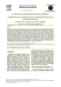
2.3 Biological Database Biological databases act as libraries of life science information which are collected across the world from scientists and also scientific experiments. In the 1980’s there were primary database projects that were developed (Racheli & Roded, 2001). These databases are important to the Bioinformatics field because they make it easy to manipulate large data sets. These datasets have been integrated from multiple data sources. They also make it easy for scientists to access these resources for their own purpose, for instance, the databases have improved search sensitivity because they provide additional search options such as searching using the item number. Their efficiency makes it easy for scientists to make use of the information that is contained in those databases (Latek, 2004). Among the functions of biological databases, the provision of biological data is also available in computer readable form. Biological databases are classified into sequence and structure database. The sequence database contains nucleic acid sequences and protein sequences. Sequence databases also represent a repository for wet-lab results and primary source for experimental results. On the other hand, the structural databases only contain the protein sequences. Among the sequence databases there are databases which are widely used by Biologists around the world such as GenBank and European Molecular Biology Laboratory (EMBL). The structure databases that are also widely used such as Protein Information Resource (PIR) to sequence proteins (Racheli & Roded, 2001). GenBank was firstly built and managed by the Los Alamos National Laboratory (LANL). It was then awarded to the National Centre for Biotechnology Information (NCBI) in the 1990s (Mizrachi, 2003). The database is built to contain genomic sequences of single cell (e.g., bacteria) and multi-cell (e.g., animals) organisms which were investigated by scientists around the world. The NCBI team collected the data for this database by the submissions of sequence data from authors around the world (Benson et al., 2004). A study by Sullivan (2013) indicates that a recent report showed that these biological data bases have approximately 11, 000 submissions per day. Figure 2.1 shows the growth of the GenBank sequences after a period one month starting from February 2013 to August 2014.
14
Figure 2.1: GenBank growth graph.
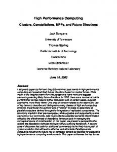
GenBank database is a collaboration of many databases, which started in the mid-1990s and became part of the international nucleotide sequence database collaboration. Among those collaborated databases there is EMBL database, Genome sequence database and the DNA Data Bank of Japan (DDBJ) (Mizrachi, 2003). The data in these databases are stored in flat text files which make it easier to maintain the increasing data. They are stored in a compressed form which can be viewed by File Transfer Protocol (FTP). The records in these databases are classified by their description of the sequence, the scientific name, their taxonomy of the source organism and their bibliographic references (Benson et al., 2004). There are different divisions that are found in the GenBank database which includes Expressed Sequence tag (EST), Sequence – Tagged sites (STSs) and High-Throughput Genomic (HTG). Figure 2.2 illustrates the flat text file record example, with all the information needed.
15
Figure 2.2: flat text files record (Benson et al., 2004).
The use of these flat files is because these files can be viewed on any platform without specialized software. There are about 140,000 named organisms that are being stored in the GenBank databases (Benson et al., 2004). Moreover, the complete genomes can be found on the NCBI website (Genome, 2014). European Molecular Biology Laboratory (EMBL) – Is a DNA sequence database from European Bioinformatics Institute (Racheli & Roded, 2001). This database is part of an international collaboration with DDBJ and GenBank (Kulikova et al., 2004). This database includes several sequences from different sources such as genome sequence projects. The EMBL database contains several retrieval tools such as BLAST and FASTA for sequence based retrieval (Kulikova et al., 2004). Protein Information Resource (PIR) – This is a protein database that contains various types of proteins where their primary structure are known (George, 1994). The PIR database is the first protein database which is developed by Margaret Dayhoff (George, 1994). One of the functions of the PIR is that it also contains some information about those proteins such as name and classification of the protein. Furthermore, it shows the functions and characteristics of the known proteins. It is a public database that can be accessed over the internet. This database is located in the Georgetown University Medical Centre (Protein-InformationResource, 2014).
16
2.4 Sequence alignment algorithms This section focuses on the first implemented sequence alignment algorithms and their examples so as to see the fundamentals of the algorithms.
2.4.1 Needleman-Wunsch algorithm The Needleman-Wunsch algorithm was first published in 1970 by Saul Needleman and Christian Wunsch (Martins et al., 2001). The main idea was to build the best alignment by using the optimal alignment of smaller subsequences in the search. This algorithm uses the global alignment method on two sequences and it is an example of dynamic programming (Vej, 2007). The algorithm follows three steps which are initialization of the score matrix, calculation of scores and filling the traceback matrix and deducing the alignment from the trace back matrix. The score is calculated as follows:
M(i,j) = max (Mi-1,j-1 + S (Ai, Bj) Mi-1,j + gap Mi,j-1 + gap)…………………….(1) Where the gap is the penalty and the function S returns the score for the matching of the two similarities. Gaps are made to achieve best results and there is a penalty for gaps. Gaps are calculated as follows:
p(g) = - d – (g -1)e…………………………………………………(2) Where e and d are constants, but they depend on the application that is used such as local alignment or global alignment. The next step on this algorithm is to fill the scores in the traceback matrix and later trace the path beginning from the lower right-hand corner of the table. The following example illustrates this algorithm with all the steps that are required. This was taken on the tutorial that was done in Brigham Young University (SequenceAlignment, 2013). The sequences that is used for this example are as follows: GAATTCAGTTA (sequence #1) GGATCGA (sequence #2) So Si,j = 1 for the match score Si,j = 0 for the mismatch score W = gap penalty
17
Initialization: This step creates a matrix M + 1 column and N + 1 row, then the first row and column must be filled with zeros as follows.
The next step is to fill the matrix as follows:
The rest of the matrix is filled as follows:
Fill in column 2
18
Fill column 3
The final matrix
By filling up the matrix of the two sequences the results of the full matrix is the above diagram. Traceback step: The traceback step starts at the very last cell of the matrix and look at direct predecessors as follows:
19
2.4.2 Smith-Waterman algorithm The Smith-Waterman algorithm was proposed in 1981 ( Vej, 2007). Unlike the NeedlemanWunsch algorithm, this algorithm uses the local alignment method. This algorithm tries to find the similar regions between the two sequences. It is also an example of the dynamic programming. The difference between these two algorithms is that the scoring matrix cells are set to zero, which has no gaps and is illustrated by equeation 3:
…………………………………………..(3) Where Hi j is the maximum similarity of the two segments ending in ai and bj respectively. The similarity of residues ai and bj is given by a weight matrix considering match, substitution or insertion/deletion. The following example illustrates Smith-Waterman algorithm but all the
20
steps involved are the same as Needleman-Wunsch algorithm. Smith-Waterman algorithm example was taken from a tutorial that was done for advanced dynamic programming (Dynamic-Programming, 2010). The sequences that are used for this example are as follows: A A T G T (sequence #1) A T G A C (sequence #2) Initialization: Scoring Metric: So Si,j = 1 for the match score Si,j = -1 for the mismatch score Gap = -2 Maximum of possible scores: 0 + s (A, A) = 0 + 1 = 1 0 - g = 0 - 2 = -2 0 - g = 0 - 2 = -2 0 (no pointer)
This process is repeated until all the cells are filled and the final matrix is as follows:
21
After this step the traceback step follows and it begins with the maximum scoring cell. At this point, what is left is to construct the alignment from traceback path.
Local Alignment AATGT Show in blue
ATGAC
2.5 High Performance Computing (HPC) HPC can be defined as a collection of hardware and software techniques developed for building computer systems capable of performing large amounts of computation faster than a usual computer. Middleton (2011) also provides a definition of HPC and says it is a computing environment which applies supercomputers and computer clusters to address complex computational requirements. HPC architecture includes computers, networks, and algorithms require a conducive environment for making it usable. The supercomputer can be described by its performance, which includes speed, power and scalability. This kind of technology can be applied in many fields such as Material Science, Bioinformatics, Brain Science and Climate Modelling (Sosa, 2011). HPC was introduced in the early 1960’s by Seymour Cray at Control Data Corporation (CDC) (Sosa, 2011). The CDC 6600 was built in 1964 and had a speed of 40 MHz- 3 MFLOP/s. The memory was faster than the CPU and it
22
was used for weather forecast (Defusco, 2014). Figure 2.3 shows the first supercomputer ever built in 1964.
Figure 2.3: CDC 6600 (Defusco, 2014).
This technology grew in the 1970’s using a few processors, in the 1990’s supercomputers with thousands of processors were built (Cortada, 2013). By the 20th century the technology of parallel supercomputers appeared with thousands of processors. Now in the 21st century supercomputers use over 10,000 processors such as CPU, GPU, which are connected by fast networks (Cortada, 2013). Figure 2.4 shows the HPC timeline where the idea started and how it will look like in 2020.
23
Figure 2.4: HPC Timeline (Probert, 2013).
2.5.1 Parallel computing Parallel computing is a way of dividing a large job into several tasks and uses more than one processor simultaneously to perform these tasks (Nakano, 2012). It can also be defined as a form of computation in which many calculations are carried out concurrently. These calculations are divided into smaller ones which can then be solved concurrently. There is a consensus among the computer developers that the importance of parallel computing and the development of parallel computing have been very rapid. This technology has been used because it has the following advantages: Solve larger problems. Faster turn-around time. Overcome limiting to serial computing. Cheap components to achieve high performance.
2.5.2 HPC architectures There are a number of HPC architectures which are used nowadays and these are as follows: Symmetric multiprocessors – It is a type of HPC architecture which multiple processors share the same memory, but its disadvantage it that it is more expensive and is less scalable.
24
Vector Processors – It is a type of HPC architecture where the CPU is optimized to perform well with arrays or vectors, this architecture has a high performance. Cluster computing – Is a concept where a set of loosely connected computers work together so they can be logically viewed as one computer. This technique is used in distributed systems where there are computers connected together and they share computing tasks assigned to the system (Cortada, 2013). These connected computers communicate using network to pass messages between them. Clusters consist of computers, switches which are used for the communication. A cluster consists of two component nodes, namely, the master node and the computing node and these are connected using a switch. A master node can be configured with a full Linux installation, it then distributes computing tasks to the other computing nodes in the cluster. Master node is in control of all computing nodes and provides a single point of administration for the whole cluster. Nodes communicate across a private network and the tasks are divided among them by a master node. The compute node carries out the computational tasks assigned to it by the job scheduler. Figure 2.5 shows all the cluster components.
Figure 2.5: Cluster Computing environment (Cortada, 2013 ).
Clusters are mostly used these days because they have high performance, price ratio, guarantee of usability and have a lower maintenance cost (Georgiev, 2009). The software’s for the clusters are open source software components. There are many of types of cluster such as fail-over clusters, load-balancing clusters and High performance clusters and these are discussed below.
25
Fail-over clusters: This type of cluster consists of a group of independent computers which are connected via a local network and are linked together by cluster software. They operate by moving resources between the nodes to provide service if system components fail (Highleyman, 2010). Load-balancing clusters: This type of cluster is usually used in web sites which have a high traffic, whereby several nodes host the same site. Then a request for a web page is dynamically routed to nodes that have a lower load. This is a critical issue that is faced in parallel computing to ensure fast processing and efficient utilization (Guo & Bhuyan, 2006). High performance clusters: This type of cluster is used to run parallel programs for time intensive computations and it uses computer clusters to address complex computational principles.
2.6 High Performance Computing (HPC) in South Africa. In South Africa there is a centre that is responsible for HPC that started in 2007 (van Rooyen et al., 2007). The centre is funded by the Department of Science and Technology which aims to produce world-class HPC that enables research with high impact on the South African Economy. The main objective of the HPC centre is to enable South Africa to become globally competitive and speed up the Africa’s socio-economic upliftment. The centre aims to help the industries and also universities in their research. Furthermore, the HPC has also provided significant commercial opportunities for South Africa to participate in cutting-edge research into big data processing (UKTI-Digital, 2014). The most demanding users for CHPC’s resources is the South African National Biodiversity Institute (SANBI) which was founded in 1996 (Conveny-Computer-Corparation, 2007). The SANBI is the largest Bioinformatics research facility in South Africa. SANBI uses the CHPC facilities when their internal HPC resources are flooded. For instance, Bioinformaticians at SANBI are currently using the Convey systems to study Venturia inaequalis which is a fungus that attack apples (Conveny-Computer-Corparation, 2007). The centre of HPC is planning to expand the usage of the Convey system in areas such as Human Language Technologies (HLT), researchers seek to promote the use of HLT to improve digital communication among the 2 000 languages in Africa (Conveny-ComputerCorparation, 2007). One of the goals of the centre is to enhance computational research
26
across all academic disciplines which will result in improved social and economic conditions in South Africa (Conveny-Computer-Corparation, 2007). Mvelase et al. (2013) looks at the South Africa’s cloud facilities and states that it is used by small enterprises that doesn’t afford the costs of Information and Communication Technology (ICT) infrastructure. Cloud facilities are attractive to those owners of small business, but government is facing a big challenge that affects the economy and ability to deliver core services to citizens. Mvelase et al. (2013), states that as the benefits of egovernmence are clear , but even though these benefits are clear there are some challenges that platform creates. Mvelase et al. (2013) further states that the cloud computing for egovernment can reduce Information Technology (IT) labour costs and provide needed scalability (Mvelase et al., 2013). For Mvelase et al. (2013) there was too little work done regarding the implementation of the e-government applications in South Africa (Mvelase et al., 2013). Mvelase et al. (2013) proposed a framework for developing a public government cloud for South Africa to support e-government. The framework includes Cloud Program Management officer (CPMO), Cloud Consumers, Cloud Providers, Cloud Auditor and Security and Data Privacy. South Africa has clouds that already exist, such as IBM’s VMware’s and cloud computing for medical research that is used in University of Pretoria (Mvelase et al., 2013).
2.7 Timeline of work done in sequence alignment algorithms This section focuses on the early developed sequence alignment algorithms and shows how the evolution of the field of HPC merged to create the most powerful algorithms and that can handle the flow of high through-put data.
2.7.1 From 1980 – 1990 In 1982 Michael Waterman introduced an algorithm that applies dynamic programming techniques to obtain optimal sequence alignment (Waterman, 1983). Waterman described that there are sets of weights that must be assigned to mismatches, insertion/deletions. Waterman further claims that sometimes there are unknown constraints on the sequence that causes the true alignment to disagree with the computer solution (Waterman, 1983). This algorithm is developed to overcome these problems by producing all alignments within a specified distance of the optimum. The distance can be chosen after the optimum is computed and the alignment can be repeated (Waterman, 1983). Waterman further alludes that when
27
problems are solved where the initial optimum takes significant time and storage, the Kth best-path method of operation are not easy to implement (Waterman, 1983). For the experiments, the algorithm is restricted to single insertion/deletions. The distance between A and B Waterman set a matrix D and initialized by Dk,0 = k( 0
k
n) and D0,l = l( 0
l
m). The values are obtained by Di,j = min {Di-1,j + d(ai, Δ), Di-1,j-1 + d(ai,bJ), Dij-1 + d(Δ ,bj)}. Waterman illustrates this by taking A = A-U-A-A-A and B = A-U-G-G-AA-A, where matches have 0 weight while mismatches and insertion/deletions have a weight of 1 (Waterman, 1983). Table 2.1 shows the resulting D and traceback. Table 2.1: Traceback diagram (Waterman, 1983).
The traceback algorithm is based on the reasoning that an alignment score can be decomposed into three parts which are the score to the current position (Ti, j), the weight of the next step (d (,)), and the score of the remaining alignment. Waterman (1983) further made some experiments on the α and β chains of the chicken hemoglobin (Waterman, 1983). For this experiment the insertion/deletions lengths are increased. The results of this experiment indicates the size of neighborhoods, there is 14 alignments with 0% of the optimum, 14 within 1%, 35 within 2%, 157 within 3%, 579 within 4%, and 1,317 within 5% (Waterman 1983). In 1989 Randall Smith and Temple Smith developed a computer algorithm that could extract the pattern of conserved primary sequence elements common to all members of homologous protein family (Smith & Smith, 1990). This algorithm also falls under dynamic programming method. Smith and Smith (1990) state that there is a major challenge in molecular biology, which is the identification of important amino acid sequence elements that encode functional domains of proteins. Smith and Smith (1990) further highlights that although the x-ray structure analysis is the most direct method, sequence comparative methods are far easier and mostly used. This method involves clustering the pairwise similarity scores among a set of related sequences to generate a binary tree. The algorithm is extended from dynamic programming algorithm of Smith and Waterman to generate sequence patterns from locally
28
optimal pairwise alignments. This modification enables the resulting patterns to be used as an input sequence for subsequent pairwise alignment. The major extension to the dynamic programming algorithm involved rules which have four establishments as follows (Smith & Smith, 1990): For a gap of length k, a length-independent plus a length-dependent gap penalty (W1 + W2*k) (11, 12) is imposed upon the initial introduction of a gap in an alignment. No gap penalty is applied for the insertion of a single-residue-length gap across from a previous gapped position in a pattern. Only the length-dependent penalty, W2*k, is applied when extending a gap adjacent to a gap character in either of the sequences being aligned. The alignment of a gap character with any other character has a match score of 0. The pattern construction methodology applies to all families of closely related sequences in the NBRF/RIP release database (Smith & Smith, 1990). For enabling the entire database to be clustered efficiently, Smith performed the pairwise match score between all sequences that are in the database, which are generated using a high speed hash algorithm (Smith & Smith, 1990). Figure 2.6 shows the sequence alignment results generated by cluster, the AACC pattern generated from cluster 50
Figure 2.6: (A) sequence alignment results generated by cluster, (B) AACC pattern generated from cluster 50 (Smith & Smith, 1990).
Smith states that even though the sequential pairwise alignments were used rather than a single optimal multi-sequence alignment during pattern construction, the algorithm cannot guarantee that the final pattern is optimal for the entire set (Smith & Smith, 1990).
29
In 1990 Altschul et al. (1990) came up with a new approach to the rapid sequence comparison tool called BLAST. This tool is developed based on the word method. This approach directly approximates alignments that optimize a measure of local similarity (Altschul et al., 1990). The algorithm is described to be simple and robust. BLAST can be implemented in a number of ways and can also be applied in a variety of contexts such as gene identification, protein sequence database searches and motif searches (Altschul et al., 1990). The most studied measures are those used in conjunction with a variety of the dynamic programming algorithm. These methods assign scores to insertions, deletions and replacements to compute an alignment of two sequences that corresponds to the least costly set of mutation (Altschul et al., 1990). BLAST employs a measure based on well-defined mutation scores and directly estimates the results that would be obtained by a dynamic programming algorithm for optimizing this measure. The method detects weak, but biologically significant sequence similarities and is more than an order of magnitude faster than existing heuristic algorithms (Altschul et al., 1990). This method is evaluated based on performance with random sequences, the choice of word length and threshold parameters (Altschul et al., 1990). Figure 2.7 shows the probability q of BLAST missing a random maximal segment pair as a function of its score S (Altschul et al., 1990).
Figure 2.7: Probability q of BLAST (Altschul et al., 1990).
BLAST approach permits the construction of extremely fast programs for database searching. The main advantage of BLAST is the amenability to mathematical analysis which can be a valuable tool for the molecular biologist (Altschul et al., 1990).
30
2.7.2 From 1991- 2000 The cryptogene-gRNA algorithm: This algorithm was developed by Michael Waterman and Arndt Haeseler for sequencing cryptogenes (Waterman & Haeseler, 1993). This is a dynamic programming algorithm to search for unknown cryptogenes and for the sequences that model the editing of gRNA. This research shows that the nucleic acid sequence database is rapidly increasing, doubling approximately every two years (Waterman & Haeseler, 1993). The goal of the algorithm is to modify existing algorithms so that it can gain observation into a newly discovered biological phenomenon. The algorithm detects possible gRNA genes and cryptogenes among genomic DNA (Waterman & Haeseler, 1993). The key insight of this algorithm is to allow the free insertion of U into potential cryptogenes to increase the number of base pairs with the potential gRNA. Waterman and Haeseler (1993) claimed that cryptogene-gRNA algorithm is similar to the Smith and Waterman algorithm. Waterman modified Smith-Waterman algorithm to make cryptogene-gRNA algorithm suitable for finding cryptogenes. Waterman describes that the reason to employ local algorithms such as Smith-Waterman is the unknown locations of cryptogenes (Waterman & Haeseler, 1993). Waterman describes some features that are employed, which are based on the search as follows: There must be at least five base pairs in the anchor. There cannot be more than three G.U base pairs in the anchor. There must be at least four adjacent Watson-Crick base pairs in the anchor. The number of adjacent inserted U’s cannot exceed eight. Between inserted U’s there cannot be more than three (non-edited) base pairs at the 5’ end of the cryptogene. These rules have improved the results in the last column, which are shown in Table 2.2, but they are not good enough to suggest that it can find unknown cryptogene-gRNA pairs reported Waterman (Waterman & Haeseler, 1993).
31
Table 2.2: Ranking by score of known gRNA when searching the maxi circle with four cryptogenes (Waterman & Haeseler, 1993).
The Combinatorial Extension (CE) algorithm: The new algorithm was developed by Ilya Shindyalov and Philip Bourne which builds an alignment between two protein structures (Shindyalov & Bourne, 1998). The CE algorithm involves combinatorial extension of an alignment path defined by aligned fragment pairs rather than conventional techniques using dynamic programming and Monte Carlo optimization (Shindyalov & Bourne, 1998). Shindyalov and Bourne (1998) report that this algorithm is fast, robust and accurate in finding an optimal 3D structure alignment and is suitable for database scanning and detailed analysis of large protein families. Shindyalov and Bourne (1998) further states that this algorithm is tested and compared with results from Dali and Vast using a representative sample of similar structures. The alignment path is constructed from aligned fragment pairs (AFPs) of fixed size m, which is one fragment length m from the first protein and another fragment from another protein to form a pair. The main goal of the alignment is to empirically determine the best values for parameters used in a combinatorial extension based structure comparison to balance accuracy and sensitivity against computational cost (Shindyalov & Bourne, 1998). Table 2.3 shows the results that are found using three algorithms which are CE, Dali and VAST.
32
Table 2.3 : Similarities obtained by CE and not detected by Dali and VAST (Shindyalov & Bourne, 1998).
Table 2.4 shows the comparison of structure alignments for 10 difficult structures obtained by these three methods. Table 2.4: Results obtained by CE, Dali and VAST in 10 difficult structures (Shindyalov & Bourne, 1998).
The T-Coffee algorithm: Notredame et al. (2000) introduced a new algorithm in 2000 which was called T-Coffee algorithm for multiple sequence alignment. This method is broadly based on the popular progressive method approach to multiple alignments ( Notredame et al., 2000). T-Coffee algorithm avoids the most serious pitfalls that are caused by the greedy nature of the algorithm. The two main features of the algorithm: Provides a simple and flexible means of generating multiple alignments using heterogeneous data sources. It is used to find the multiple alignments that best fit the pairwise alignment in the input library
33
The data provided to the algorithm is from the library of pairwise alignment. Notredame et al. (2000) uses a BaliBase database of multiple sequence alignments to test for accuracy. In addition, most of the 141 protein alignments in the database used in the test case are three dimensional structures. These BaliBase alignments according to Notredame et al. (2000) are constructed by manual structure comparison and validated using structure-superposition algorithms such as DALI. Figure 2.8 shows the comparison between T-Coffee and Prrp.
Figure 2.8: Comparison between T-Coffee and Prrp ( Notredame et al., 2000).
Notredame et al. (2000) further commented that T-Coffee is implemented in ANSI C and runs on a Linux platform with Pentium II processors (330 MHz). Table 2.5 shows results of T-Coffee compared with other multiple sequence alignment methods. Table 2.5: T-Coffee vs other multiple sequence alignment methods ( Notredame et al., 2000).
Notredame et al. (2000) concludes by describing T-Coffee as the combination of local and global information (Notredame et al., 2000).
34
2.7.3 From 2001- 2010 The Genetic algorithm: The algorithm was developed by Yokoyama et al. (2001) in 2001, which is applied to an extensive area of the genome sequence analysis (Yokoyama et al., 2001). This algorithm is based on the iterative method. Yokoyama et al. (2001) posit that this algorithm is one of the reliable approaches to align multiple sequences. The algorithm is developed and used in the program called MAGA which is accessible on the web. The algorithm has some new features which are as follows: Crossover- It is a process performed by coupling the right half of alignment 1 to the left half of alignment 2, where the alignments 1 and 2 are high-scoring alignments selected from the alignment groups obtained in the previous step. Two new mutations- The first one is ―gap annihilation‖, this sweeps away gaps from the alignment. As a consequence, this mutation leads to decrement of the number of gaps. The second one is ―gap unification‖, this unifies two gaps into one gap, hence this mutation works to decrease the number of gap groups. Figure 2.9 shows these two mutations:
Figure 2.9: (A) gap annihilation and (B) gap unification mutations (Yokoyama et al., 2001).
The performance of the algorithm is tested using BaliBase for the MAGA program against two versions of ClustalW which are version 1.7 and 1.8 (Yokoyama et al., 2001). Table 2.6 shows the results obtained in the performance test: Table 2.6: Performance test between MAGA and ClustalW version 1.7 and 1.8 (Yokoyama et al., 2001).
35
Yokoyama et al. (2001) reports that MAGA takes about one to two hours to construct the multiple alignments for one of the protein families that are listed in the Table 2.6, using the PC with AMD Athlon CPU (800 MHz) and 256 Mbytes memory. In the near future, it is expected that the program will have new features by which a user not only uses amino acid substitution matrix prepared, but they can prepare their own (Yokoyama et al., 2001). The data-parallel algorithm: This algorithm was developed by Andrew Mueller et al. (2006) at the University of Indiana in 2003. The algorithm was developed for classic comparative genomics algorithm, the dot plot along with a multiprocessor extension (Mueller et al., 2006). Data-parallel algorithm is based on the dot matrix method. Moreover, Mueller et al. (2006) states that the dot plot algorithm is still the only algorithm for computing a full direct pairwise comparison between two sequences (Mueller et al., 2006). As a result, the increase in the size and availability of genomic data has led to the expansion of commodity microprocessors to include high performance feature sets. The improved version of the dot plot algorithm removes the runtime dependency reported Mueller et al. (2006). The new algorithm first computes a score vector for each letter in the alphabet against the horizontal sequence q (Mueller et al., 2006). The new version of the algorithm has a running time of O (|q||s|) which increases the space requirements to |∑ ||q|. Mueller et al. (2006) reports that this increase can be managed for all genomics comparisons where |∑DNA | = 4 (Mueller et al., 2006)The data-parallel processors allow the same operation to be applied in parallel to all the values stored in a vector register (Mueller et al., 2006). The algorithm is extended by blocking the resulting matrix by dividing q into equal sized column blocks for each processor, this is done to support multiple processors. For the performance test a set of models that contained the core operations of the algorithm are developed, they are used initially to help understand the implementation parameters (Mueller et al., 2006). The dataparallel algorithm implementation have two versions that are used to gauge the performance, these two versions are both standard versions (Mueller et al., 2006). The platform that is used to implement and test the algorithm is an Apple dual PC with the following features as pointed out below: 2 GHz PowerPC. 3.5 GB DDR SDRAM running OS X 10.3.5. g++ 3.3 compiler for the code. Velocity Engine (ADC 2004). Version 1.31 of the Boost library.
36
The complete genomes from the mitochondrial genome database and others are used for development, testing and benchmarking (Mueller et al., 2006). Table 2.7 shows the results for the performance of the model. Table 2.7: Performance results (Mueller et al., 2006).
Table 2.8 shows the results of the sequence size and the time it took to compare at 1850 Mops. Table 2.8: Sequence size v’s the time it took to compare at 1850 Mops (Mueller et al., 2006).
The algorithm development demonstrates the feasibility of directly comparing large genomic sequences (Mueller et al., 2006).
2.8 Sequence alignment algorithms timeline This part gives a detailed timeline on the sequence alignment algorithms where there are matrices that are followed such as the type of the problems that are solved, type of the algorithm whether it is a pairwise or multiple algorithm. There are three main criteria on which all the sequence alignment algorithms are judged on, these criteria include speed, accuracy and memory. Out of all the those criteria, accuracy is the most important. This section further illustrates the computers that are used in some of the algorithms, some of the publications have left out to describe the computers or clusters that are used in the research.
37
The need to describe the material that is used is that the emerging field of high performance computing is more concerned on the performance of the algorithms together with the performance of the cluster towards that algorithm. The contributions of the algorithms towards finding the best algorithm are discussed. The evolution of sequence alignment algorithms are of interest because it started by using man made materials to align the sequences. As the technology improves, computers are developed to solve complex problems. These computers are not that efficient as the databases are increasing with sequences. The HPC came to the rescue by building systems that will be dedicated to solving big data problems. As the algorithms are investigated, there are matrices that are targeted to be important in the evolution of the algorithms. The matrices that are listed contributed to the evolution of sequence alignment algorithms. Type of problem: This matric focused on types of problems that are solved in each algorithm analysed. These problems are taken from the literature review of the evolution of sequence alignment algorithms. Type of algorithm: This specified whether the algorithm is suitable for pairwise alignment or multiple sequence alignment or both. The speed of the algorithm: This deals with the performance of the algorithm as a whole and which machines are being used. The contribution of each sequence alignment algorithm in the evolution: This focuses
on each algorithm and its contribution in the evolution. Table 2.9 addresses the evolution of the sequence alignment algorithms towards the high performance computing field
38
Table 2.9: Sequence Alignment Timeline
Name Of the Algorithm or Research name.
Year Developed.
Type Of problem researched.
Type of algorithm and the material used.
Contribution of the algorithm in the evolution.
There are difficulties when applying dynamical programming techniques to obtain optimal sequence alignments. The problem is in identifying essential amino acid sequence elements that encode functional domain proteins
It is a dynamic programming algorithm.
The problem that the algorithm faces is to create a rapid sequence comparison The problem that is approached by CE is to build an algorithm that aligns two protein structures This algorithm is facing a problem with generating accurate alignments automatically.
The algorithm accommodates for both pairwise and multiple sequence alignments. This algorithm accommodates for pairwise alignments
This algorithm contributed by giving the users can produce all alignments within a specified a distance of optimum Given this particular similarity matrix and gap scoring scheme, for any single pair of amino acid sequences and/or patterns, the present method will find the optimal AACC pattern The algorithm is robust and simple and it can be used in a variety of contexts.
Sequence alignments in the neighbourhood of the optimum with general application to dynamic programming. Automatic generation of primary sequence patterns.
1982
BLAST
1990
The combinatorial extension (CE) algorithm.
1998
The T-Coffee algorithm
2000
The algorithm
Genetic
2001
The algorithm is solving a genome sequence analysis problem
The data-parallel algorithm
2003
The problem that is dealt with is on the direct pairwise comparison between two sequences
1989
39
It is a dynamic programming algorithm that deals with pairwise alignments.
It is a multiple sequence alignment algorithm. This algorithm runs on Linux platform with Pentium II processors (330 MHz) It is a multiple sequence alignment algorithm, using the PC with AMD Athlon CPU (800 MHz) and 256 Mbytes memory. The algorithm is developed for classic comparative genomics in direct pairwise comparison. The Apple dual 2 GHz Power PC, 3.5 GB DDR SDRAM running OS X 10.3.5
The algorithm produced accurate results in finding an optimal alignment fast. T-Coffee is the combination of local and global information; it provides a simple and flexible means of generating multiple alignments. This algorithm is one of the reliable approaches to align multiple sequences, it is hosted on the web server for easy use and a simple interface Data-parallel and multiprocessor implementation of the dot plot algorithm, demonstrated some of the challenges in developing high performance software to handle very large data sets.
2.9 High Performance Computing in Sequence Alignment The parallel centre star algorithm: As the sequences increase exponentially and algorithms are being developed for handling this influx of data, the multiple sequence alignment is still the most problematic area in computational molecular biology (Sahoo et al., 2009). This algorithm is based on the dynamic programming. Sahoo et al. (2009) introduced a parallel centre star algorithm in 2009 to solve the problem with regard to time consumption. This algorithm is implemented on a Symmetric MultiProcessor (SMP) cluster using Message Passing Interface (MPI) library functions (Sahoo et al., 2009). The architecture is based on a Master-Slave approach and all messages are controlled by the MPI library. The algorithm that Sahoo et al. (2009) implemented uses C++ programming and the MPI library. The environment that the algorithm runs is a 4 node cluster, each node has 2.4GHz Intel Pentium-IV, 512 MB RAM running under Red Hat Linux (Sahoo et al., 2009) . The nodes are connected with one gigabits/s Ethernet switch and the algorithm is tested using the running time, which includes execution time, communication overhead and reading input data from a file (Sahoo et al., 2009). Table 2.10 shows the time comparison of a sequential centre star algorithm versus parallel centre star algorithm. Table 2.10: Time comparison between sequential centre star algorithm versus parallel centre star algorithm (Sahoo et al., 2009).
The experiments that are performed aim at how the numbers of the sequences affect the performance of the system and other experiments aimed at how the processing time is affected as the lengths of sequences grow (Sahoo et al., 2009). Figure 2.10 shows the results obtained.
40
Figure 2.10: Running time of sequential and parallel algorithm using 4 processors for 8 Kbps sequence length (Sahoo et al., 2009).
2.9.1 From 2011- 2013 Hosny et al. (2011) proposed a solution to find the optimal alignment of the huge DNA sequences where the solution uses the sequence size in megabyte-scale instead of kilobytes (Hosny et al., 2011). Hosny et al. (2011) state that the challenge of the metrics such as the functionality, performance, storage and hardware cost which can lead to an efficient solution for the sequence alignment problem (Hosny et al., 2011). For example, the solution proposed is implemented using C++ and OpenMP and tested using an 8-core CPU of 1.6MHz and 4MB cache memory. The RAM of the CPU is 4GB and running on Windows Server 2007. The visual studio 2010 software is used in the development and the nucleotides of exact sizes from 32K to 5M are generated from measuring the scalability. The Smith-Waterman algorithm score parameters are used in the tests and a storage space is 50 GB. Figure 2.11 shows the results in speedup and efficiency that is obtained for the parallel execution with different number of workers.
41
Figure 2.11: Speedup and efficiency Results on different number of workers (Hosny et al., 2011).
Isa et al. (2012) proposed a novel efficient hardware architecture to optimize the execution time of Dynamic Programming-based (DP) pairwise sequence alignment algorithms in hardware. Isa et al. (2012) also proposed a new metric as an independent performance to evaluate and compare different core implementations on different Field Programmable Gate Array (FPGA) platforms (Isa et al., 2012). The proposed core is useful in processing long sequences whereby it is not possible to allocate enough processing elements on the available FPGA devices (Isa et al., 2012). In addition, Isa et al. (2012) uses a fixed number of configuration elements regardless of the folding factor. Isa et al. (2012) proposed that the core is implemented on an Alpha data ADM-XRC-5LX card with a Virtex 5 vlx110 FPGA on it, the UniProtKB/ TrEMBL database is used and it consumed 2.3 GB of memory. The implementations are done on an Intel(R) Quad Core 64-bit Q8300 with 2.50 GHz processor and 4.00GB of RAM. The results show that the core achieves over 40% normalized speed-up compared to the state of the art with the speed-up growing directly with the number of folds. Accordingly, Settle (2013) also implements the Smith Waterman algorithm for DNA or protein sequences using dynamic programming on FPGA with OpenCL (Settle, 2013). These sequences are in a manner readily familiar to both hardware and software developers. The settle’s implementation is based on the Novo-G and the sequences are stored one element per byte, the nucleotides are stored in a four significant bit.
42
The experiments are performed using the task kernel executing on a Nallatech PCIe-385n board in an HP Z620 workstation which is running Windows 7 Professional 64-bit. Settle used m = 1259197 elements of a megavirus’s complete genome as a database sequence. The performance of the Smith Waterman algorithm is measured in Cell Updates Per Second (CUPS). The FPGA resource utilization for the task based Smith Waterman kernel is recorded. The unidirectional linear systolic array of Smith Waterman processing elements consumed 0.23% of logic, 0.10% of register and 0.01% of memory blocks per processing element. The overall overhead is 22% for logic, 7.9% for register and 12% of memory blocks (Settle, 2013). Table 2.11 shows the results of FPGA performance and power efficiency. Table 2.11: FPGA Performance and Power Efficiency (Settle, 2013).
Settle further shows that for n = 256, CPUs achieved 2.5 GCUPS running at 0.038 GCUPS/W while the GPUs reached 9.4 GCUPS with power efficiency of 0.067 GCUPS/W (Settle, 2013).
2.10 Related work on High Performance Computing (HPC) Fan et al. (2004) proposed to use a cluster of Graphics Processing Unit (GPU) for high performance computing where a parallel flow simulation was developed using the Lattice Boltzmann Model (LBM). The LBM developed on a GPU cluster and have simulated the dispersion of airborne contaminants in the Times Square area in New York City (Fan et al., 2004). The developed GPU cluster GPU cluster had two purposes, firstly was for graphics and computation. The second purpose was for visualization and interpretation of large capacity datasets (Fan et al., 2004). The GPU cluster has 32 nodes connected by 1 Gigabit Ethernet switch where each node was equipped with HP PC that have two Pentium Xeon 2.4GHz processors and 2.5GB memory. The GPU cluster produced 832 GFlops for a theoretical performance, the whole GPU cluster cost was $ 136,000 (Fan et al., 2004). The addition of 32 GPUs to a CPU cluster for computation increased the theoretical peak performance by 512 GFlops at a cost of $ 12,768.
43
The GPU cluster simulation computed 15.6 M LBM cells in 0.317 second/step and also simulated the transport of airborne contaminants in the Times Square area of New York City. According to Fan et al. (2004), simulation results in the Times Square area of New York City, where the 3.8 meters/lattice spacing resolution is used to simulate the area and the performance is 0.31 second/step on 30 nodes. Hu and Evans
developed a Power and Environment Awareness Module (PEAM) for
Beowulf clusters (Hu & Evans, 2009). The development of the PEAM addresses the issues that the Beowulf clusters encounter such as heat-inducted hardware failure, which makes large scale commodity clusters fail frequently. However, the cost effectiveness of Beowulf clusters is challenged by lack of adapting its power state according to varying workload (Hu & Evans, 2009). The PEAM module is developed on a Beowulf cluster at Purdue University, which aimed at reducing the operating cost and increase the reliability of the cluster by reducing heat generation and optimizing workload distribution in an environment aware manner (Hu & Evans, 2009). The PEAM module is also developed to achieve the environment awareness by directing jobs to those nodes with the lowest temperature, which will increase the reliability of the Beowulf clusters. To test the PEAM module on the Beowulf cluster the temperature of different cluster rooms is recorded at different times and the monitoring system is deployed to record the reading. These readings are recorded at different temperatures and they show a great difference. Hu and Evans (2009) found that the failure rate of compute node doubles with every 10°C increase in temperature. The PEAM module is implemented as a software module in Muai scheduler and the environment awareness workload can be reduced up to 40% for some workloads. Chien et al. (1997) worked on the High Performance Virtual Machine (HPVM) project, which provides software that enables high performance computing. It is done in clusters of PCs and workstations, where using standard supercomputer Application Programming Interface (API) such as MPI, Global Arrays and SHMEM Put/Get. The project’s aim is to unify these models to deliver high performance parallel computing, on shared heterogeneous resources (Chien et al., 1997). The challenges that are critical in the project are delivering high performance communication to standard high level API’s, coordinating scheduling, resource management, and managing heterogeneity (Chien et al., 1997). Chien et al. (1997) first developed Fast Message (FM) version 1.1 which performed well on the latency and
44
bandwidth micro benchmarks
(Chien et al., 1997). Unfortunately, FM 1.1 had some
problems that are noted below: The fact that they allowed control over when communication data is processed, but not how much data is processed. The cost of copying a user-specified buffer merely to prepared a header to it before passing the data to FM. The cost of copying data from FM's internal buffer into a messaging layer buffer and then into the user-specified buffer. To address the problems encountered by the first version Chien et al. (1997) redesigned the FM interface so that it could support data spacing and streamed messages (Chien et al., 1997). Chien et al. (1997) developed a second version of the FM on SPARC stations. They deployed their work on a 32 node cluster 2way symmetric multiprocessor Pentium Pro machines in Illinois (Chien et al., 1997). Chien and Prusakova demonstrates the performance of high performance Virtual Machines using Zeus-MP which is a hydrodynamics code produced by the Cosmology NSF Grand Challenge team. The demonstration is done on different platforms such as Cray T90, Cray T3D etc., Figure 2.12 represents the performance of HPVM (Chien et al., 1997).
Figure 2.12: Zeus-MP on a variety of hardware platforms (Chien et al., 1997).
45
Hsu and Feng (2005) conducted a feasibility analysis of power awareness in commodity based high performance clusters (Hsu & Feng, 2005). Their study revolves around a 16 processor Opteron-based Beowulf cluster. The Beowulf cluster is configured as four nodes of quad processors. The study shows that a 5 % performance slowdown can be traded off for an average of 19% system energy which is saving and 24% system power reduction (Hsu & Feng, 2005). Hsu and Feng (2005) further stated that power efficiency is the most critical part of developing cost-effective, small-footprint clusters. Thus, Hsu and Feng (2005) performed various tests such as benchmark tests of different software’s are performed to compare power consumption between them. The HPL and NAS MPI benchmarks are compared so as to see which can save power. Hsu and Feng used system wattage to evaluate power awareness on the cluster, the results showed that on average processor wattage consumes about 77 watts and accounts for 69% of the total system wattage (Hsu & Feng, 2005). Boukerche et al. (2006) propose to build High- Availability (HA) clusters based model for high performance computing. Boukerche et al. (2006), further propose to investigate the hardware and management layers of the HA-HPC cluster design together with the parallel application layer. Boukerche et al. (2006) states that one of the challenges in a clustered environment is to keep system failure to minimum levels and achieve the highest possible level of system availability ( Boukerche et al., 2006). Boukerche et al. (2006) analyzed a small scale HA-HPC functionality and performance, the evaluation was performed on an eight node cluster . Each of the nodes was equipped with a Pentium4 3.2GHz processor 1.0GHz memory and running Linux Redhat 9.0, two of the nodes are set as master nodes which are managed by HA-Oscar. The other six nodes are configured as compute nodes and are connected by a 100MB/s network and Boukerche et al. (2006) stated that dynamic PVM and FT-MPI interfaces are used to handle the parallel jobs. For experiments, a 2600 byte script file was used to render a 1024x768 picture with an output size of 2.3MB. Boukerche et al. (2006), stated that the best performance was observed while using four nodes, but it dropped when using the eight nodes ( Boukerche et al., 2006). The results showed that the manager/worker algorithm that was proposed can be improved to suit most of the FT-MPI implementations ( Boukerche et al., 2006). The results also show that combining HPC and HA architectures is feasible in achieving HA cluster that is used for high performance computing ( Boukerche et al., 2006).
46
2.11 Conclusion This chapter introduced the research background of the dissertation and gave a detailed review of the biological databases that are used in Bioinformatics. It also introduced the first sequence alignment algorithms that were developed. Furthermore a detained review of the sequence alignment algorithms and also gave an account of how HPC in the management of big data is performed. The HPC that are used were also discussed about and a detailed review of the HPC was also given. This chapter concluded by giving a detailed sequence alignment algorithm timeline. The following chapter looks at the research methodology and implementation.
47
3 Methodology and Implementation 3.1 Introduction This chapter describes the methodology used in this dissertation and software development process involved in designing and developing a Beowulf cluster for evaluation of sequence alignment algorithms. This chapter further outlines a proposed architecture and the system requirements. The research analyses how a Beowulf cluster can be used in sequence alignment algorithms. The aim is to develop an efficient and faster Beowulf cluster to perform sequence alignment algorithms in a minimal time. The factors that affect the Beowulf cluster are also discussed in this chapter.
3.2
Research Methodology
The methodology style that was adopted in this dissertation was a mixed method. This method was selected because there was a need to go into detailed literature of the sequence alignment algorithms and also how the HPC field merge with the sequence alignment algorithms. The following methodology was used. Literature study. This part was identified in chapter two where the literature of the existing sequence alignment algorithms was investigated in details. The evolution of sequence alignment algorithms was also explained in chapter two. The introduction of HPC and their architectures was covered in chapter two. The use of HPC in handling sequence alignment algorithms was also part of the methodology where the problems in the algorithms were identified. Theoretic and practise based systems. In order to show which HPC cluster yield an increased performance at a low cost, the Beowulf cluster was chosen because of it was a low cost and managabled cluster. Proof and concept. The Beowulf cluster was developed to perform the sequence alignment algorithms and also to examine which algorithm perform best between TCoffee and Clustal-W algorithms. The following section will go in detail on the Beowulf cluster that was developed to support the objectives that are stated in chapter one
48
3.3 Proposed Cluster Architecture The proposed cluster architecture is a Beowulf cluster. This cluster is chosen because the development and maintenance is affordable. Beowulf clusters are just a collection of personal computers interconnected through a network, which operates as parallel computers. There are great advantages of using the Beowulf cluster such as: Low price to performance ratio. It is easy to expand to increase performance. Implementation with ordinary personal computers The software’s that are used are free from Linux operating system. Figure 3.1 shows a high level architecture of the Beowulf cluster.
Figure 3.1: High Level Beowulf Architecture (Chavan, 2012).
Figure 3.1 shows the final design of the cluster where users can submits jobs to the cluster. The Beowulf cluster that is developed consists of one master node and four compute nodes, a Cisco system catalyst 2960 series switch is used to connect the computers together. The logical view shows layer by layer of the cluster and a general view shows a wide scope of which of the components being connected and which hardware and software used. Figure 3.2 shows a logical view that represents the tools that are needed to develop the Beowulf cluster.
49
Figure 3.2: Logical view of the Beowulf cluster (Chavan, 2012).
3.4 Cluster requirements In building a cluster there are certain things that need to be considered such as hardware and software. For hardware part, the important things checked are computers which are of the same vendor and a switch needed to connect the computers for communication. The following section will specify the hardware and software that ware needed to develop the cluster. There are specifications of hardware that are needed for developing a Beowulf cluster, the following section deals with the hardware specifications. The Beowulf cluster consists of the off-the-shelf computers and for this dissertation the hardware that was used for developing and implementing the cluster is as follows: Proline desktop computers are used for the design and implementation. The Pentium (R) Dual-core E5200 @ 2.50 GHz, 2.50 GHz processor. RAM that will be used is 2 Gigabytes.
50
250 Gigabytes Hard Drive. A Cisco system catalyst 2960 series. After the hardware is collected and connected, there is a need for software’s that are used starting from the operating system down to the Bioinformatics software. The basic software’s needed are operating system and message passing software, the required software to perform sequence alignment are installed after the cluster is up and running.
3.5 Hardware Configuration 3.5.1 Master Node The master node acts as the heart of the cluster because it is the one that communicates with the rest of the computers, it makes the scheduling of the jobs amongst the compute nodes. In addition, this node acts as a server where it provides access to the network. The master is responsible for creating files that are used by the compute nodes for running the applications that are given to them.
3.5.2 Compute Node The compute nodes are a collection of computers that are connected by a switch for communication. These compute nodes are assigned jobs by a master node and they run those jobs and report the results to the master node. In turn, the master node then takes all the results from those nodes and builds one report that is sent to the user as an output. The compute nodes are the ones that are the majority in a cluster and are divided into two partitions. The first partition is batch and the second are interactive partitions.
3.5.3 Network For cluster components to pass messages to each other they need a network connection that will connect them. The connection is achieved by having the Network Interface Card (NIC) on each computer that is connected to a network medium. Master node has two NICs, which one of the NIC is connected to the network medium for communication with compute nodes, while the other NIC is for the outside network connection. The computers can be connected to a Hub or a switch. Figure 3.3 shows the cluster network interconnection.
51
Figure 3.3: cluster network interconnection.
The switch is used for making all the computers to pass messages to one another. The Cisco switch called Catalyst 2960 series is used for communication. The Cisco catalyst 2960 series switch has 24 ports of fast Ethernet or Gigabit desktop connectivity (Cisco, 2010). Cisco (2010) provides the following features: Fast Ethernet or Gigabit Ethernet connectivity to deliver high performance application. It provides Power over Ethernet (PoE) of up to 15.4W per port to supply power to network-attached devices. Robust security capabilities which are the most important features of the network medium. It has a quality of service intelligence which prioritizes traffic and optimizes bandwidth in the network It is easy to manage and scalable.
52
3.6 Software The system that has been designed needed some software’s that are suitable for high performance computing simulations. These software’s ranges from the operating system to sequence alignment software. The implementation of the system used the Linux kernel which consisted of GNU applications which range from servers to compilers. Operating System: The operating system that was used in the development of the cluster is Linux, which is based on Ubuntu 13.10 (Saucy Salamander) for the master node. This operating system is open source software that is free so there is no need for payment to get it and its applications are free. This operating system was chosen because it is the current stable version. This operating system allowed the installation of cluster software, which ranges from compilers to sequence alignment applications. For the computing nodes, the mini version was chosen. This is a server image without a Graphic User Interface (GUI). It integrates the Linux kernel and contains basic services such as Secure Shell (SSH), Network File System server (NFS). The compilers included are gcc, gfortran, g ++ and C++ and MPICH2 is also included. It should be noted that the unnecessary software’s for the server system are not included. Message-passing Libraries: This is a standardized system which is a portable message-passing system that is used in clusters, parallel computers and also in heterogeneous networks (Yelick, 2001). It is not a programming language, but it is used to define the syntax of the core library for the use of portable message-passing languages such as C++, C and FORTRAN. These message-passing libraries are needed when one need to perform intensive calculations, they are also used to divide and distribute independent jobs in different computers. For this research messagepassing interface was used because it is the mostly used library for the numerical analysis. Compilers: Parallel computing commonly uses certain programming languages such as C++, C, FORTRAN and Python. For this reason programming languages that are supported are integrating with compilers such as gcc and g++. After the operating systems are installed on all the computers the next step is to configure the IP addresses of all the computers. For the master node which has two NICs, the first NIC which is eth0 is used for the outside connection and it uses Dynamic Host Configuration
53
Protocol (DHCP). The second NIC is for the communication with the compute nodes in the cluster. This NIC uses static configuration. It is easy to access the nodes by their names rather than by their IP addresses. This is achieved by adding all the nodes in a host file, these IP addresses that are added are static local IP addresses. Figure 3.4 shows the hosts file.
Figure 3.4: host file diagram.
The hosts file needs to be exactly like figure 3.4 before saving the file. To check if the file is edited correctly when contacting other nodes, they must respond positively and no packets lost. The following task is to create a new user on all nodes, this is done so as to use one username for all the nodes when sending out jobs without passwords.
3.6.1 Network File System (NFS) The files and programs used for MPI jobs need to be available to all the nodes in the cluster, these files are accessed on the master node by the compute nodes. The NFS enables the mounting of the files remotely so that they can be accessed as if they are within a local directory. Within the master node a directory that is shared, needs to be created and its owner changed so that can be accessed by compute nodes. In this file the nodes that shared this directory are listed and the permission on how to use it was sought. Once the conditions are stated, the NFS server is restarted so as to update the server. Meanwhile, on the compute nodes the same directory is created and mounted with the master IP address and the directory that is shared. To prevent the mounting of the directory every time the compute nodes bootup, the fstab file is edited by adding the IP address of the node that contain the directory and also the name of the directory. When this is done the directory can be mounted successfully.
54
3.6.2 Set-up secure shell (SSH). For the cluster to work, the master node needed to communicate with compute nodes and vice versa. This communication is made possible by installing an SSH server at all nodes. Once the SSH is installed on all the nodes, the SSH is tested by logging into another node, this created a file in the SSH directory which is called unknown_hosts. The next step is to login to the user that is created and generate the keys that are distributed to all the nodes. This is done by ($ ssh-keygen) command, this created two files and the id_dsa.pub file is transferred to other nodes. Once the transfer is done, the contents of that file are copied to another file which is called authorized_keys and then it can be confirmed that the communication is successful.
3.6.3 MPICH2 The MPICH2 is built so that a number of communication infrastructures can be used, these are called devices which are most relevant for the Beowulf environment (Chavan, 2012). The MPICH 2 is an online software that is free and is a portable implementation of MPI. It uses a portable interface to process management systems, this process management is separate. The runtime for MPICH2 consist of asset of daemons such as mpd and hydra process managers. MPICH2 need to be installed on all nodes, which had the entire executable that are needed for running MPI programs. Running the MPI program on the master node will distribute the jobs to other nodes and every node has access to the program via mpiexec command. To run the MPI programs, there are three steps that needed to be followed which are listed below. Compiling the program: The first thing is to write a small code for testing the MPI which could be just a hello world using the C++ programming language. After having that file an appropriate compiler is chosen, which is linked against the MPI libraries. The file is then saved and for compiling the program the mpicc command is used ($ mpicc -o hello hello.c). The use of ―- o‖ option created the output file. Copy: The files are copied to the shared directory so that it can run on all the nodes, the shared directory also consists of the executable files that are needed to run the MPI programs. Execution of the program: Once the program is compiled and copied to the shared directory. The command that is used to run the MPI programs is mpiexec and it is
55
accompanied by ―np or n‖ which are used to specify the number of processors to be used. That argument is followed by ―-f‖ and the name of the nodes that runs the program. This is done by creating a file called hosts that listed all the nodes. To run the hello world program which uses 6 processes: $ mpiexec –np 6 –f hosts ./hello Once the program is finished running, the output results are shown in the figure 3.5.
Figure 3.5: hello World output results.
The hydra process manager is the one that is used in starting parallel jobs. This process manager can work with many daemons such as pbs and ssh. It is the default process manager for the MPICH2 version that was chosen.
3.6.4 ClustalW-MPI This software is the most popular tool for multiple sequence alignment that can be used in HPC (Kim & Joo, 2010). The alignment is achieved in three steps which are pairwise alignment, guide-tree generation and progressive alignment. This software is an MPI implementation of ClustalW and is used to test the performance of the Beowulf cluster. The aim of this test is to motivate the use of HPC in Bioinformatics field. The idea of buying specialized equipment for HPC can cost a lot of money, but using the Beowulf clustering for institutions and also industries can cut costs. The pairwise alignments can be parallelized since they are time independent of each other. The algorithm that is used by this software is a linear space profile-profile alignment.
56
The software need to be installed and after the installation is completed, it is checked if the installation is successful ($ which clustalw-mpi) command is used. Once the software is installed successfully, to test the software there is a need of a sequence that is aligned. The sequences are obtained at National Centre for Biotechnology Information (NCBI) website (Nucleotide, 2014). The format of the file is a fasta file, after the file is created it is tested by typing ($ mpirun -np 5 ./clustalw-mpi -infile=dele.input) command. This command created two additional files with ―.aln and .dnd‖ extensions, the dot aln file contained the sequence alignment of all the sequences that are aligned with ClustalW-MPI software and the dot dnd file shows the description of the sequences. It further shows the time it took to sequence the alignment and their scores. Figure 3.6 shows the test file which is created for testing the ClustalW-MPI software.
Figure 3.6: ClustalW-MPI test results.
3.6.5 T-Coffee T-Coffee is a multiple sequence alignment package that can be used to sequence biological data (Rius et al., 2010). This method is broadly based on the popular progressive method approach to multiple alignments (Rius et al., 2010). This package can align protein, DNA and RNA sequences which can be viewed in three dimensions.
It has been developed to
overcome the original method and it is based on MPI mechanism. T-Coffee 3.79 offers many
57
features than the previous versions such as the ability to have a three dimension view and additional libraries. After downloading the file, the contents are extracted and then the package is installed (Aluru-HPC-Group, 2014). For the experiments there are sizes of alignments that are prepared on the fasta file format, the sizes range from 50 Mb to 365 Mb. Those sizes are prepared for both sequence alignment algorithms because ClustalW-MPI uses the ―.input‖ file format and T-Coffee uses the ―.fasta‖ format.
3.6.6 Htop System Monitoring. The Htop system monitoring is a tool that is used in Linux to allow the users to monitor resources and the processes that are running in real-time. This software can be used to check usage per Central Process Unit (CPU) by the programs that are running. The Htop software is installed so as to check the usage of the programs that are running on the cluster. Figure 3.7 shows the output of Htop.
Figure 3.7: H-Top results.
There are varieties of factors that can affect the MPI application’s performance, factors that are of high importance are discussed below. Platform /Architecture Related: These factors are caused by the hardware parts such as operating system characteristics, network adapters, memory subsystem and the number of CPUs Network Related: These factors are caused by the connection of the cluster and also configurations that are done on the cluster. These factors can also be caused by a faulty switch, network tuning options and also the faulty cables. 58
Application Related: These factors can be caused by the applications themselves that run on the cluster such as memory usage patterns, I/O and also the message size used. Furthermore, these factors can be caused by load balancing and communication to computation ratios. MPI Implementation Related: For these, the factors can be caused by the type of packages that are chosen, this can include the message buffering, message passing protocols and routine internals.
3.6.7 Benchmarking An excellent collection of benchmarks that is used on Beowulf clusters is HPL (High Performance Linpack). This benchmark suite allows making accurate predictions on which type of computational problems that can be suitable to be solved on the particular Beowulf cluster. The benchmark measures the performance of the system, which is based on the actual performance of the cluster using different problem sizes. For the theoretical performance one can submit the hardware specifications on the HPL website so as to find the theoretical system performance (Top500-HPL-Calculator, 2014).
3.7 Conclusion This chapter discussed the research methodology and the software development process that was involved in the design and development of a Beowulf cluster for evaluation of sequence alignment algorithms. The chapter concluded by giving the factors that can affect the Beowulf cluster. In the next chapter, experimentations are done to test the performance of the cluster and also the sequence alignment algorithm performance on the Beowulf cluster.
59
4 Experiments 4.1 Introduction This chapter focuses on the performance of the cluster in different experiments. There are basic experiments that are fundamental that was performed, hence this chapter further discusses the sequence alignment algorithms that are also part of the experiment. The theoretical performance is discussed and its actual performance. To evaluate the acceptability of the designed cluster on how it performs and use the resources as required, few parallel programs are implemented. The first program that is implemented is the calculation of pi value. The second experiment is the calculation of prime numbers which have a given range. The third experiment is based on the Quad_MPI which also shows the performance of the parallel computing.
The fourth experiment involved the ring_mpi
program that is written in C programming language. The last experiment is for the standard performance is the satisfy program that is demonstrated for a particular circuit which performed an exhaustive search for solutions of the circuit satisfy problem. The experiments for sequence alignment algorithm in the Beowulf cluster are conducted. The first experiment is on the ClustalW-MPI, which is mostly used in the sequence alignment using high performance computing. The second experiment is on the T-Coffee sequence algorithm that is used to get accurate results in sequencing alignment. The Cluster standard benchmarking experiment which is used to find the performance of Top500 supercomputers is conducted. The High Performance Linpack Benchmark (HPL) is the one that is conducted so as to check whether the designed cluster is producing a reasonable performance. There are many algorithms that are used in the HPL package that checks the performance of the cluster, some of these algorithms are two-dimensional block, cyclic data distribution and panel factorization.
4.2 Pi Calculation This program calculates the π value, where π is a mathematical constant that is the ratio of a circle’s circumference to its diameter. This constant can be written as pi, which is approximately equal to 3.141590. The aim of this program is to compare the constant value of pi with the calculated value. The error that has occurred is also computed and the time that
60
is taken by the program to calculate the value of pi is displayed by the program. The difficult part is to check which part of the program needs to be executed parallel after the part is identified then the work is distributed. The size of the file is 1, 5 Kb. Figure 4.1 shows the time taken by different number of computers to calculate the value of pi.
Figure 4.1: Pi Calculation graph.
While the computation is divided among the cluster, each node reported its contribution towards the whole computation of the program. The information also showed which process is running on which node and its contribution of that node to the process that it is working with. Figure 4.2 shows how each node contributes on the cluster.
Figure 4.2: Diagram that shows the distribution of computation in the Cluster.
61
4.3 Prime Number program This is a C program that counts the number of prime numbers between 1 and N, it uses MPI to carry out the calculations in parallel computers. The algorithm that is used by this program is simple. Prime number program assumed for each integer A, it looks whether any smaller Z evenly divides it. The total amount of work for any given N value is proportional to ½*N^2. The single machine output is compared with the whole cluster output. The output shows the different N values and the time it took to find its prime numbers. Figure 4.3 shows the results of one computer against the cluster.
Figure 4.3 Prime Numbers graph
The output also showed the number of N values that are computed and the work is distributed amongst the cluster nodes equally. The master node sent out tasks to other nodes and when each node is finished it sends back the results to the master node. When all the nodes are finished the master node outputs the results
62
4.4 Quad_MPI This program approximates an integral using a quadrature rule. It uses MPI to compute the results in parallel. The estimation of an integral of f(x) from A to B is 50/ (pi*(2500*x*x+1)). A = 0.000000 B = 10.000000 N = 9999999 Exact = 0.4993633 Figure 4.4 shows the time taken by the program to combine the results.
Figure 4.4: Quad_MPI graph.
The MPI divided the computation among the processors that the cluster has and each contribution of a processor is determined. The error of the computation is also calculated. The overall time taken by the program is calculated and displayed. This explanation is illustrated in Figure 4.5.
63
Figure 4.5: Contribution of each node in the computation.
4.5 Ring_MPI This program estimates the time taken to send a vector of F double precision values through each process in a ring. Process 0 sends F double precision values to process 1, which passes them to process 2 and so on until to the last process sends back the value to process 0. The time of transmission is recorded and the process is repeated in different array sizes F. The F double precision values are random values. The different times intervals are recorded in the execution of ring_mpi program. The computations are done in parallel using MPI. Figure 4.6 shows the results of the ring_mpi.
64
Figure 4.6: Ring_mpi graph.
4.6 Circuit satisfiability Problem This program is used for a demonstration of a particular circuit that uses an exhaustive search for solutions of the circuit satisfy problem. The program uses MPI to carry out the solution in parallel. This problem assumes that a logical circuit of AND, OR and NOT gates are given, with N binary inputs and a single output. It determines all inputs which produce a 1 as the result. The general problem is not complete, so there is no known polynomial-time algorithm to resolve the general case. The natural way to search for solutions then is exhaustive search by the program. In an interesting way, this is a very risky and separate version of the problem of maximizing a scalar function of multiple variables. The difference in this instance is transparent because both the input and results only have the values 0 and 1, rather than a constant range of real values. This problem is a natural contender for parallel computation, since the separate evaluations of the circuit are completely independent. Figure 4.7 demonstrates the circuit satisfy problem in parallel computing.
65
Figure 4.7: Circuit satisfy problem.
4.7 ClustalW-MPI This software is built based on the progressive method for multiple sequence alignment algorithms (Al-neama et al., 2014). ClustalW-MPI is the tool which is mostly used for aligning multiple sequences of different types such as proteins, DNA and nucleotides. It uses MPI library and runs on parallel computers. The ClustalW-MPI is targeted on workstation clusters with distributed memory architecture. The parallelization of the distance-matrix calculations create some problems on distribution time-independent jobs to parallel computers (Al-neama et al., 2014). The ClustalW-MPI uses a scheduling called fixed-size chunking where groups of jobs of one fixed size are allocated to available processors. The data that is sequenced needs to be of ―.input ―type so it can be understood by the mpi library. Figure 4.0 shows some of the sequence that is collected on NCBI website, Figure 4.8 shows the time it took to align a sequence of data using parallel computers with is obtained using 365 Mb.
66
Figure 4.8: ClustalW-MPI graph.
After the alignment is finished the output had two files. The file which comprised of ―.aln‖ extension contained the sequenced alignment and the one with ―.dnd‖ extension had the description of the sequences.
The scoring of the groups of aligned sequences is also
outputted and also the overall score is the part of the output. Figure 4.9 shows the sequenced alignment file.
Figure 4.9: Sequence Alignment File.
67
There are also other experiments done using different file sizes of the sequences so as to check the performance of the cluster. The Table 4.1 illustrates those experiments. Table 4.1 : Total execution time for 4 sequence sizes using ClustalW-MPI.
File size (Mb) 365 170 100 50
1 Processor
2 Processors
3 Processors
4 Processors
5 Processors
1.163s 0.899s 0.062s 0.009s
4.105s 1.250s 0.284s 0.055s
6.167s 3.144s 1.582s 0.118s
8.284s 5.288s 2.647s 1.099s
9.030s 6.303s 4.225s 2.651s
4.8 ClustalW-MPI v’s T-coffee This section tries to identify the faster algorithm between ClustalW-MPI and T-coffee. The T-coffee package is the first parallel implementation of the T-coffee multiple sequence alignment tool, which is based on MPI and RMA mechanisms. This package makes it easy to run parallel jobs on a cluster. It is similar to the ClustalW-MPI package, but they differ in their output. With T-coffee there is also an html file which can show the sequenced alignment on the internet with colours that show the regions of similarity. For this experiment the same sizes that are taken for ClustalW-MPI are used to test T-Coffee tool. Table 4.2 show the results for T-Coffee. Table 4.2 : Total execution time for 4 sequence sizes using T-Coffee.
File size (Mb) 365 170 100 50
1 Processor
2 Processors
3 Processors
4 Processors
5 Processors
2.168s 1.095s 0.254s 0.448s
5.115s 2.287s 1.884s 0.947s
9.668s 6.526s 3.254s 2.487s
11.582s 9.471s 6.954s 3.941s
15.775s 12.668s 8.854s 5.547s
Figure 4.10 illustrates the time it took for ClustalW-MPI and T-coffee to align the same sequence. Both of the files are 365 Mb size. T-Coffee took more time than ClustalW-MPI to produce the results, but the output is more accurate than the ClustalW-MPI.
68
Figure 4.10: ClustalW-MPI v’s T-coffee.
Figure 4.11 shows the results of T-Coffee html file that was obtained when the experiments were done. This file shows the regions where there is a high similarity between the aligned sequences.
Figure 4.11: The html results from T-Coffee.
69
4.9 Theoretical Peak Performance in a Cluster The theoretical performance of the cluster is not based on the actual performance that is obtained from a benchmark test, but it depends on the cluster specification to determine the peak rate of execution of floating point operation for the computer. To calculate the theoretical peak performance of the cluster, the master node peak is calculated and then multiplied the node performance by the number of the nodes that the cluster had. The following is the standard formula used for node theoretical peak performance: Node performance in GFlops = (CPU speed in GHz) x (number of CPU cores) x (CPU instruction per cycle) x (number of CPUs per node). For cluster: CPUs based on Intel Premium(R) E5200 (2.50GHz, 2-cores): 2.50 * 2 * 4 = 10 GFlops CPU speed in GHz: 2.50 No. of cores per CPU: 2 No. of instructions per cycle: 2 Five PC Clusters Theoretical Peak Performance: 10 GFlops * 5 = 50 GFlops
4.10 Benchmarking The Benchmarking is good for the verification of the performance of the cluster. This can be done by running the accepted benchmarks for Top500 supercomputers. The purpose of the benchmark is to compare the theoretical peak performance with the actual performance of the cluster. The HPL is a software package that solves a dense linear system of equations in double precision architecture on distributed memory computers. The performance of the cluster is measured using this package on numerous computers and forms the basis for the Top500 supercomputers list. For running the tests HPL needed to be installed on the cluster so it can work. After it is installed on the shared file on the master node and the executable files are
70
built, the next step is to modify the input data file called HPL.dat. The file must be in the same directory as the executable files. The file contained information about the problem size, computer configuration, and the algorithm that is executed. The file contains 31 lines long, where some of the lines needed to be modified to suit the user. Figure 4.12 is an example of the HPL.dat file of the cluster.
Figure 4.12: HPL.dat file.
To run the HPL on a cluster, the make file must exist in all the nodes and the command to run HPL is $ mpiexec –np x. /xhpl, where x is the number of cores in the cluster. Figure 4.13 shows the HPL results on the cluster.
71
Figure 4.13: HPL results.
These sets of experiments are done and the observations are noted which are discussed in the results and discussion chapter. The highest value in the HPL experiment is 9.90 GFlops, which showed that there is an absolute performance gain in cluster over a single computer. The efficiency of the cluster is 19.8 %, which is a surprise, but given the various limitations in the cluster it is perhaps not that surprising to get such value. This effect is caused by less processor speed and low memory of the computers that are used to build the cluster. The theoretical test can also be done online, where it rates the cluster performance from the Top500 supercomputers. The HPL calculator can be accessed on the website (Top500-HPLCalculator, 2014). Based on the HPL calculator the efficiency of the cluster is 83.3%, but it is not on the Top500 supercomputers list.
4.11 Conclusion This chapter gave an insight on the experiments that were performed in the Beowulf cluster to measure the actual performance of the cluster using different experiments and different sizes of problems. Furthermore, it continued by giving the sequence alignment algorithm experiments in Beowulf cluster and concluded by giving HPL experiments. In the next chapter the results that were obtained on the experiments are discussed in detail.
72
5 Results and Discussion 5.1 Introduction This chapter discusses the results that were observed in the experiments done to test the Beowulf cluster. A comparison of the sequence alignment algorithms that were tested practically including theoretical statements is also discussed. Furthermore, the sequence alignment algorithm timeline and the contribution of each algorithm in the hierarchy are discussed. The challenges encountered during the implementation of the Beowulf cluster are also discussed, including the benefits of using the cluster
5.2 Results from the experiments Clusters can reduce the overall computation time, this part will discuss the observed results of the experiments that were performed. Less computation and intensive computation experiments are also discussed and their effects are discussed.
5.2.1 Less Computation Experiments observations and performance Less computation experiments performed showed that jobs with less computation tasks such as Ring_mpi and Prime Numbers experiments, when the numbers of processors are increased the performance time takes longer than in a single processor. Their communication time is bounded and because the sequential runtime is so small, the time to send and receive from the master node makes the programs take a longer time with more nodes. The results showed that this delay is caused by the time to distribute the work and the time for the master node to collect the results. Such programs can also be performed on a single computer, but this is done to show that how the cluster handles less computation programs. The significance of these experiments was to find out which experiments are suitable for the cluster since less computation programs can also be executed. However, it was discovered that the problems lies with the fact that with clusters there is the communication between nodes that tends to take a long time
73
5.2.2 Intensive Computation experiments observations and performance
Intensive computation experiments such as Quad_MPI on the cluster are bounded by sequential computation time just like in less computational experiments, but with more processors the communication factor also takes over.
Because the sequential time for
intensive computation experiments is also large this is the advantage of the cluster to scale better than the less computational experiments. Experiments with more computation require more memory and space so this part is handled well by the cluster because their memory and space are distributed. When the same experiments were executed on a single PC there was an error message saying that it is out of memory because of the low memory used as compared to the cluster, therefore the whole process was aborted.
5.2.3 Results from ClustalW-MPI against T-Coffee The experiments were conducted to see which algorithm produced results in a minimal time and also which has the most reliable results in the sequences. The ClustalW-MPI scaled well and generated results in a minimal time as compared with T-Coffee. The experiments were done using different file sizes so as to see the performance of the cluster in handling big data files. The findings of the research revealed that with bigger file sizes, the communication is lesser than for the files with a lesser size. This effect caused the small sized files to communicate more and the computation becomes lesser. T-Coffee algorithm took longer time to output the results as observed in chapter four, but with the results there were also three files created which contained information about the aligned sequences, in those files there was also an html file that shows the regions of similarities have the same colour. Although the T-Coffee algorithm took longer time than ClustalW-MPI, this was also confirmed in the literature review that T-Coffee produces more reasonable results than ClustalW. The reason why T-Coffee took more time than ClustalWMPI was that with T-Coffee have huge memory requirements for the extended libraries so as to maintain the consistency in the alignment. As it was observed in Figure 3.6 and Figure 4.11 that have the scores for alignments, T-Coffee had the high score that ClustalW-MPI algorithm. This finding revealed that even though T-Coffee takes a longer time than ClustalW-MPI, T-Coffee yields accurate results than ClustalW-MPI. Similarly, the finding of this study support research done by Do et al. (2005) which revealed that T-Coffee has the most accurate results than ClustalW. These authors showed that T74
Coffee takes more time to complete than ClustalW, even though it produces accurate results it strains the CPU memory and take longer (Do et al., 2005). Edgar (2004) also did a research on these algorithms and others using the different databases. In his findings, he noted that T-Coffee yields better results than ClustalW. He also showed that ClustalW was faster than T-Coffee. As the sequences that were tested increases, the TCoffee algorithm took even longer and it was aborted because it takes much longer time (Edgar, 2004). Notredame et al. (200) also supports the results that were observed, which also support that T-Coffee yields more accurate results than ClustalW in each BaliBase category. Notredame et al. (2000) also argues that the difference between traditional progressive methods and TCoffee is that, it uses position-specific scoring instead of substitution matrix for aligning the sequences.
5.2.4 Results on Sequence Alignment Algorithm Timeline The results of sequence alignment algorithm which are supported by Table 2.9 clearly showed that the evolution of the algorithms is significant in the study of Bioinformatics because without the algorithm, there would be many problems in justifying their theories. It would also be very much difficult to predict the inheritance and also make the comparative analysis by inspection. As the algorithms become complex and advanced they tend to use more computing power which is another problem that would need some research. The use of HPC techniques to solve the problem in computation power was also investigated in this research which shows a huge contribution in handling the algorithms. Almost all sequence alignment algorithm needs fast processing computers. With the increasing availability of cheaper and faster computers, more researchers are interested in reaping the technological benefits. There is no upper boundary to the needs of computer processing power; even with the rapid increase in power, the demand is considerably more than what is available.
5.3 Efficiency of the Cluster The efficiency of the cluster, which was 19.8%, was unexpected because the predicted efficiency was 83.3%, which was found in the cluster calculator. This huge difference was because of the condition of the computers that were used. The processors that were installed
75
on each node were 2.50 GHz but the experiments took a longer time to produce results. Even though all the nodes contained 2 Gbytes of memory, at some point where the data was increased to 500 Mb there was an error saying out of memory. This error was because of the number of processes allocated on each node. The factor that was taken note of was that with the network speed of 100 Mbps, the exchange of information between all the nodes were taking longer time and some of the applications were not installed because of the security measures. In the case of a cluster, the dataset may be required to reside in memory alongside with the messaging traffic meant for the other processors. The memory plays a huge part in the efficiency and in the development of the cluster.
5.3.1 Factors that affected the performance of the Cluster Some of the effects that were stated in chapter three also played a role in the efficiency of the cluster. Furthermore, looking at the MPI, there were a number of factors that were encountered such as the message size, process number and running processes. For the message size which played a very important part on MPI application performance, this effect can be influenced by the latency and the number of processors. On the other hand, for experiments that had intensive computation such as Quad_MPI yielded a better performance because sending smaller size messages with more computation increases the performance of the application. Adding another node on the cluster can reduce the computation time, but increase the communication time. This was observed when increasing the number of nodes for experimentations. When there were many nodes, it was observed that the processes running on the cluster resulted in the delay of the production of results.
5.4 Conclusion This chapter gave a detailed discussion of the experiments that were performed on a Beowulf cluster. It continued by analysing the results of the experiments starting from the less computation experiments to intensive computation experiments. The foregoing chapter further discussed the sequence alignment algorithm results. The chapter was concluded by highlighting the factors that were affecting the performance of the Beowulf cluster. In the next chapter the conclusion and also future work is discussed.
76
6 Conclusion and Future work 6.1 Introduction This chapter begins with a research overview and research contributions of the work done on the research. The research objectives are discussed and problems that were encountered during the research are also highlighted. Finally, the recommendations that can be incorporated to improve some of the problems encountered are given.
6.2 Research overview This research study has developed and produced a Beowulf cluster system that can be used to evaluate sequence alignment algorithms. The Beowulf cluster can be used for many other things such as network simulations, environmental modelling simulations, image processing and graphics rendering. The Beowulf cluster was developed using free open source software that are available on the internet, starting from the operating system to the sequence alignment software. The Beowulf cluster was tested for performance and 19.8% efficiency was noted which was reasonable based on the network speed of 100Mbps. The less computation experiments performed less as expected because of longer communication time occurred.
6.3 Research contributions This research has through a well-defined methodological approach design and developed a Beowulf cluster for evaluation of sequence alignment algorithms. This was achieved by reviewing the available HPC architectures. A detailed sequence alignment algorithm timeline which indicates the evolution of sequences to improve the way the clusters perform is also presented. Furthermore, this research provided experiments that were performed on a Beowulf cluster to measure the performance. As a result, these experiments showed that programs with less computation take longer time than programs with intensive computation. Therefore, the factors that affected a Beowulf cluster were addressed in chapter three. The sequence alignment algorithms were performed successfully using a Beowulf cluster and a faster algorithm was identified and is the ClustaW-MPI. With the sequence alignment
77
algorithms, experiments revealed a more accurate algorithm which is T-Coffee and was slower than ClastalW-MPI.
6.4 Addressing the Research Objectives This section revisits the research objectives that were highlighted in the introduction chapter and discuss how these objectives were addressed. There are six objectives that were stated in the dissertation: Objective 1: Investigate the evolution of sequence alignment algorithms.
During the research one of the most important aspects was to investigate the evolution of the sequence alignment algorithms, this was done by collecting the literature review and journals that are based on the development of such algorithms. As it was drafted there were matrices that were identified which are most important in the evolution of these algorithms. Some of the noted matrices were the problems that each algorithm was trying to solve and how it was solved. Furthermore the equipment that was used in solving those problems were noted. The contribution of each algorithm towards the evolution of sequence alignment was also one of the matrices. This objective was done in two chapter, which are chapter one and two. Objective 2: Investigate the High performance computing techniques. The aim of this objective was to investigate and identify a suitable, cost-effective platform, but also to produce results that are comparable to high-end production clusters when running the algorithms on the system. The Beowulf cluster was chosen from the variety of other platforms because it met the requirements of the development of the system that run the algorithms. This was showed in chapter three where the advantages of the cluster were stated.The Beowulf cluster was suitable for the budget of the research and also for running program sizes starting from 50kb to 365 Mb of space. Objective 3: Design and implementation of the Beowulf cluster. The fundamental aim of this study was to have a working cluster suitable for the investigation of different factors that affect the cluster performance. This objective was performed in chapter three.These factors range from the hardware that was used to applications that were used for sequence alignment. A fully functional Beowulf
78
cluster was developed and tested. Free and Open Source Software were utilized for the software stack of the cluster. Among those software’s that were installed the most important software was the MPI because it was the one that was responsible for passing the messages to compute nodes. The SSH was also important because it enabled the passing of information without asking for passwords all the time when the information was to be distributed. Objective 4: Test and determine the baseline performance of the Beowulf cluster. The testing of the system was in chapter four and was done by using Linpack, one of the industry recommended software in HPC for testing the system and the performance. A series of experiments were performed before the sequence alignment algorithms were tested to make sure that the system was fit for handling them. This objective was successful and the algorithms performed well on the system.
The Linpack highest score was 9.90 GFlops which was convincing based on the 2 Gigabyte memory that was installed in each computer on the cluster. The theoretical performance was 50.0 GFlops. This difference was explained based on the factors that affected the cluster. One of the most important factors was the network part because of the network speed of 100Mbps that was used was so low. Objective 5 – Test the performance of ClustalW-MPI over T-Coffee software, these software acts as test-bed. The sequence alignment software acted as a test bed for the cluster that was built. This was done to support the usage of cluster in complex problems. The ClustalW-MPI had a maximum time of 9.030s using all the nodes and it was a 365Mb size file. The smallest file with sequences was 50 Kb and the maximum speed was 2.651s. For TCoffee the maximum time of 15.775s using all the nodes and the file size was 365Mb. T-Coffee took 5.547s to execute 50Kb file size of the sequences.
As it was observed T-Coffee took longer time than ClustalW-MPI, but T-Coffee produced accurate alignments as compared with ClustalW-MPI. T-Coffee based on the popular progressive method approach to multiple alignments and ClustalW-MPI is also based on progressive method.
79
Objective 6: Develop a timeline for the sequence alignment algorithms.
During the research the evolution of these algorithms needed to be documented as the field of high performance computing emerged to find solutions on how to handle such algorithms and also considers the performance of the system. This objective was performed in chapter two.The use of the timeline was to find out the importance of high performance computing in the improvement of the performance of these algorithms in the environments they are used to. This objective is linked to objective three because all the information that populated the table was extracted literature review.
6.5 Challenges Encountered The first and foremost challenge that was encountered was the funding of the equipment because to buy new equipment would cost so much, the department offered its old computers to do the research project. The second challenge was that this research is a combination of Computer Science and Bioinformatics, designing and developing a Beowulf cluster and performing the sequences was a big challenge because the researcher didn’t have a strong background of Bioinformatics. The third challenge was the technologies that are used in HPC to build such systems. When the cluster was fully developed there were problems in configuring the network and the public network had a firewall that blocked some of the applications. A greater challenge was to find the sequence data which were to be aligned by the algorithms that were chosen and some of the databases required the use of registered users only.
6.6 Future Work
As the network technology advances with time and the equipment is getting cheaper to users and, a new computing model called Grid computing is found. Grid computing is a collection of computer resources from many different locations to reach a common goal. It provides users a single point of access which is just a website interface to these distributed resources. The main goal of Grid computing is to provide a service-oriented infrastructure that
80
influences standardized protocols and facilities to enable pervasive access to, and synchronized sharing of geographically distributed hardware, software and information resources. The users of the grid can submit as many jobs as they can without being concerned about where their jobs will run. The grid may range from single systems to supercomputer farm that uses thousands of processors. Deploying some of the applications that will handle check the idle computers so that the work can be distributed to them. Another thing that could be done is to install an application that would detect faulty clusters and contact the administrator for the details. A sequence alignment algorithm that would be fast and utilize little space of the processors can be developed with the help of the evolution timeline obtained in the literature review. For speeding up the cluster one has to consider the following strategies because they can be helpful in producing a high speed in the cluster. Less communication: This means that for a cluster to be fast the initial communication must be done. In the initial communication, all the necessary information that will be needed must be supplied so that there won’t be additional information that will be needed. For example, this means that all the information must be in the same code. More Computation: This means that there should be more computation than communication between the nodes because the less communication the more there will be computation. This arises the optimization concept because if the code is handled correctly, the computations will be faster than before. Faster network connections: If there is a faster network, which means that the
communication and message passing will be faster. As a result, the infiniband switches are recommended which can have a maximum speed of 100Gbps.
6.7 Conclusion This chapter has given an overview of the research and also the contributions that were made by this research. It further addressed the objectives and how they were accomplished. Furthermore, it looked at the problems that were encountered and it concluded by giving the future work that can be extended from this research
81
References Al-neama, M.W., Reda, N.M. & Ghaleb, F.F.M. (2014). An Improved Distance Matrix Computation Algorithm for Multicore Clusters. BioMed Research International. Altschul, S.F., Gish, W., Miller, W., Myers, E.W. & Lipman, D.J. (1990). Basic local alignment search tool. Journal of molecular biology, 215 (3): 403–410. Aluru-HPC-Group. (2014). Parallel T-Coffee, Available at: http://alurusun.ece.iastate.edu/doku.php?id=parallel-tcoffee#download [Accessed April 5, 2014]. Autenrieth, F., Isralewitz, B., Luthey-Schulten, Z., Sethi, A., & Pogorelov, T. (2005). Bioinformatics and sequence alignment. Beckman Institute for Advanced Science and Technology, 1(1), 1-29 Baldauf, S.L. (2003). Phylogeny for the faint of heart: a tutorial. Trends in genetics: TIG, 19 (6), pp. 345–51. Available at: http://www.ncbi.nlm.nih.gov/pubmed/12801728 [Accessed August 6, 2013]. Benson, D. A., Karsch-Mizrachi, I., Lipman, D. J., Ostell, J., & Wheeler, D. L. (2004). GenBank: update. Nucleic acids research, 32(Database issue), D23. Boukerche, A., Al-Shaikh, R., & Notare, M. S. M. (2006, April). Towards building a highlyavailable cluster based model for high performance computing. In Parallel and Distributed Processing Symposium, 2006. IPDPS 2006. 20th International (pp. 8-pp). IEEE. Carr, J. (2008). Introduction to linux clustering, http://www.jethrocarr.com/wpcontent/uploads/2010/09/introduction_linux_clustering_1.1.pdf
1–33.
Retrieved
from
Carroll, H., Beckstead, W., O'Connor, T., Ebbert, M., Clement, M., Snell, Q., & McClellan, D. (2007). DNA reference alignment benchmarks based on tertiary structure of encoded proteins. Bioinformatics, 23(19), 2648-2649. Chavan, S. (2012). Design and Implementation of High Performance Computing Cluster for Educational Purpose.Masters dissertation.Pune: Pune Institute of Computer Technology Chien, A. A., Pakin, S., Lauria, M., Buchanan, M., Hane, K., Giannini, L. A., & Prusakova, J. (1997, March). High Performance Virtual Machines (HPVM'S): Clusters with Supercomputing API's and Performance. In PPSC Cisco. (2010). Cisco Catalyst 2960-S and 2960 Series Switches with LAN Lite Software Scalable Network Management and Enhanced Security for Growing Small and MediumSized Businesses. , pp.1–13.
82
Clustalw-mpi. (2014). MPI-distributed global sequence alignment with ClustalW. Available at: https://packages.debian.org/stable/clustalw-mpi [Accessed March 3, 2014]. Cohen, J. (2004). Bioinformatics—an introduction for computer scientists. ACM Computing Surveys (CSUR), 36(2), 122-158. Conveny-Computer-Corparation. (2007). Developing an Advanced Cyberinfrastructure. Available at: http://www.conveycomputer.com/files/7013/5593/9864/CHPC.pdf [Accessed January 27, 2014] Cortada, M.O. (2013). High performance computing on biological sequence aligment. Doctoral dissertation. Lleida: University of Lleida Defusco, A. (2014). CS1645 Using a Supercomputer, University of Pittsburgh. Do, C.B., Mahabhashyam, M.S.P., Brudno, M. & Batzoglou, S. (2005). ProbCons : Probabilistic consistency-based multiple sequence alignment.Genome research, 15(2), 330– 340. Dynamic-Programming. (2010). Dynamic Programming. , pp.1–16. Available at: http://www.biomol.it/unictbiolmol-lab/figure_didattica/04.dynamicprogrammictutorial.pdf [Accessed July 30, 1014]. Edgar, R. C. (2004, August). MUSCLE: Multiple sequence alignment with improved accuracy and speed. In Computational Systems Bioinformatics Conference, 2004. CSB 2004. Proceedings. 2004 IEEE (pp. 728-729). IEEE. Fan, Z., Qiu, F., Kaufman, A., & Yoakum-Stover, S. (2004, November). GPU cluster for high performance computing. In Proceedings of the 2004 ACM/IEEE conference on Supercomputing (p. 47). IEEE Computer Society. Genome. (2014). Genome. Available at: http://www.ncbi.nlm.nih.gov/Genomes/index.html [Accessed January 20, 2014]. George, D.G. (1994). Protein Sequence Database ( PSD ) Database Definition Document. National Biomedical Research, 1- 79. Georgiev, S., 2009. Evaluation of Cluster Middleware in a Heterogeneous Computing Environment. Masters dissertation.Linz: Austria Girke, T. (2011). Microarray Analysis The Basics.University of California,Riverside. Guo, J., & Bhuyan, L. N. (2006). Load balancing in a cluster-based web server for multimedia applications. Parallel and Distributed Systems, IEEE Transactions on, 17(11), 1321-1334.
83
Highleyman, W. (2010). Windows Server Failover Clustering: Microsoft White Paper; April 2009.[Online] Available from: http://www.availabilitydigest.com/public_articles/0504/microsoft_cluster.pdf [Accessed 09 April 2014] Hosny, A. M., Shedeed, H. A., Hussein, A. S., & Tolba, M. F. (2011, November). An efficient solution for aligning huge DNA sequences. InComputer Engineering & Systems (ICCES), 2011 International Conference on(pp. 295-300). IEEE. Hovatta, I., Kimppa, K., Lehmussola, A., Pasanen, T., Saarela, J., Saarikko, I., ... & Wong, G. (2005). DNA microarray data analysis. CSC, 2nd edn., Scientific Computing Ltd. Hsu, C. H., & Feng, W. C. (2005, September). A feasibility analysis of power awareness in commodity-based high-performance clusters. In Cluster Computing, 2005. IEEE International (pp. 1-10). IEEE. Hu, F. & Evans, J.J. (2009). Power and environment aware control of Beowulf clusters.Cluster Computing, 12(3), pp.299–308. Huson, D. (2005). Algorithmic Bioinformatics , pp.4–18. Available http://lectures.molgen.mpg.de/Algorithmische_Bioinformatik_WS0607/reinert1.pdf [Accessed 11 April 2014]
at:
Huson, D. (2009). Pairwise alignment Sequence formats. , pp.8–24. Available at: http://ab.inf.uni-tuebingen.de/teaching/ss09/gbi/script/02-pairwise-alignment.pdf [Accessed 11 April 2014] Isa, M. N., Benkrid, K., & Clayton, T. (2012). Efficient architecture and scheduling technique for pairwise sequence alignment. ACM SIGARCH Computer Architecture News, 40(4), 2631. Jiang, T. & Yu, W. (2010). A Layer-Based Approach to Multiple Sequences Alignment, paper presented at the Eighth Asia Pacific Bioinformatics Conference, Bangalore, India, 1821 January 2010, Available at: http://cs.nyu.edu/parida/APBC2010/poster_abstracts/8.pdf Kanehisa, M. & Bork, P. (2003). Bioinformatics in the post-sequence era. , 33(march), pp.305–310. Available at: http://www.bioinformatics.iusb.edu/pdf_files/kanehisa.pdf. Kasibhatla, A. (2010). A brief introduction to Dynamic Programming (DP), University of California, Los Angeles Kim, T. & Joo, H. (2010). ClustalXeed: a GUI-based grid computation version for high performance and terabyte size multiple sequence alignment. BMC bioinformatics, 11, p.467. Available at: http://www.pubmedcentral.nih.gov/articlerender.fcgi?artid=2949895&tool=pmcentrez&rende rtype=abstract.
84
Kulikova, T., Aldebert, P., Althorpe, N., Baker, W., Bates, K., Browne, P., van den Broek, A., Cochrane, G., Duggan, K., Eberhardt, R., Faruque, N., Garcia-Pastor, M., Harte, N., Kanz, C., Leinonen, R., Lin, Q., Lombard, V., Lopez, R., Mancuso, R., McHale, M., Nardone, F., Silventoinen, V., Stoehr, P., Stoesser, G., Tuli, M.A., Tzouvara, K., Vaughan, R., Wu, D., Zhu, W. & Apweiler, R. (2004). The EMBL Nucleotide Sequence Database. Nucleic acids research, 32(Database issue): D27–30. http://www.pubmedcentral.nih.gov/articlerender.fcgi?artid=308854&tool=pmcentrez&render type=abstract 22 May 2013. Latek, R. (2004). Relational Databases for Biologists : Efficiently Managing and Manipulating Your Data, Whitehead Institute for Biomedical Research. Lupyan, D., Leo-macias, A. & Ortiz, A.R. (2005). Structural bioinformatics A new progressive-iterative algorithm for multiple structure alignment. , 21(15), pp.3255–3263. Luscombe, N. M., Greenbaum, D., & Gerstein, M. (2001). What is bioinformatics? An introduction and overview. Yearbook of Medical Informatics, 1, 83-99. Manohar, P. & Singh, S. (2012). Protein Sequence Alignment : A Review. , World Applied Programming journal, 2(March), pp.141–145, Martins, W. S., del Cuvillo, J., Useche, F. J., Theobald, K. B., & Gao, G. R. (2001, January). A multithreaded parallel implementation of a dynamic programming algorithm for sequence comparison. In Pacific Symposium on Biocomputing (Vol. 6, pp. 311-322). Mavromatis, K., Ivanova, N. N., Chen, I. M. A., Szeto, E., Markowitz, V. M., & Kyrpides, N. C. (2009). The DOE-JGI Standard operating procedure for the annotations of microbial genomes. Standards in genomic sciences, 1(1), 63. Mizrachi, I. (2003). GenBank : The Nucleotide Sequence Database. Nucleic acids research, pp.1–14. mpich. (2014). Index of /static/downloads. http://www.mpich.org/static/downloads/ [Accessed February 20, 2014].
Available
at:
Mueller, C., Dalkilic, M. M., & Lumsdaine, A. (2006). High-performance direct pairwise comparison of large genomic sequences. Parallel and Distributed Systems, IEEE Transactions on, 17(8), 764-772. Mvelase, P. S., Dlamini, I. Z., Sithole, H. M., & Dlodlo, N. (2013). Towards a government public cloud model: The case of South Africa. International Conferences on High Performance Computing. Nakano, J. (2012). Parallel computing techniques. In Handbook of computational statistics (pp. 243-271). Springer Berlin Heidelberg.
85
Notredame, C., Higgins, D. G., & Heringa, J. (2000). T-Coffee: A novel method for fast and accurate multiple sequence alignment. Journal of molecular biology, 302(1), 205-217. Nucleotide. (2014). Nucleotide Search database. Available at: http://www.ncbi.nlm.nih.gov/nuccore/?term=human full genome [Accessed April 3, 2014]. Phillips, A.J. (2006). Homology assessment and molecular sequence alignment. Journal of biomedical informatics, 39(1), pp.18–33. Available at: http://www.ncbi.nlm.nih.gov/pubmed/16380300 [Accessed August 7, 2013]. Probert, M. (2013). High Performance Computing - History of the Supercomputer. Available at:http://www-users.york.ac.uk/7B0BF9F0-5EF5-4758-96879DFBECFADB8A/FinalDownload/DownloadIdC91700D3B47DFE9BEE7232BCEE93E1CD/7B0BF9F0-5EF5-4758-96879DFBECFADB8A/~mijp1/teaching/4th_year_HPC/lecture_notes/History_of_Supercomputer s.pdf [ Accessed February 18,2013]. Protein-Information-Resource. (2014). Protein Information Resource. Available at: http://www.pir.georgetown.edu/ [Accessed January 31, 2014]. Quackenbush, J. (2001). Computational analysis of microarray data. Nature reviews genetics, 2(6), 418-427. Rhee, S. Y., Dickerson, J., & Xu, D. (2006). Bioinformatics and its applications in plant biology. Annu. Rev. Plant Biol., 57, 335-360. Rius, J., Orobitg, M., Cores, F., Solsona, F., Mcgilvary, G., van Hemert, J. I., ... & Atkinson, M. (2010). Analyzing Parallel T-Coffee: a Parallel Multiple Sequence Aligner. Van Rooyen, B., Sikwane, B., Lowies, P., Gcukumana, M. (2007). Reaping competitive advantage through high performance computing and data curation fast facts, CSIR publications, 33–43. Racheli, Z and Roded, S (2001). Algorithms for Molecular Biology: Bioinformatics Databases and Tools, Tel Aviv University: Ramat Aviv. Rosenberg, M.S. (2007). Sequence Alignment: Concepts and History.Tempe: Arizona State University , pp.155–185. Rumbold, A. (2004). Multiple sequence alignment algorithms for the phylogenic analysis of chloroplast DNA .Honours thesis, University of Tasmania. Rust, A. G., Mongin, E., & Birney, E. (2002). Genome annotation techniques: new approaches and challenges. Drug discovery today, 7(11), S70-S76.
86
Sahoo, B., Kumar, A., & Padhy, S. (2009). Parallel Implementation of Centre Star Method in SMP Cluster for Multiple Sequence Alignment. Int. J. of Recent Trends in Engineering and Technology, 2(1). Schaffer, J. D., Dimitrova, N., & Zhang, M. (2006). Bioinformatics. In Advances in Health care Technology Care Shaping the Future of Medical (pp. 421-438). Springer Netherlands. Sequence-Alignment. (2013). Merrily We Clustal Along Sequence Alignment. Available at: http://bioinformatics.byu.edu/A8FB9B26-AEEB-45EC-8F6CD19C3E78F3B8/FinalDownload/DownloadIdC7B93860A9C5B33549EAFE57C9972606/A8FB9B26-AEEB-45EC-8F6CD19C3E78F3B8/portals/54/images/Home/Presentation.pdf. Settle, S.O. (2013). High-performance Dynamic Programming on FPGAs with OpenCL. Available at: http://ieee-hpec.org/2013/index_htm_files/29-High-performance-Settle2876089.pdf [Accessed February 19, 2014] Settles, B. ( 2008). Lecture 2 Sequence Alignment Sequence Alignment . Available at: http://pages.cs.wisc.edu/~bsettles/ibs08/lectures/02-alignment.pdf [Accessed March 26, 2014] Shindyalov, I. N., & Bourne, P. E. (1998). Protein structure alignment by incremental combinatorial extension (CE) of the optimal path. Protein engineering, 11(9), 739-747. Smith, R. F., & Smith, T. F. (1990). Automatic generation of primary sequence patterns from sets of related protein sequences. Proceedings of the National Academy of Sciences, 87(1), 118-122. Sosa, C.P. (2011). HPC: Past, Present, and Future. IBM & Biomedical Informatics and Computational Biology: University of Minnesota Rochester Stein, L. (2001). Genome annotation: from sequence to biology. Nature reviews genetics, 2(7), 493-503. Strengholt, B. (2013). Acceleration of the Smith-Waterman algorithm for DNA sequence alignment using an FPGA platform. Bachelor thesis. Delft: Delft University of Technology Sullivan, D.G. (2013). CS 105 GenBank : A Database of Genetic Sequence Data. Boston University Boston, Massachusetts. Top500-HPL-Calculator. (2014). Top500 HPL Calculator. Available at: http://hplcalculator.sourceforge.net/ [Accessed April 20, 2014]. Tse, H. T. K., Meng, P., Gossett, D. R., Irturk, A., Kastner, R., & Di Carlo, D. (2011). Strategies for implementing hardware-assisted high-throughput cellular image analysis. Journal of the Association for Laboratory Automation, 16(6), 422-430
87
UKTI-Digital. (2014). South Africa: High Performance Computing January 2014 - Open to Export. Available at: http://opentoexport.com/article/south-africa-high-performancecomputing-january-2014/ [Accessed April 9, 2014]. Vej, G.W. (2007). Bioinformatics Explained Bioinformatics Explained. Available at: http://www.montefiore.ulg.ac.be/~kvansteen/GBIO0009-1/ac20092010/Class4/BE-smithwaterman_versus_blast.pdf [Accessed April 22, 2013] Vuduc, R., Czechowski, K., Chandramowlishwaran, A., Choi, J.W. (2008). Courses in highperformance computing for scientists and engineers. Available at: http://cs.gsu.edu/~tcpp/curriculum/sites/default/files/paper%2018_0.pdf [Accessed November 28,2013] Waterman, M. S. (1983). Sequence alignments in the neighborhood of the optimum with general application to dynamic programming. Proceedings of the National Academy of Sciences, 80(10), 3123-3124. Waterman, M. S., & Von Haeseler, A. (1993). Designer algorithms for cryptogene searches. New Zealand Journal of Botany, 31(3), 269-273. , 31. Wilkins, J. (2003). Darwin’s precursors and influences: 2. Common descent. Available at: http://www.talkorigins.org/faqs/precursors/precurscommdesc.html [Accessed June 18, 2014]. Yandell, M., & Ence, D. (2012). A beginner's guide to eukaryotic genome annotation. Nature Reviews Genetics, 13(5), 329-342. Yelick, K. (2001). Message Passing Programming ( MPI ). Available http://cseweb.ucsd.edu/~carter/260/yelickMPI.pdf [Accessed October 18,2013
at:
Yokoyama, T., Watanabe, T., Taneda, A., & Shimizu, T. (2001). A web server for multiple sequence alignment using genetic algorithm. Genome Informatics Series, 382-383. Zhou, Z. & Chen, Z. (2013). Dynamic Programming for Protein Sequence Alignment. International Journal of Bio-Science and Bio-Technology, 5(2), pp.141–150.
88
Appendix A : Software Intsallation on Beowulf cluster This section discusses the installation of software’s that are needed on a cluster to work properly. The first thing is to configure the host file with the static IP addresses and the usernames of all the compute nodes and the master node is also included. Go to /etc/hosts directory and edit the host file by filling their static IP addresses and their usernames. After the file is configured correctly a ping to all nodes is done so as to check if they are responding to one another. To enable MPI applications to work, all the nodes must have a same username. This can be accomplished by typing ($ sudo adduser mpiforme --uid 900) command. To view the folders that are in a shared directory, all the nodes must have NFS application running on them. To install NFS on the master node the (master: ~$ sudo apt-get install nfs-kernel-server portmap) command is typed. On the compute nodes the ($ sudo apt-get nfs-common portmap) command is typed for NFS installation. Once the directory is created, it is exported to other nodes, this is executed by typing (master: ~$ sudo pico /etc/exports). The following steps are taken in installing MPICH2-1.4 version. The software version is downloaded and the tar file is copied to the shared directory (mpich, 2014). 1. Extract the contents in /khusta folder by $ sudo tar -xvf mpich2-1.4rc1.tar.gz 2. Create a folder for installation $ mkdir mpich2 3. Move to the installation directory $ cd mpich2 4. Configure the file and also locate its environment $ sudo ./configure --prefix=/khusta/mpich3 5. Make and install the software $ sudo make $ sudo make install 6. Export the environment of the executable files $ export PATH=/khusta/mpich2/bin:$PATH $ export LD_LIBRARY_PATH=”/khusta/mpich2/lib:$LD_LIBRARY_PATH”
89
7. Add the environment to the environment file $ sudo pico /etc/environment Add “/mirror/mpich3/bin:” to the file. 8. Test the installation $ which mpirun For installation of ClustalW-MPI there are several steps that are needed to be followed, these steps are stated below: 1. Download the software and copy it to the shared directory (Clustalw-mpi, 2014). 2. Extract the contents in /khusta folder by $ sudo tar xvf clustalw-mpi-0.13.tar.gz 3. Move to the installation directory $ cd clustalw-mpi-0.13 4. Make and install the software $ sudo make $ sudo make install
90