Development of Mathematical Biology Models by Rigorously Using ...

Development of Mathematical Biology Models by Rigorously Using Experimental Data: Statistical Inverse Problems for Differential Equation Models Hulin Wu, Ph.D., Professor Chief, Division of Biomedical Modeling and Informatics Director, Center for Biodefense Immune Modeling Department of Biostatistics and Computational Biology University of Rochester School of Medicine and Dentistry

[email protected] 1

Outline • Introduction • Inverse Problems and Methods for ODE Models • Application Examples – Example 1: A Complex Influenza Model – Example 2: A Simplified Influenza Model – Example 3: CD8+ T Cell Trafficking Model – Example 4: Dynamic Gene Regulatory Network – Example 5: Ongoing Multi-Level Models for influenza vaccination • Software Tools • Challenges and Discussions 2

Introduction: Three types of biomathematical models • Theoretical models without any data justification: Build the models purely based on biological mechanisms and theories • Models with partial data validation: Build the models based on biological mechanisms and theories with some data for partial validation • Models with rigorous data justification: Build the models based on both biological mechanisms/theories and experimental data using rigorous statistical methods in an iterative procedure

3

Introduction: Model building principles • All models are wrong, but some are useful • All models are wrong, but how wrong is it to make a model not useful? • How complex or how much detail should a model be built to describe a biological process or system?

4

Introduction: Model building principles • Build a model at a complexity and detailed level which is useful just for your purpose: a purpose-driven model • A more useful model: a model can be identified and validated by experimental data – Data-Driven Empirical Models: statistical models based on what the data look like. No biological mechanism assumptions required – Data-Driven Mechanistic Models: mathematical models based on both data and theories. Need to understand how the data are generated, and mechanistic theories and assumptions required

5

Introduction: An iterative model building procedure 1. Construct an initial model based on biological mechanisms/theories 2. Design experiments to collect data to estimate model parameters and validate the model structures 3. Update the model based on the data and perform model diagnostics 4. Apply the established model for simulations and predictions 5. Check and validate the predictions using new data 6. Feedback to revise the model if there is any prediction discrepancies

6

Mathematical Models for Biomedical Processes • Ordinary differential equations (ODEs) • Delay differential equations (DDE) • Partial differential equations (PDEs) • Stochastic differential equations (SDE) • State-space models • Stochastic processes models: branching process etc. • Agent-based models • Network models • ......

7

Why Modeling in Biomedical Research? • Describe a biological process or mechanism in a quantitative way • Represent a complex and nonlinear interaction network in a systematic and dynamic way—systems biology • Interpret the experimental data more appropriately • Extract more information from a vast amount of complex data • Simulate ‘what if’ scenarios: identifying drug or vaccine targets • Better predictions

8

Two Modeling Problems • Forward Problem: θ 7→ P θ – Predictions – Simulations – Need: Mathematics and computing • Inverse Problem: Y 7→ θ ∈ Θ – Parameter estimation – Need: Statistics

9

Gap between Mathematical Modeling and Statistics • Mathematical modelers – Use simple statistical methods – Use ad hoc methods to link models with experimental data • Statisticians – Do not like models that require strong mechanism assumptions – Want data to speak only – Few statisticians and statistical methods for mechanism-based models • Bridge the gap – Collaborations and compromise – Learn from each other 10

Why Inverse Problems Are More Challenging? • Identifiability problems for complex mathematical models • High-dimensional parameter space • High computational cost • Model structure uncertainty and identification • Some parameters may not be constant • Sparse data • Model evaluation and diagnostics

11

Example: ODE Model d X(t) dt Y (ti )

=

F [X(t), θ], X(0) = X 0

(1)

=

H[X(ti ), β] + e(ti ),

(2)

e(ti ) ∼ (0, σ 2 I), i = 1, . . . , n where • (1)–state equation and (2)–observation equation • F (·): nonlinear dynamic function • H(·): observation functions • Differential equation model without error, but measurements with error • No closed-form solution 12

ODE Model Identifiability Miao, H., Xia, X., Perelson, A.S., Wu, H.(2011), SIAM Review, 53(1): 3-39. • Mathematical (structural) identifiability problem: all parameters theoretical identifiable? – Power series expansion – Similarity transformation – Implicit function theorem – Differential algebra methods • Statistical (practical) identifiability problem: all parameters practically identifiable with presence of measurement errors – Statistical estimation methods – Monte Carlo simulations 13

ODE Model: Parameter Estimation Methods • The nonlinear least squares (NLS) principle – numerically solve the ODE – computationally expensive • Two-step smoothing approach – avoid numerically solving the ODE – easy to implement – theoretical properties need to be established • Penalized smoothing and profiling method by Ramsay et al. (2007) – avoid numerically solving the ODE – 3-stage nested iterations • Bayesian method 14

Meet the Challenges • Identifiability problem: develop new identifiability analysis techniques • How to deal with local minima and non-convergence of computational algorithms? Global optimization and more efficient algorithms • How to deal with time-varying parameters? nonparametric spline approximation • How to deal with high computational costs? more computationally efficient methods • ODE model structure identification? model selection approaches such as AIC, regularization-based methods • User-friendly software? development of new tools 15

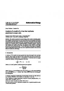
Application Example 1: A Complex Model for Influenza Infection Lee et al. Journal of Virology (2010): Airway/Lung Compartment d dt Ep d ∗ E p dt d dt V d dt D d ∗ D dt

= δE (E0 − Ep ) − βE Ep V, = βE Ep V − kE EP∗ TE (t) − δE ∗ Ep∗ , = πV Ep∗ − cV V − kV V A(t), = δD (D0 − D) − βD DV, = βD DV − δD∗ D∗ − γD∗ D∗

Ep : uninfected epithelial cells Ep∗ : infected epithelial cells V : free influenza virus D: immature dendritic cells D∗ : virus-loaded dendritic cells 16

Influenza Virus Infection Spleen/Lymph Node Compartment d dt DM d dt HN d dt HE d dt TN d dt TE d dt B d dt BA d dt Ps d dt PL d dt A

= kD D∗ (t − τD ) − δDM DM , = δHN (HN 0 − HN ) − πH (DM )HN , = πH (DM )HN + ρHE (DM )HE − δHE (DM )HE , = δTN (TN 0 − TN ) − πT (DM )TN , = πT (DM )TN + ρTE (DM )TE − δTE (DM )TE , = δB (B0 − B) − πB (DM )B,

= πB (DM )B + ρBA (DM + hHE )BA − δBA BA − πs BA − πL HE BA , = πs B A − δ s P s , = πL HE BA − δL PL , = πAS Ps + πAL PL − δA A 17

Two Compartment Flu Model Airway/Lung

(2)

(1)

(4)

(5)

Infected Epithelial cell (EP*)

Uninfected Epithelial cell (EP)

Immature dendritic cell (D)

Virus+ dendritic cell (D*)

(3)

Influenza virus (V)

(15)

Antiviral antibody (A)

(10)

Effector CD8 T cell (TE)

Long-lived Plasma cell (PL)

Naïve CD8 T cell (TN )

(14)

Short-lived Plasma cell (PS) (13)

(6)

(9)

(8)

Activated B cell (BA )

Naïve B cell (B)

(12)

(11)

Spleen/Lymph Node

18

Effector CD4 T cell (HE)

Mature Virus+ dendritic cell (DM )

(7)

Naïve CD4 T cell (HN )

19

Application Example 2: A Simplified Model for Influenza Infection • Use biological knowledge to de-couple or simplify the complex models • Design experiments to collect enough data • Fit the data to the models • Application of established models: biological interpretation, simulations, predictions and designing future experiments

20

Model Simplification Lung Compartment Model: Model Simplification Days 5-14 with adaptive immune response: decoupled the model d E dt p d ∗ E dt p d V dt

= ρE Ep − βa Ep V, = βa Ep V − δE ∗ Ep∗ − kE EP∗ TE (t), = Na Ep∗ − cV V − kV V A(t),

• V (t), TE (t) and A(t): measured • ((Ep (0), V (0), ρE , βa , δE ∗ , cV , kE , kV ): to be estimated • η(t) = cV + kV A(t): a time-varying parameter • Identifiability analysis: Need to fix Na 21

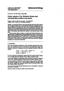
9 8

6 5 4 3 2 1 0 2

4

6

8

10

12

Days

Figure 1. Viral titer data (2007).

10000 20000 30000 40000 50000 60000 70000

Lung CD8 Smoothed by Cubic Spline

0

0

(CD8_2007$allcyto)

Viral Titer (log10)

7

0

20

40

60

80

CD8_2007$mydpi

Figure 2. Smoothed any positive CD8 data (2007).

22

14

16

500 0

(IGG2007$indIGG)

1000

IGG Smoothed by Cubic Spline

0

20

40

60

80

IGG2007$mydpi

300 200 0

100

(IGM2007$indIGM)

400

500

IGM Smoothed by Cubic Spline

0

20

40

60

80

IGM2007$mydpi

Figure 3. Smoothed IgG and IgM data (2007).

23

(a).

(b).

(c).

!

!

!

=1 EID50·ml-1·day-1·cell-1;

= 100 EID50·ml-1·day-1·cell-1;

= 1000 EID50·ml-1·day-1·cell-1;

Figure 1. Model fitting results for different virus production rate 24

Table 1. Estimation results with 95% bootstrap confidence intervals !

EID50· ml-1· day1 ·cell-1 1

100

1000

EP(0) cells per lung 2.3E+07 6.1E+06, 1.0E+09 2.4E+05 6.4E+04, 10E+06 2.3E+04 6.1E+03, 1.0E+06

E -1

day

9.9E-04 4.5E-06, 1.0 8.6E-04 4.8E-06, 1.00 9.2E-04 4.0E-06, 1.0E+00

! ml· EID501 day-1

kE cell-1 day-1

day-1

5.1E-06 8.5E-07, 1.8E-05 5.1E-06 9.1E-07, 1.7E-05 5.1E-06 8.9E-07, 1.8E-05

1.4E-05 3.7E10, 4.9E-05 1.4E-05 1.1E-10, 5.0E-05 1.4E-05 2.4E-10, 4.9E-05

1.2E+00 7.5E-01, 1.6E+00 1.2E+00 7.4E-01, 1.6E+00 1.2E+00 7.5E-01, 1.6E+00

25

E

*

kvG ml/ (pg !"#$

kvM ml/ (pg !"#$

3.1E-05 1.7E-08 1.6E-06, 4.4E-09, 5.2E-01) 7.0E-06 5.5E-06 4.5E-08 2.2E-06, 4.7E-09, 5.3E-01 8.1E-06 5.2E-06 2.6E-08 1.7E-06, 6.2E-09, 5.3E-01 8.4E-06

7.8E-02 5.2E-02, 8.1E+00 7.8E-02 5.1E-02, 8.1E+00 7.8E-02 5.1E-02, 8.2E+00

cv day-1

Table 2. Model selection results using AICc Model Full model E=0 kE=0, E =0 cv=0, kvG=0 cv=0, kvG=0, kvM =0 kvG=0 E=0, cv=0, *

26

RSS 49.4 49.4 360 49.4 484 49.4

AICc -33.2 -34.2 137 -36.2 159 -39.2

Figure 2. Comparison of the patterns of the estimated time-varying t ! , kVM AM (t ) and kVG AG (t ) parameter 27

(a)

(b)

(c)

(d)

(e)

(f)

Figure 3. The effects of different parameters on the peak viral load. (a) The effect of ! ; (b) The effect28of k E ; (c) The effect of E ; (d) The effect of kVM ; (e) The effect of ! ; (f) The effect of E p " 0 # *

Model Fitting Conclusions • We can reliably estimate the immune response kinetic parameters during the adaptive immune response period (Days 5-14): – The net growth rate of uninfected cells=the proliferation rate−the death rate: ρ = 0.339/day, larger compared to that during the first 5 days – The infection of epithelial cells: no targets – CTL effect: shorten the half-life of infected cells from 1.16 days to 0.59 days in average – IgM antibody effect: shorten the half-life of virus from 4 hours to 1.7 minutes in average.

29

Example 3: CD8+ T cell trafficking in mice with influenza infection Model structure identification d dt Tm d dt Ts d dt Tl

= [ρm Dm (t − τ ) − δm ]Tm − (γms + γml )Tm , = [ρs Ds (t − τ ) − δs ]Ts − γsl Ts + γms Tm , = γml Tm + γsl Ts − δl Tl ,

• Tm (t): CD8+ T cells in MLN • Ts (t): CD8+ T cells in Spleen • Tl (t): CD8+ T cells in Lung • Dm (t − τ ): DC cells in MLN with a time delay • Ds (t − τ ): DC cells in Spleen with a time delay

30

(3)

31

Example 3: CD8+ T cell trafficking in mice with influenza infection Hypothesis: Is the loss rate of CD8+ T cells in the lung δl =constant? d T dt m d T dt s d T dt l

= [ρm Dm (t − τ ) − δm ]Tm − (γms + γml )Tm , = [ρs Ds (t − τ ) − δs ]Ts − γsl Ts + γms Tm , = γml Tm + γsl Ts − δl (t)Tl , (4)

32

Example 3: CD8+ T cell trafficking in mice with influenza infection Hypothesis: Is there influx of CD8+ T cells from other tissues to spleen? d T dt m d T dt s d T dt l

= [ρm Dm (t − τ ) − δm ]Tm − (γms + γml )Tm , = [ρs Ds (t − τ ) − δs ]Ts − γsl Ts + γms Tm + ηs (t), = γml Tm + γsl Ts − δl (t)Tl , (5)

33

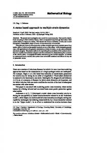
Example 4: Dynamic Gene Regulatory Network High-dimensional ODE models for dynamic gene regulatory network (GRN): p ∑ dxi = θij xj , i = 1, · · · , p, (6) dt j=1 where parameters Θ = {θij }i,j=1,··· ,p : quantify the interactions/regulations among the genes in the network. • Model selection: determine significant gene-gene interactions/regulations • ODE parameter estimation: quantify the strength of interacitons/regulations • Deal with high-dimensional and high computational cost 37

Dynamic GRN for Yeast Cell Cycle • Clustering 800 genes into 41 functional modules • High dimensional ODEs coupled with mixed-effects modeling techniques • A two-step smoothing approach coupled with the SCAD technique

39

15

10

15

15

5

10

15

Module 6 0.2

0.5 −1.0

5

10

Module 5

−1.5 0.0 1.5

Module 4

5

−0.6

10

−1.0

−0.6 0.0

0.5 −0.5

5

Module 3

1.0 2.5

Module 2 0.6

Module 1

5

15

5

Module 8*

10

15

Module 9*

5

10

15

−2

−2

−1.0

0

0.5

0 1

2

Module 7

10

5

15

15

0.4 5

10

15

5

Module 14*

10

15

Module 15*

−2

−0.6

−1

0

1

2

Module 13 0.2

15

Module 12

−0.6 10

10

−0.4

0.5 −0.5

5

5

Module 11 0.2 0.8

Module 10

10

5

10

15

5

15

5

Module 17

10

15

Module 18*

10

15

0 5

10

5

15

10

15

Module 21 0.5

0.5 −0.5

5

15

Module 20* −1.5 0.0 1.5

Module 19

10

−1.0

5

−2

−1.0

−0.6 0.0

0.5

2

Module 16

10

40 5

10

15

5

10

15

12 17

6

31

3 7

37

1

21

39 34

15

33

11 18

29

10

30 25

14

35

13 41 9

23 5

32

38

8 16

24

20 19 27

22 36

40

26 2

4 28

41

Example 5: Multi-Level Experiments for Influenza Infection • Mice with TIV or LAIV vaccination: blood, lung, spleen, LN and bone marrow samples • Humans with TIV or LAIV vaccination: blood samples, nasal washes (LAIV) • Frequent time course data: 13 time points • Multi-level data – Cellular level: flow cytometry, Elispot etc. – Protein/molecular level: Luminex – Genetic level: microarray

42

Multi-Scale and Multi-Type Models • Multi-scale and multi-level models – Genetics level: time course microarray data – Protein level: cytokines and chemokines – Cellular level: flow cytometry data – Multi-level integration • Multi-type models: ODE, SDE, state-space models, stochastic process models, agent-based models, network models • Multi-scale and multi-type model integration

43

Summary: Multi-Level, Multi-Scale and Multi-Compartment Models

44

Software Tools • Develop more efficient computational algorithms for model simulations and parameter estimation • Develop user-friendly software tools for modeling, simulation and estimation • Develop web-based data management tools for high-throughput biomedical data

45

DEDiscover 2.0 Differential Equation Modeling Software

Center for Biodefense Immune Modeling

DEDiscover is a software tool for developing, exploring, and applying differential equation models. It provides simulation, prediction, and parameter estimation (data fitting) facilities for systems of ordinary and delayed differential equations, and includes a set of example models for infectious diseases. Free Download: http://cbim.urmc.rochester.edu/software/dediscover

46

47

Summary: Biomedical Research System Biomedical Research

Experiments

Data Management

Quantitative Sciences

Statistical Analysis

Software Development

Math Modeling

Computing

Computing Hardware & Admin 48

Challenges and Discussions • Integrating quantitative sciences into a new interdisciplinary field – Biomathematics – Bioengineering and biophysics – Bioinformatics and Biocomputing – Biostatistics • Quantitative Sciences: important and a strong impact to – Life sciences and biomedical research – Clinical practice and public health – Experimental systems biology approach • Interdisciplinary Quantitative Sciences: Challenges – Lack of strong interdisciplinary leaders – Long-term visions – Lack of collaboration, communication and coordination for the investigators from different disciplines 49

Acknowledgement Immunologists: Zand, Welle Topham, Mosmann, Ward, Jin

Experiments (Lab Postdocs & Technicians)

Data Management: Holden-Wiltse Zhang, Yang, Massaro

Quantitative Sciences Hulin Wu

Statistical Analysis: Liang Xue, Kumar, Lu, Wu, Yang

Software Development: Stover, Warnes, Ma, LeBlanc, Crowley, Wu, William,

Math Modeling: Miao Perelson, Mugwagwa

Computing: Warnes, Miao

Computing Hardware & Admin: IT Staff 51

Acknowledgments • NIAID/NIH grant R01 AI 055290: AIDS Clinical Trial Modeling and Simulations • NIAID/NIH grant N01 AI50020: Center for Biodefense Immune Modeling • NIAID/NIH grant P30 AI078498: Developmental Center for AIDS Research • NIAID/NIH grant R21 AI078842: Analysis of Differential Resistance Emergence Risk for Differential Treatment Applications • NIAID/NIH grant RO1 AI087135: Estimation Methods for Nonlinear ODE Models in AIDS Research 52