IOP Conference Series: Materials Science and Engineering
PAPER • OPEN ACCESS
Development of modelling algorithm of technological systems by statistical tests To cite this article: E A Shemshura et al 2018 IOP Conf. Ser.: Mater. Sci. Eng. 327 042072
View the article online for updates and enhancements.
This content was downloaded from IP address 179.61.154.171 on 12/04/2018 at 13:40
MEACS 2017 IOP Publishing IOP Conf. Series: Materials Science and Engineering 327 (2018) 042072 doi:10.1088/1757-899X/327/4/042072 1234567890‘’“”
Development of modelling algorithm of technological systems by statistical tests E A Shemshura, A V Otrokov and V G Chernyh Shakhty Institute of Platov South-Russian State Polytechnic University (NPI), Lenin Sq., Shakhty, Rostov Region, 646500, Russia E-mail:
[email protected] Abstract. The paper tackles the problem of economic assessment of design efficiency regarding various technological systems at the stage of their operation. The modelling algorithm of a technological system was performed using statistical tests and with account of the reliability index allows estimating the level of machinery technical excellence and defining the efficiency of design reliability against its performance. Economic feasibility of its application shall be determined on the basis of service quality of a technological system with further forecasting of volumes and the range of spare parts supply.
1. Introduction At present, it is critical to make a sound choice of technological systems ensuring the minimum operation cost until their write-off thus complying with all required restrictions on productivity and performance standards of the equipment [1-3]. One of the possible ways to solve this task is to develop modelling algorithms that would provide for the simulation of technological systems [4-6]. The technological system is understood as the set of equipment, machines, and units associated with each other and operating to produce a useful effect in any production. Simulation modelling of technological systems represents a numerical experimental method and considers the influence of random factors on system behavior during the generated time. The modelling shall result in the numerical value of an accepted system performance evaluation criterion, i.e. minimum operation costs. 2. Cost model of technological system In order to assess the design efficiency of any equipment within a machine system, the mathematical model was developed with account of its operating costs, thus connecting technological system performance with its cost. ∙ ∑
.
∙
∙
'… ∑* )
∙
) %
.
#∙
∙ %
.
#
∙!∙"
+
∙∑
∙ ∑
,
∙-.
#
∙
∙
∙/∙+ #. 0
∑
#. $% ∙
# 123
#.
%$⋯'
(1)
where n – number of subsystems; Сb – subsystem net book value; Тres.Σ – subsystem life before writeoff; Q – technological system performance; Кss – stock and inventory costs ratio; τdr – operator’s Content from this work may be used under the terms of the Creative Commons Attribution 3.0 licence. Any further distribution of this work must maintain attribution to the author(s) and the title of the work, journal citation and DOI. Published under licence by IOP Publishing Ltd 1
MEACS 2017 IOP Publishing IOP Conf. Series: Materials Science and Engineering 327 (2018) 042072 doi:10.1088/1757-899X/327/4/042072 1234567890‘’“”
payment rate; tsh – shift duration; Тsw – total workload of support services per shift; z – energy rate; NΣ – total subsystem electric power per job; Кss – average power demand ratio within shift; t – relative subsystem runtime per shift; К – subsystem overhaul cost; Тrep – average overhaul time; Тres – current subsystem lifetime; α – costs of subsystem dismantling, transportation and mounting per every overhaul; Тrep.exm, Тmin.rep – subsystem meantime between repairs and maintenance respectively; l – number of repairs; Сrep.exm, Сmin.rep – costs of repairs and servicing respectively (2), (3); Тrep.sub – subsystem average fault correction time; m – maintenance manpower. С567.68/ = :5; ∙ / ; >/
[email protected] = :5; ∙ 57 + >/ ,
(2) (3)
where τrw – average hourly salary of maintenance staff; qrep.exm, qmin.rep – labor intensity of repairs and maintenance respectively; Сrp, Сm – costs of spare parts and consumables respectively; λ – subsystem failure rate. The suggested expression (1) allows defining the given costs of technological system performance at any moment and assessing technological performance of machines, efficiency of their modernization, economic feasibility of their application. 3. Simulation modelling algorithm Below is the sequence of simulation modelling measures taking into account logical and probabilistic approach and principles of statistical tests (Monte Carlo method) [7, 8]: - to define construction and functional schemes of a technological system and its machinery; - to explain and create the reliability model; - to adopt regulations on time between failures and recovery time for every functional machine or unit and set parameters taking into account specific operating conditions; - to design the modelling algorithm depending on the mission: task 1 – comparative performance analysis of repairable machines; task 2 – integral estimation of machine reliability; task 3 – determination of optimal term of machine runtime (optimization task); - to set time between repairs and machine runtime before write-off. Pretest reliability analysis may form the basis for mathematical representation of machine operation [9, 10]. In this case the design object represents a complex technical system, in particular, a single-function unit, intended to perform a certain task and consisting of some functional elements. The operation of such system represents the sequence of various states of its elements: - workable – fitness for purpose, partial failure; - unworkable – complete failure. Each element lies within one of two states: A? B = C
1 FG F-Bℎ IJIKILB FM NOPQRSJI; ' 0 FG F-Bℎ IJIKILB FM VLNOPQRSJI.
(4)
The system state is described by the state vector of system elements: X A , AZ , … , A@ ∈ 2@ , W
(5)
X B + bB c ]^,_ B = PaW
(6)
where n – number of system elements. It is considered that the system state change is described by homogeneous Markov process with continuous time and finite discrete states i, which is characterized by stationary transfer of the rate matrix from state i into state j:
2
MEACS 2017 IOP Publishing IOP Conf. Series: Materials Science and Engineering 327 (2018) 042072 doi:10.1088/1757-899X/327/4/042072 1234567890‘’“”
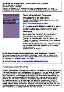
Possible system states and transitions between them are presented as a marked state graph. Fig. 1 shows the system state graph consisting of two elements. Each element of the system is characterized by constant failure rate λi and constant recovery rate μi. Values λidt and μidt represent the system transition rate from one state into another within time interval dt.
Figure 1. Marked state graph Probabilities of states are used to describe a random process taking place within this system, and thus the following system of Kolmogorov equations is established: ]hi B ]i BB i f ]Z BB e ]ji BB g
= l m + mZ · ]h B = n · ] B = nZ · ]Z B 9 m · ]h B = nZ · ]j B l n" = mZ · ] B ' 9 mZ · ]h B = n · ]o B l n" = m · ]Z B 9 m · ]Z B = mZ · ] B l n = n" · ]j B
(7)
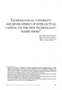
Probabilities of a system in either state within some time t for the suggested state graph are defined proceeding from initial conditions and random values distribution law regarding workable state failures and recovery rates. Systems consisting of more elements can be presented in a similar way. A software program was designed to describe the above-mentioned behavior. behavior The program includes the following steps: - failure-free time of certain subsystems within the technological system is generated according to the established distribution laws (example is given in Fig. 2); - first failed subsystem or unit is defined on the basis of state probability of different units and according to formula (7), then this time between failures is summarized with the total operating time of a technological system; а)
b)
Figure 2. Generator (а) and histogram (b) of time between failures distribution - downtime of a failed unit is generated according to the established recovery time laws; - current assessment of reliability indicators of a failed unit and the technological system in general, as well as the assessment of system unit cost is made;
3
MEACS 2017 IOP Publishing IOP Conf. Series: Materials Science and Engineering 327 (2018) 042072 doi:10.1088/1757-899X/327/4/042072 1234567890‘’“”
- performance of a technological system within time in operation and current unit operating cost of a system (1) is calculated; - new operating time is generated by a corresponding random value generator and residual failurefailure free operating time is defined for a failed unit. unit All this demonstrates the modelling mode of a technological system through random values with established distribution laws for the generation of failure-free operating time and recovery time of subsystems. 4. Simulation modelling results The above-mentioned algorithm is implemented in Mathcad, which was used for simulation modelling of a technological system representing a set of mining machines for underground construction and tunneling. As a result, the modelling is provided for qualitative and quantitative evaluation of the designed algorithm for tunneling machines. machines Qualitative evaluation is made proceeding from the general logic of operation with regard to considered technological systems. Quantitative evaluation is made through comparison of numerical results of modelling model with performance indicators of a technological system in similar operating conditions. The example of modelling (Fig Fig. 3, a) shows that the operating cost of subsystems decreases over time in general; however this is accompanied by a sharp cost increase in case of overhauls or expensive maintenance. It is also possible to compare two and more technological systems (Fig. ( 3, b) throughout their entire operating time, which allows for more weighed estimate unlike separate operating criteria. a)
b)
Figure 3. Unit cost (a) and comparison (b) of technological systems 5. Conclusions The designed algorithms and the software program allow defining the given operating costs of technological systems taking into account random failures and recovery rates at any time of failure. Minor updates of modelling ling algorithm make it possible to solve additional tasks, i.e. comparative analysis of technological systems, integrated estimate of system performance, performance and definition of optimal terms of technological subsystem failures. If applied in industry, the above-mentioned above algorithm will ensure reliability and validity of decisionss with regard to production equipment and will reduce operating costs by 10-12%. References [1] Nosenko A S, Domnitskiy A A and Shemshura E A 2017 Predictive reliability assessment of loading and transport modules of tunneling equipment during construction of road tunnels. tunnels Procedia Engineering. 206 61-66 [2] Jonge B, Dijkstra A S and Romeijnders W 2015 Cost benefits of postponing time-based time maintenance under lifetime distribution uncertainty. uncertainty Reliability Engineering & System Safety. Safety 4
MEACS 2017 IOP Publishing IOP Conf. Series: Materials Science and Engineering 327 (2018) 042072 doi:10.1088/1757-899X/327/4/042072 1234567890‘’“”
140 15-21 Zhang W and Wang W 2014 Cost modelling in maintenance strategy optimization for infrastructure assets with limited data. Reliability Engineering & System Safety 130 33-41 [4] Otrokov A V 2002 Computer-aided synthesis of technical solutions for mine loading machines. Izvestiya Vysshikh Uchebnykh Zavedenii. Gornyi Zhurnal. 5 27-30 [5] Doronin S V and Moskvichev V V, 2007 Simulating strength, reliability, and viability for damaged structural elements. Chemical and Petroleum Engineering. 43 (1-2) 51-59 [6] Uthman Said and Sharareh Taghip 2017 Modeling failure process and quantifying the effects of multiple types of preventive maintenance for a repairable system. Quality and Reliability Engineering international. 33 (5) 49-61 [7] Shaimardanov L G and Boiko O G, 2016 Use of the Monte Carlo method for simulating the process of change in failure-free operation of repairable systems. J. Mach. Manuf. Reliab. 45 (1) 90-94 [8] Windebank E A 1983 Monte Carlo simulation method versus a general analytical method for determining reliability measures of repairable systems. Reliability Engineering. 5 (2) 73-81 [9] Wu X and Hillston J 2015 Mission reliability of semi-Markov systems under generalized operational time requirements. Reliability Engineering & System Safety. 140 122-129 [10] Javier Faulin, Angel A. Juan, Carles Serrat, Vicente Bargueño 2008 Predicting availability functions in time-dependent complex systems with SAEDES simulation algorithms. Reliability Engineering & System Safety 93 (11) 61-71
[3]
5