Development of Online Tools to Support GIS Watershed Analysis. W. Elliot. July, 2016. In 1996, the Stream Team organized a meeting of hydrologists from every ...
Development of Online Tools to Support GIS Watershed Analysis W. Elliot July, 2016 In 1996, the Stream Team organized a meeting of hydrologists from every Forest Service Region and Forest Service Scientists engaged in watershed-related research to a meeting in Tucson. The focus of the meeting was to identify tools that needed to be developed to support watershed management. One of the tools that was suggested was a GIS-based tool that could run on the internet. At that time, Federal web sites were in their infancy, and the development of GIS tools for watershed analysis was only just beginning. Scientists at the Forest Service Rocky Mountain Research Station (RMRS) took this challenge to heart. In 1999, with support from the San Dimas Technology and Development Center, they introduced the first ever online interface to the Water Erosion Prediction Project (WEPP) model to predict soil erosion for forest road segments and forest hillslopes disturbed by wildfire and forest management (http://forest.moscowfsl.wsu.edu/fswepp/ )These interfaces were very quickly adapted by the Forest Service and other land management agencies. About 2000, a GIS interface was developed by the USDA Agricultural Research Service (ARS) National Soil Erosion Research Laboratory for the WEPP Watershed Version. The interface ran in ArcView, and shortly after introducing it, a GIS wizard was developed to aid in applying GIS tools to predict erosion from hillslope polygons delineated by the wizard using the WEPP model. Two grants were received from the Joint Fire Science Program to further enhance this tool, known as GeoWEPP, for Forest Conditions. It was upgraded to run in ArcMap 8.x and continues to be upgraded for current versions of ArcMap by the State University of New York, Buffalo. When field personnel tried to apply this tool, however, they soon found that they did not have the time to develop the level of GIS skills required to use GeoWEPP. In the early 2000s, the ARS also developed a proof of concept online GIS watershed tool that was not intended for widespread application. In 2009, the Army Corps of Engineers, Chicago Office, approached RMRS to develop an online sediment delivery tool that could be applied to forested watersheds in the Great Lakes Basin. RMRS, in collaboration with the ARS and Washington State University collaborated to develop a user friendly online GIS tool that could be used to support forest watershed management. The team built on the prototype tool from 10 years earlier, and upgraded it with a Google Map interface to zoom into sites. A comprehensive forest soil and management database similar to the FSWEPP database was added. The interface accessed digital elevation data from a USGS server, and an 800-m climate database from the Natural Resource Conservation Service (NRCS). The interface also accesses the USGS land cover database and NRCS SSRUGO Soils Database. For a single run, the watershed area is limited at the moment to about 400 ha (1,000 acres). On larger watersheds, spatial variability of weather becomes important, with higher elevations of the watershed receiving more precipitation, and much of that as snow. Work is ongoing to incorporate climate variability into the model and increase the area that can be modeled. The level of skill necessary to use the model is similar to that required to use other online mapping tools with advanced features, such as Google Earth. An online set of instructions can be downloaded to guide the use through the steps necessary to carry out a post wildfire run, or a set of fuel management runs. Figure 1 summarizes the four recommended runs (Low severity wildfire; Thinning, Prescribed Fire,
Forested). The example in Figure 1 is from the East Deer Creek watershed in the Colville National Forest, a watershed that provides water to a nearby town. To use this tool, the user first zooms to a site of interest, builds a channel network, and selects an outlet point for the sub watershed of interest (Figure 1a). This sub watershed is then run for the four scenarios. The results of each run can be saved as maps and tables, and allow the user to compare the potential sediment delivery from forest management to that from an undisturbed forest and a wildfire. Figure 1 shows some of the results from the four runs. Figure 1.f shows the distribution of predicted surface runoff plus lateral flow following a prescribed burn. Note that not all hillslopes respond the same way to a prescribed burn. The maps shown in Figure 1.b – 1.e are useful in helping managers decide which hillslopes may be at risk to the greatest erosion, and prioritize those hillslopes for treatment. The example analysis shows that the hillslope at the top of the watershed has the greatest erosion risk, so managers may consider practices other than prescribed fire to treat this slope, like thinning followed by mastication, or doing a prescribed burn in early summer when conditions are damp, and the loss of duff will be minimal when burning slash or understory. Users can export the results of each run for importing into ArcMap, where the results from several runs can be displayed in a single map. A recommended approach for summarizing the model outputs is outlined in Table 1. With this approach, the sediment delivery associated with the disturbance is divided by the frequency of the disturbance to determine an average annual sediment delivery associated with the disturbance. In the example in Table 1, this average is less than the annual sediment delivery from an undisturbed forest, suggesting that in the long term, sediment delivery on this watershed is not impacted by disturbance. Table 1 also shows the estimated sediment delivery the year of the disturbance, which may be of interest to downstream water users in that year. The interface can also predict return period values for daily sediment delivery, a number that can be considered a reasonable estimate for a Total Maximum Daily Load. Figure 1.b – 1.e also shows the predicted peak flow rates at the outlet of this watershed, which is at a road-stream crossing. Note that the estimated post wildfire peak flow is nearly 20 times greater than the peak flow for an undisturbed forest. The online documentation shows how to carry out an analysis where not all hillslopes are treated the same in a given year. A complimentary online interface to be used after wildfire is under development (http://129.101.152.143/baer/). It can currently predict the erosion following a wildfire, and work is ongoing to allow users to compare this to prefire conditions and to evaluate the benefits of mulching. Another interface is under development for the Lake Tahoe Basin that is incorporating enhanced output analyses to predict delivery of phosphorus and fine sediment (silt- and clay-size particles and aggregates). Once complete, it can be applied nation-wide. A prototype interface is under development for predicting sediment delivery from roads within a watershed. Because the national road database is so large, further resources will be needed to develop a consistent road database to support it. The road interface has been used once to support an analysis in a sensitive area within the Colville National Forest. A similar interface was also developed for post mining conditions where a user could upload a post mining digital elevation model, but the interface is not currently online. It included advanced features to aid users in evaluating the effectiveness of sediment basins. Post mining landscapes tend to be less steep, and less susceptible to soil erosion. Were there sufficient interest, the post mining interface could also be reactiviated.
Figure 1. Example of a set of runs on an online interface. The watershed area was limited to only 32 ha (80 a) for this example, located in the Colville National Forest. The interfaces determined that the watershed was 96 percent forest. The erosion rates shown are for estimated hillslope erosion.
a. Delineated Sub watersheds
b. Wildfire Erosion; Pink is greater than 1 Mg/ha, Green is less than 1 Mg/ha; 10-y Peak Flow is 8.8 m3/s
c. Thinning; Light green is less than 0.1 Mg/ha, Dark green is less than .025 Mg/ha; 10-y Peak Flow is 5.3 m3/s
d. Prescribed Fire; Light green is less than 0.1 Mg/ha, Dark green is less than .025 Mg/ha 10-y Peak Flow is 5.3 m3/s
e. Undisturbed Forest; Predicted hillslope erosion is 0; 10-y Peak Flow is 0.47 m3/s
f. Prescribed Fire: Surface runoff and lateral flow. Dark polygon is 150 mm/y, lighter polygon is 120 mm/y and lightest polygon is 105 mm/y.
Table 1. Summary of fuel management analysis. Column 2 is the average predicted erosion for the eyar following the disturbance; average annual sediment delivery is the erosion rate following the disturbance divided by the frequency of the disturbance. In this watershed, erosion rates from wildfire, prescribed fire, and thinning are all sufficiently low that when averaged over the frequency of the disturbance, they are unlikely to change the long term average sediment yield. This analysis assumes all hillslopes are treated the same. Unmanaged Land Use Disturbance Disturbed Frequency Erosion (y) (Mg ha-1) Forest Wildfire
1 40
Weighted Average
0.1 0.8
Avg Annual Erosion (Mg ha-1) 0.1