Application Specific Integrated Circuit (ASIC) design, has made possible the development of ..... data fluctuates randomly about a true value representing a noise free signal. This is due to noise effects ...... Description: Add source operand S to the destination operand D and store the result in ...... 1. HY =XY. ____________I.
III ONR Grant No. N00014-91-J-1011 R&T Project: 4148501---02
AD-A253 680 Semi-Annual Report
1
DEVELOPMENT OF PARALLEL ARCHITECTURES FOR SENSOR ARRAY PROCESSING ALGORITHMS
I
D T IC fIl ......SELECT JUL311992
Submittedto: Department of the Navy Office of the Chief of the Naval Research Arlington, VA 22217-5000
I
Submitted by:. M. M. Jamali Principal Investigator
U
S. C. Kwatra Co-Investigator
Ih~ I
docoiment has been approved
forpublic release and sole; its distzibufion is unlimited-
Department of Electrical Engineering College of Engineering
The University of Toledo Ohio 43606 IToledo, Report No. DSPH-2
5
July 1992
92-19258
LI
U I
I
3
3 *Parallel
ABSTRACT The high resolution direction-of-arrival (DOA) estimation has been an important area of research for number of years. Many researchers have developed number of algorithms in this area. Fast advancement in the areas of Very Large Scale Integration (VLSI), Computer Aided Design (CAD) and Application Specific Integrated Circuit (ASIC) design, has made possible the development of dedicated hardware for sensor array processing algorithms. In this research we have first focussed our research for the development of parallel architecture for Multiple Signal Classification (MUSIC) and Estimation of Signal Parameter via Rotational Invariance Technique (ESPRIT) algorithms for the narrow band sources. The second part of this research is to perform DOA estimation for the wideband sources using two algorithms. All these algorithms have been substituted with computationally efficient modules and converted them to pipelined and parallel algorithms. Architectures for the computation of these algorithms and architectures has been developed. Simulations of these algorithms and
5architectures
has been performed and more detailed simulations are in
progress.
I
U
3
Chapter 1 presents theoretical and mathematical aspect of MUSIC/ ESPRIT algorithms. These algorithms are modified and parallelized for narrow band case in chapter 2. Hardware implementations of these algorithms are in Chapter 3. Development of Generalized Processor - GP is shown in Chapter 4. In Chapter 5 DOA estimation for Broad-Band sources using "Broad-Band Signal Subspace Spatial-Spectral" (BASS-ALE) Estimation algorithm and its architecture is described.
Chapter 6 gives the details of
hardware development for the bilinear transformation approach for wide band sources. Data generation and simulation of DOA estimation both for narrow band and wideband cases are given in Chapter 7. Conclusions and
future directions are described in Chapter 8.
Accesion For NTIS Ui i UJ,.
Statement A per telecon Clifford Lau ONR/Code 1114
Arlington, VA
CRA& TAB T
L1
,w:o-., :ted
[]
J.A,;cdlion By........
NWW 7/30/92
pyre
Mv,,b~gy Cc~r
QUALITY INSPECTED Z
r'i0 Va ' !
Di -t
t
Jl . ;
.
Of
I I Table of Contents SABSTRACT
i
LIST OF FIGURES
I
Chapter 1
3
£
£
v
2
Introduction to array signal processing Introduction
1
Data model
3
MUSIC algorithm
8
ESPRIT algorithm
13
TLS ESPRIT algorithm
16
Improved TLS ESPRIT algorithm
19
Eigendecomposition using Householders transformation and given's rotation
I 3
1
3
23
Symmetrical eigendecomposition problem
23
Non symmetrical eigendecomposition problem
38
Parallel architecture for MUSIC algorithm
43
Introduction
43
Literature search
44
Hardware block diagram of MUSIC and ESPRIT algorithms
3 4
I
1
45
Data covariance matrix formation
45
Hardware for Householders transformations
50
Parallel algorithm for tridiagonal QR algorithm
52
Hardware implementation of power method
63
Conclusions
63
Development of architecture for MUSIC algorithm and
i
I I generalized processing elements
3 i
3
5
Pipelined stages and buffers in MUSIC algorithm
69
The generalized processor
71
Instruction set details
75
Programming details
79
DOA estimation for broad-band sources using "Broad-Band Signal-Subspace Spatial (BASS-ALE) estimation" algorithm Introduction
I
69
88 88
"Coherent signal-subspace processing for detection and estimation of angles of arrival of multiple wide-band
3 3 5
sources"
88
Architecture for "Broad-band signal-subspace spatial-spectral (BASS-ALE) estimation" algorithm
90
Signal and noise-only subspaces
92
Spatial/ temporal noise decorrelating
93
Basic BASS-ALE estimator
93
Broad-band covariance matrix estimation
94
Signal-subspace order estimation
94
Architecture for BASS-ALE algorithm
97
Broad-band covariance matrix estimation architecture
5 3
using 64 processing elements
98
Broad-band covariance matrix estimation architecture using 64 processing elements (an overlapped approach)
101
Broad-band covariance matrix estimation architecture using eight processing elements
106
I
Hardware design
108
i
Conclusions
116
iii
I 3
6
DOA estimation for broadband sources using a bilinear transformation matrix approach
3 i
3 I I
7
8
APPENDIX
I I
118
Problem formulation
119
Problem solution
121
Parallelization and modification
124
Computation of transformation matrices
128
Computation of G
130
Cholesky decomposition
131
Hardware implementation
135
Covariance matrix computation
138
Computation of G
142
Computation of Gn
147
Forward substitution
147
Cholesky decomposition
149
Conclusions
152 154
Data generation and simulation for narrow band signals
154
Simulation results for broad-band signals
167
Conclusions
i
1
Introduction
Computer Simulation
3
118
170
Work performed
170
Future work
172
REFERENCES
i iv
I I U
LIST OF FIGURES
Figure
1 3
1.1
A two sensor array
1.2
Typical array scene
1.3
Signal subspace & array manifold for a two-source example
1.4
Sensor array for ESPRIT
3.1
Hardware block diagram for MUSIC
3.2
Hardware block diagram for ESPRIT
3.3
Architecture for the computation of covariance matrix
3.4
Architecture for Householders transformation
3.5
Updating eigenvalues
3.6(a)
Updating eigenvectors during odd step
3.6(b)
Updating eigenvectors during even step
3.7
Hardware for power method
4.1
Various stages and buffers in MUSIC algorithm
4.2
Architecture for Generalized Processor GP
5.1
Procedural diagram showing different units involved in BASS-ALE
*
estimation 5.2
I1
3
Product of 64-element vector x by its conjugate transpose resulting in lower triangular matrix
5.3
Architecture to produce a lower diagonal matrix without superimposed columns
5.4
1 3
I
Product of 64-element vector x by its conjugate transpose resulting in lower triangular matrix where its columns overlap
5.5
Architecture to produce a lower diagonal matrix with superimposed columns
V
I 3
5.6
Flowchart of data from the delay array to the 64 PE multiplication unit
5.7
Vector multiplication
5.8
Block diagram overview of 8 PE architecture to compute lower diagonal
5.9
Flowchart illustrating the use of 3 counters to multiply 36 sub matrices
*matrix
5
forming a lower triangular matrix 5.10
Detailed floor plan of 8 PE architecture to produce a lower triangular matrix
3
3 3 3
5.11
Dual port RAM control block
5.12
Detailed internal structure of a PE
6.1
Flowchart for wideband algorithm
6.lb
Mathematical transformation in the algorithm
6.2
Flowchart of cholesky decomposition
6.3
Overall system architecture till computation of G
6.4
Architecture for the computation of Covariance matrix
6.5
Flowchart for the computation of covariance matrix
6.6
Processing Elements for covariance matrix
6.7
Flowchart to compute G matrix
6.8
Processing element for the computation of G matrix
6.9
Fully pipelined and parallel architecture for forward substitution
I
3 3 5 g I
method 6.10
Typical PE for forward substitution method
6.11
Architecture for cholesky decomposition
6.12
Processing element for cholesky decomposition
7.1
Inphase and quadrature component
7.2
Spatial specrtra without orthogonalization
7.3
Spatial specrtra with orthogonalization vi
7.4
Spatial specrtra without orthogonalization
7.5
Spatial specrtra with orthogonalization
7.6
M array with N delays
vii
Chapter 1
INTRODUCTION TO ARRAY SIGNAL PROCESSING
1.1 INTRODUCTION
The high resolution direction-of-arrival (DOA) estimation is important in many sensor systems.
It is based on the processing of the received signal and
extracting the desired parameters of the DOA of plane waves. Many approaches have been used for the purpose of implementing the function required for the DOA estimation including the so called maximum likelihood (ML) and the maximum entropy (ME) methods [1-3]. Although they are widely used, they have met with only moderate success.
The ML method yields to a set of highly non linear
equations, while the ME introduces bias and sensibility parameters estimates due to use of an incorrect mode (e.g. AR rather than ARMA).
The Multiple Signal
Classification (MUSIC) and the Estimation of Signal Parameters by Rotational Invariance techniques (ESPRIT) algorithms are two novel approaches used recently to provide asymptotically unbiased and efficient estimates of the DOA [4,5]. They are believed to be the most promising and leading candidates for further study and hardware implementation for real time applications. They estimate the so called signal subspace from the array measurements.
The parameters of interest (i.e.
determiaing of the DOA) are then estimated from the intersection between the array manifold and the estimated subspace.
An important aspect of the design of a signal processing system for the DOA is the computation of the spectral decomposition. In recent years, the search for useful algorithms and their associated architecture using special purpose processors
I I has been a challenging task. Such high performance processors are often required to be used in real time application; thus, it is felt that they should rely on efficient implementation of the algorithms by exploiting pipelining and parallel processing to achieve a high throughput rate. The QR algorithm is one of the most promising for the spectral decomposition problem due to its stability, convergence rate
3 g 3
I
properties, and suitability for VLSI implementation [61.
A number of investigations have been concerned with finding efficient algorithms to solve the spectral decomposition problem based on the QR algorithm. These investigations have mostly relied on systolic arrays approach. A primary reason for employing such approach is that it is believed to offer a well-motivated methodology for handling the high computation rate required for a real time
3 I
3
application.
A useful property of the QR transformations is that shifts can be used to
3
increase the rate of convergence to locate the eigenvalues [71. This may be very useful for some systems applications
where the computations of the eigenvalues
I
are sufficient, such as matrix rank determination and system identification. However, in other applications, (e.g. , direction of arrival estimation, spectral estimation, and antenna beamformation), the computation of both the eigenvectors
5
and eigenvalues is crucial [4-8], and one might use the QR algorithm without shifts to obtain these parameters in parallel. In such a case, this algorithm may require a sufficiently large number of iterations to converge. Keeping the number of iterations low may yield to inferior results such as in MUSIC and ESPRIT algorithms, where an accurate computation of the eigenvalues and eigenvectors will also determine the accuracy of the direction of arrival (DOA's)
.
3
For example,
23!
2
for the MUSIC algorithm [8], once we determine the signal and noise subspaces from the eignenvectors, the spacial spectra is determined by
S(O) =
H
I
H a (E)EN EN a(E)
(1.1)
where EN is the matrix of eigenvectors spanning the noise subspace, and a(0) = [1, exp(-j0), exp( -2je), ...
,
exp( -jE(m-1 )]
(1.2)
with m being the number of sensors, and H denoting complex conjugate transpose. Also , one drawback of the QR algorithm is that when applied to a dense matrix, it may be very time-consuming and may pose difficulties for parallel implementation due to communication and timing among different modules of the systolic array [ 9 1. For this reason, currently, there is no known simple efficient systolic array approach using the QR algorithm that is capable of generating the eigenvectors and eingenvalues in parallel.
1.2 DATA MODEL
For the purpose of understanding the advantages of using a sensor array in DOA estimation, it is necessary to explore the nature of signals and noise the array is desired to receive.
It is well known that in active sensing situations, the scattered
data fluctuates randomly about a true value representing a noise free signal. This is due to noise effects and errors in a sensor array system. These fluctuations can be both additive and multiplicative.
The additive fluctuations are due to thermal
noise, shot noise, atmospheric noise, and other kinds of noise which are independent of the desired signal.
The multiplicative fluctuations are due to
measured errors in estimating the signal amplitudes, gain variation, etc. A noise
3
model that represents all these noise effects is, in general, difficult to obtain, especially when some of the noise sources are dominant. Usually, based on the
n
noise models, additive and/or multiplicative, the calculated probability of error, as a function of the noise power, is practically similar in each case. This indicates that the noise power, rather than its specific characteristics, has more impact on the sensor array performance. Moreover, one is usually concerned with the effects of the additive noise on the output of a sensor array system. For this reason, an
I
additive noise would be appropriate to choose for the evaluation of the performance of a system. This noise represents the totality of small independent sources, and by
first narrow band signals are considered where it is assumed that the power of all
3 3
emitter signals is concentrated in the same narrow frequency band. In this context,
N
virtue of the central limit theorem one can model the resulting noise as Gaussian and (usually) stationary process. Also, to make the problem analytically tractable,
two more assumptions that are of interest are invoked. First, it is assumed that the sources are in the far field of the array, consequently the radiation impinging on the array is in the form of plane waves, and secondly, the transmission medium is assumed to be isot.ropic so that the radiation propagates in straight line. Basd on
1 5
these assumptions, the output of any array element can be represented by a time advanced version or time delayed version of the received signal at a reference element as shown in Figure 1.1. Since the narrow-band signals are assumed to have the same known frequency co, the received signals at the reference sensor and the second sensor are respectively
3 3
given by s(t) = u(t) exp[ j(wot + v(t))]
(1.3)
s(t-t) = u(t- 0 exp[ j(o 0o (t - T)+ v(t- T)M
(1.4)
3 I
.=,a n4 m R
nnnnmn
nno
3N~l
I I Is(t-
where u(t), and v(t) are the amplitude and phase of s(t) respectively. The signal -0at the second sensor is delayed by the time required for the plane wave to propagate through A sin 0,and if c represents the velocity of propagation, then this
Itime delay
T is given by
I
~A
Sn0
Plane wave
I
Reference element
Second sensor element
A
IFigure
1.1: A two sensor array
I
- A sin cin 0(15
(1.5)
C
I
The narrow band assumption implies that u(t) and v(t) are slowly varying functions, thus:
I
u(t)
=
u(t-)
v(t) = v(t-T)
I I I5
(1.6)
(1.7)
U I for all possible propagation delays. Thus the effect of a time delay on the received
I
signal is simply a phase shift: s(t-T)= s(t)exp(-jooT)
(1.8)
I
3 Now consider an array consisting of m sensors and receiving signals from d sources located at directions 01 02,
0 d with respect to the line of array, as shown in Figure 0..
1
1.2.
Sensors
I I Reference element
!
3
Figure 1.2: Typical array scene.
It is assumed that none of the signals are coherent. Using superposition of signal contribution, the received signal at the kth sensor can be written as
3 I
d
ak(0) S i(t-Tk(0
Xk(t)
) ) +
nk(t)
i=l
63I
d
ak(0 ) S i(t) exp(-jco o (0 ) ) + n k(t)
=
(1.9)
1=1
where
I
k(0 i) is the propagation delay between a reference point and the kth sensor
for the ith, wavefront impinging on the array from direction
0i, a k(O i) is the
corresponding sensor element complex response (gain and phase) at frequency co
, and
nk(t) stands for the additive noise at the kth sensor. If we let
a( 0 i) = { a 1(0 i)exp(jo 0oT I(Oi
)) .... a
m(0 i)exp(jw oT m(O i))}H
(1.10)
Where H denotes complex conjugate transpose n(t) = I n I(t), n 2(t .............. n m(t)}T and the data model representing the outputs of m sensors becomes d
x(t)=1a( 0 i)s i(t) +n(t)
(1.11)
Now by setting
A(O) :=( a(0 1), a( 0 2), ... ,a(
0
d)
(1.12)
and s(t):- s M~),S 2(t), ... ,IS d(t)) T
(1.13)
x(t) can be rewritten as
x(t)
A(0) s(t) + n(t)
(1.14)
where
7
MI
C dJ
x(t), n(t) e C
,
S(t)
C
1
mxd
and A(O) E C
( C: complex plane)
A(O) is called the direction matrix. The columns of A(O) are elements of a set, termed the array manifold, composed of all array response vectors obtained as ranges over the entire space. If signals and noise are assumed to be stationary, zero
U 3 1
mean, uncorrelated random processes and further the noises in different sensors are uncorrelated, the spatial correlation matrix of the observed signal vector x(t) is defined by: R
=(x(t) x (t))
(1.15)
I
where 6 is the expectation operator.
3
The substitution of Equation (1.14) into (1.15) gives R xx = E (A(O) s(t) s(t)H(A(O))H+ =A(0) R ss A(O)H
2
.I
+ Y2 1
(1.16)
where
t Rs
and
02.
6(s(t)s(t)H)
I is the spatial correlation matrix of the noise vector n(t),
variance of the elemental noise ni (t), i = 1, ... n.
1.3 MULTIPLE SIGNAL CLASSIFICATION (MUSIC) ALGORITHM
Consider first the noise free case where
(1.17) (Y2
denotes the
3 I 3 U I
83
d
x(t) =
a( 0 i ) s i(t)
(1.18)
i=l
This means that x(t) is a linear combination of the d steering column vectors of A(0) and is therefore constrained to the d-dimensional subspace of Cm,, termed the signal subspace, that is spanned by the d columns vectors of A(0). In this case the signal subspace intersects the array manifold at the d steering vectors a( 0 j) as shown in Figure 1.3. Signal Subspace
/ f
Array Manifold
Figure 1.3: Signal subspace and array manifold for a two-source example.
I
However, when the data is corrupted by noise, the signal subspace has to be estimated and consequently it is expected that the signal subspace will not intersect the array manifold, so the steering vectors closest to the signal subspace will be chosen instead [6].
In the following, it is shown that one set of d independent
vectors that span the signal subspace is given by the d eigenvectors corresponding to
Ithe d largest eigenvalues of the data covariance matrix. I
The data covariance matrix
9
I is assumed to be positive definite and Hermetian and consequently its eigendecomposition is given by (E E =1) R x× = E A E :
R
=
(A(0)RssA(0)
I
E=EA 2.I)E=
+
EA
5
A(0)R s5 A(e)H E =EA -2.E H
3
E A(0)R ssA()
H
H
22
E = E EA -
H
.E E
=A -a 2 A(0)RssA(O)
= E( A
2.1)EH
(1.19)
Thus the eigenvalues of A(0) R SS A(0)H are the d largest eigenvalues of R xx augmented by a2 . Also the (m-d) smallest eigenvalues are all equal to a2 . Now if
3
(x i, e i) is an eigenpair of R (x, then Rxxe i = x" i e i
(1.20)
I
and for any i > d, (A(@) R ss A(0)H + a 2. I)ei= o e i =
(1.21)
A()RssA(M)H e i = 0
Now from the fact that A(O) and R,, must have at least one nonsingular sub matrix of order d and without loss of generality, suppose that this submatrix consists of the first d rows of A 1(0) R,,. Partition A I(O)Rss as:
A(O)Rss= (A 1(0)R 5s,A
2 (0)Rss
)T
3 I
(1.22)
10
3
The substitution of (1.22) into (1.21) yields
A 1(0) Rss A(O) and A 2(0) R ss A(0)
H
e =O
(1.23)
ei= 0
(1.24)
For the equation (1.23) to be satisfied, H A(0)
e i=O
i >d
(1.25)
Thus e 1, e 2, ... e d span the same subspace as spanned by the column vectors of
A(0). In most situations, the covariance matrices are not known exactly but need to be estimated. Therefore, one can expect that there is no intersection between the array manifold and the signal subspace. However, elements of the array manifold closest to the signal subspace should be considered as potential solution.
After
determining the number of sources [71, Smith [51 proposed the following function as one possible measure of closeness of an element of the array manifold to the signal subspace 1
= aH(0) EnE
PH() where
n a (0 )
(1.26)
En = [ ed+l , ed+2 .... em]
The dominant d peaks over 0 e [- xt, x] are the desired estimates of the directions of arrival.
p
11
I I For the particular case where the array consists of m sensors uniformly spaced, and if the reference point is taken at the first element of the array, Prn(O ) is
I
obtained by first calculating the DFT of the vectors spanning the null space of A(O) R ss A(O)H or E n= [ ed+l, ed+2.
(1.27)
,eml
If A is the distance separating two sensors of the array, an element of the array
I I
manifold is given by a(0) = (, ,exp ( j2 tA sine / X),
... ,
exp ( j2 nt(m-1)A sin / X))T
3 5
(1.28)
and the DFT of the vector e i. i> d is given by M
F.= a* ()e
eki exp( -2n(k-)A sin/ X)
=
(1.29)
k=1
I
thus P m()=-
m
(1.30)
i=d+l[F2! 1
3 3
Summary of the MUSIC algorithm 1) Estimate the data covariance matrix R. 2) Perform the eigendecomposition of R. 3) Estimate the number of sources. 4) Evaluate P m(0 ).
I
5) Find the d largest peaks of P m(O ) to obtain estimates of the parameters
I i
II
!
i3
12
Although MUSIC is a high resolution algorithm, it has several drawbacks including the fact that complete knowledge of the array manifold is required, and that is computationaly very expensive as it requires a lot of computations to find the intersection between the array manifold and the signal subspace. In the next section, ,Another algorithm known as ESPRIT will be discussed. Even though it is similar to the MUSIC and exploits the underlying data model but it eliminates the requirement of a time-consuming parameter search.
1.4
ESTIMATION
OF
SIGNAL
PARAMETERS
VIA
ROTATIONAL
INVARIANCE (ESPRIT)
Consider a planar array composed of m pairs of pair identical sensors (doublets) as shown in the Figure 1.4. The displacement between two sensors in each doublet is constant, but the sensor characteristics are unknown (5]. The signal received at the i th
doublet can be expressed as d
Xk(t)=
s i(t)+ n
a k(e
d
a
sin 0 i/c) s i(t) + n j) exp( j 0 Aoa
k(t)
i=1 d
y k(t)=
k((
yk(t)
(1.31)
where 0 i is the direction of arrival of the ith source relative to the direction of translational displacement vector.
Employing vector notation as in the case of
MUSIC, the data vector can be expressed as: x(t) = A()
y(t)= A()
s(t) + n X(t)
s(t) + n Y(t)
(1.32)
where 13
jO OA sin 01 cD=diag( exp(
jo 0 Asin ).
exp(
ed
c
arriving signals3
sensorsI
Figure 1.4: Sensor array for ESPRIT.
Now, consider the matricesI Cxx
Rxx ... 21 = A(6) R Ss A*(O)
a dR
=y
(1.33)I
A(O) R Ss(*A*(O)
(1.34)I
In the computation of R xthe noise in different sensors is assumed to be uncorrelated (6E[n X(t) n Y(t0I
=
3
0).
14
3
The eigenvalues of the matrix pencil (C ,, R xy) are obtained by solving =0
yR
CX-
(1.35a)
or A(O) R SS ( I- y (D*)A*(O)
=
0
(1.36b)
Now from the fact that A() and R S. are full rank matrices, Equation (1.35b) reduces to I-Y(Dl* = 0
(1.36)
and the desired singular values are jo oA sin 0 k y
k=
exp(
c
)
k=l,...,d
(1.37)
Thus the direction of arrival can be obtained without involving a search technique as in the MUSIC case, and in that respect computation and storage costs are reduced considerably. Also it can be concluded that the generalized eigenvalue matrix associated with the matrix pencil (C ),, R xy) is given by:
c0
A=
0 0
(1.38)
However, due to error in estimating R , and R xy from a finite data sample as well as round-off errors introduced during the squaring of the data, the relation
15
between A and (D given above is not exactly satisfied, which make this method suboptimal.
3
The following procedure is proposed to estimate the generalized eigenvalues [71
1
1) Find the data covariance matrix of the complete 2m sensors, denoted by R 2) Estimate the number of sources d.
1
3) Estimate the noise variance (average of the 2m - d noise eigenvalues). 4) Compute Rz -a 2 I, then A(O) R sA*(O) and A(O) R s*A*(O) are then the top left and top right blocks. 5) Calculate the generalized eigenvalues of the matrix pencil (Cx,, Rxy) and choose the d ones that lie close to the unit circle.
3
I U 3
1.5 TOTAL LEAST SQUARE (TLS) ESPRIT
The last method is based on having a very good estimate of the noise
m
variance, a condition difficult to satisfy in most real cases. This may yield overall inferior results. To circumvent this difficulty to some extent, the total-least-square
3
(TLS ESPRIT) scheme is used instead. Let z(t)= x(t)
As(t) + n (t)
(1.39)
I
where -A
=
A A(D'
nx,(t) nz(t)=nY(t)
(1.40)
m
16
3
and let E s= [ e 1 , e 2 ,...
ed I be the (2m x d) matrix composed of the eigenvectors
corresponding to the d largest eigenvalues of (R z,, I). Since the columns of E and A span the same subspace, then there must exist a non-signular
F matrix
of
dimension d, such that Es= A F
(1.41)
Now define two m x d matrices E Xand E y by partitioning E sas
Ex Ar = E s-
E
= AcW
(1.42)
Since E Xand E y share a common space (i.e. the columns of both E x and E y are a linear combination of the columns of A), then the rank of E Xy = [Ex I E y is d which implies that there exist a unique 2d x d matrix F of rank d such that
0=[EXI Ey] F=EXF X +Ey Fy
=A FF +AorF
(1.43)
(F span the null-space of [E x I E y).
In the above equation [E x I E y is an m x 2d matrix, it can be seen as consisting of m vectors in a 2d dimensional space, and the set of all vectors which transform into the zero vector (i.e. which satisfy [E x I E y1 x = 0) is called the null space of A, and it has a dimension, 2d-rank [E,, IE y], or d. Now if
T
FFX[ F y11
(1.44)
17
then A r ,r 1 = A)
(1.45)
I
(1.46)
3
i.A is assumed to be a full rank matrix, then
r-F= (D
F
Thus the eigenvalues of I correspond to the diagonal element of (D.
Summary of the TLS ESPRIT 1) Obtain an estimate of the data covariance matrix R zz, denoted by R =.
3
2) Perform the eigendecomposition of R z as R - = E A E 3) Estimate the number of sources d. 4) Obtain E
obtain
[ee= 1 , e 2...
ed ]and decompose it to
I
E3
5) Compute the eigendecomposition of
ExE xy= E H [EX I E y] =EAE
and partition E into four d x d submatrices
E=
3
I
3
Ell E 12 E 21 E22
6) Calculate the eigenvalues of 7)Estimate
I = - E 12[ E 22"1]
0 k = I(D k)3
18
I
=Sin
{c arg(
) I(o0 A)}
i
I I
1.6 IMPROVED TLS ESPRIT
By considering the eigendecomposition of the data matrix
R
of rank d,
following equation can be written.
I
Rzze i = Xi e i = cF'e i
i=d+l, ..., 2m
(1.47)
Using the same procedure as in the MUSIC algorithm
A G=0
I i
I I
(1.48)
where
I
G= [e dl, e d, , 2 .....
Now from the fact that
e2m
A and G can be partitioned as
A
A4DG A
and
(AAH,
HA H)
=0
G=
(1.49)
I Hence
I *
(1.50)
or 19
A HGx +
i
HA HG= Hy0
I
AAH G× A Gy GX =- " -DH AH H
3
H
(1.51)
GA =-GHA
By multiplying both sides of the above equation by T defined in Equation(1.41). H
H
GXAT = -G H AD T
(1.51a)
3
or H EX = -
H
E
(1.51b)
Because E and E y span the same subspace, then the objective in the previous TLS algorithm is to find a matrix
i
e C d x d such that
E, W = Ey.
(1.52)
3
The substitution of (1.52) into (1.51b) yields
GxE
X=
3
-GH E XV
Thus if there exist W which transforms E
HHH
(1.53)
into
I
E y , this transformation must also
HI
transform - G HE into G HE× ( Note that- G E ×and G HE span the same subspace
I
as spanned by the columns of E x or E y).
In practical situations, where only a finite number of noisy measurements are available, Equations (1.51) and (1 53) can not be satisfied exactly. A criterion for obtaining a suitable estimate of W must be formulated. The TLS is a method of fitting that is appropriate in this case because E x , E Y, GH yE x,and GHx E, ×are all
3
noisy measurements.
20
3
To find a common transformation which satisfies both (1.51) and (1.53), define
HI
E GHE
GEE and
H 2=
GHE
(1.54)
thus y is given by H 1i
= H
(1.55)
2
The previous TLS algorithm applied to the model
E xj = E ycan be viewed as
using m observations ( the number of rows of Ex or E y). By using Equation (1.55), it is easily verified that the number of observations is increased from m to 3m- d . Thus a better estimate of W, is believed to be achieved, and the algorithm of the improved TLS will be the same as for the TLS with the exception of replacing E xy by EH
1H 2.
However the same solution for T1 can be achieved by considering instead the d matrices
H 1
HHh 1 1h 2
hHH
h ih
H
Ki=
(1.56)
21
I where h 2i is the ith column of the matrix H 2"If Xd+l
is the smallest eigenvalue of
I
K , then
Now by transforming e d+1 into
3
(1.57)
Kie d+1 =d+1 ed+1
X
-1
,
X i solves the TLS problem and gives the i'
1
I
column of TP [8].
This transformation is very useful for parallel processing computation of Fy given in (1.44) to find T. However
as it avoids the this method has a
disadvantage as the eigendecomposition of d matrices must be performed at the
3
same time.
5
1.7 CONCLUSIONS A theorital background for MUSIC and ESPRIT algorithmn for DOA estimation has been presented. An improved ESPRIT algorithm is also given which improves estimation of DOA's.
3
As seen above for both MUSIC and ESPRIT
algorithm the number of sensors is equal are dependent on the number of source whose direction of arrival has to be estimated. It is considered that the number of source never exceed seven, and hence number of sensors is always considered to be eight from next chapter onwards.
I
3 3
I I I 22
3
I I Chapter 2 EIGENDECOMPSITION USING HOUSEHOLDER'S TRANSFORMATION
1AND
GIVEN'S ROTATION
1.1 SYMMETRICAL EIGEN DECOMPOSITION PROBLEM
IIt
is well known that the symmetric eigendecomposition problem is one of the fundamental problems in signal processing as it arises in many applications
I
such as DOA's estimation and spectral estimation. Most methods reduce the
Iproblem
to the generalized eigendecomposition problem by computing the data
covariance matrix. Householder's method is a technique used for reducing
I
bandwidth
the
of the data covariance matrix by transforming it to a tridiagonal one
under congruent transformations without affecting the values of the eigenvalues [9]. In fact, if (x,K) is an eigenpair of the covariance data matrix Rx,, and if N is an
I
orthogonal matrix it can be shown that ( NH x, X) is an eigenpair of NHRx N.
I
In order to transform the m x m data covariance matrix Rxx to a tridiagonal matrix, T, , m-2 Householder' s transformations (Ni, i=1,2 ....m-2) are
i
I
determined
such that NH RxxN = T, where
N= N N ...2 N m-2 Each
transformation is determined to eliminate a whole row and column above
Iand below the subdiagonals without disturbing any previously zeroed rows and i
columns. The basic iteration sequence of operation for this transformation method can be stated as
I
R1 = Rxx
(2.1)
U, = I
(2.2)
23
I I begin For k=1,2,...,m-2, Rk+1 = N H R k N Uk+1 =
N, H
3 (2.3)
k
(2.4)
k
I
end T = RM.1
(2.5)
U= Um-1
(2.6)
T is a tridiagonal matrix and U is an orthogonal matrix of eigenvectors [ul, U2
....
which can be related to the matrix of eigenvectors X of the original
,Um ]
3 3
problem by
X=
I
1" Nk U
(2.7)
3
k=1
i
where
0 Nk L
k
0
Nk
rn-k
m-k
i
(2.8)
I
and
I 24
3
I
I2wW H I~ ww N k
I
where w
H
is a vector chosen such that the matrix Nk is orthogonal.
method is best illustrated by carrying out the first reduction. transformation can be written as R 2 =NHR
1
N1
1where 1
1
rn-
I ITherefore R=
K
;
I
Fr i.:
I
r
I I25
N
rj
LI
0
j
The
For k=1, the
I
I
RI N ' I
Nr for
od
M-1
-
X-
N-X r
term -N
Iorder frthe first t
] to be null except for the first element, 'w.
N rm
I
should have the following form w = r + e1 where e = (1, 0, 0, 0...)T r I = (r 21,r
and
I
...... • rn)T
31
3
is a complex number that is to be determined such that
{
H
N) H r
2wwH}
I
2wwj 2(r 1 + 3 el) (r, +1* el) r, =rl" 2 (r(r+
H
I
eT
(r3eT +13e 1 )rr1
( +IPel) (r, + P5 el1)I For this equation to be satisfied, we should have3 H T 2 (r1 + P*e 1 ) r1
H ~T (r, s-13ej)(r 1 + Pe 1 )
or 2 riH ri + 2
Pel *T
r,= r,H r, +
*elT r, + 0r
H H
e2 +
26
I
One solution is given by r
rH
*(29
and
elr,3,e
I
(2.10)
multiplying both sides of (2.10) by
.
(2.11)
1re r H3
(3)2e Tr1
Substitution of (2.9) in (2.11) yields H
H
r I r I r el el r1
Let
IH
2=2 r1 r1
1
r,
=1
and from the fact that
I
1
0 1rI e1 4r 21 r .1
I
r *1
r*2
0
I
27
I U 1
r 21 r 31
e ri
= 1 0 ..... 0
=r 21
I
r MI r ml.
we get ( )2
2 21 r 1
-
r 21
(r 21~ r 2 1 .r 21
(r*2 21
~I
or
r 21
r 21
By choosing form (r1 becomes
.1,-,
(r
0,
0
1 given
by the previous equation, the first column of R 2 has the
, ,... 0 )T and because of the Hermetian property,the first row
01,, 0,...0).
28
3 3 3
In the following a method is given for a recursive application of this result to calculate the elements of R 2, R 3,...., R m-2
R,
I
For instance
NHR 1 N 1 =
=
2wwH]
[I2H]R[w
[R1
RI
I--- ] H
H
2 wwH ww
where w=r
1
+e
ww
wwH
2
ww
Rww
wwww
1,
H w
w
By defining c -
I
,and
2
d = Rjw
Equation (2.12) can be rewritten as follows: dH dwH Ww (WH d) wH dw wH dwH R2 = R 1 -
R1
I
c
c
w dH
d wH
c-
+
w (w H d) w
w (w H d) w +
c
2
2
2 c
+
2
22c
29
I H
a d w (wHd))
=1
..2
cc#
2C
w-
WdwH
{wc H7J2 2. c
I Let
w (w H d)
Ltd
2c2
c then H
dH
dHwH
I
c
2.c
3
Now from the fact that dH
Hd
dHw = w Hd v
can be rewritten as H
dH
c
3
(wH d)H
2.c2
I
and Equation (2.12) reduces to
R
2
= R 1 - wv
- vw
(2.13)
I
The choice of above equation is primarily motivated by the interest in the application of parallel processing in computing the elements of the matrix R 2 ; that is, all the columns of R 2 can be computed in parallel as: R 2i =RIj-vj w - wjv
(2.14)
I 30
|
j=1,2 ........ 8
i
th coum
where R 2J and R
are thej
column of R
.th
2 and
R
and v j and w* are the j
Icomponents of v and w respectively. IGiven the tridiagonal matrix T and defining U =NH which is obtained from I
Householders transformation,
the QR algorithm may be used to compute
eigenvalues and eigenvectors.
This is achieved by producing a sequence of
Itransformations
based on orthogonal matrices and illustrated by the following
algorithm.
I
T =T U=NH U1
Ibegin
Ifor
k=1, n
Rk =QHTk
Tk+I = RkQk
Ik+I
QKU
k
end I =T n+1
After k iterations T will be approximately a diagonal matrix I whose diagonal elements approximate the eigenvalues of the original matrix, and the appropriate
I
31
I I eigenvectors are given by the columns of the matrix X . The orthogonal matrices Qk
in the QR algorithm are the product of m-1 rotations Ql(k,i) ;
in the
(i,i+l) planes respectively. Each rotation QH(k,i ) is defined as a matrix which is an identity matrix except
for the entries (i,i),
(i,i+l), (i+l,i), and (i+l, i+1) which
I
together form a 2 x 2 matrix given by
Q(k,i)
(2.15)
-Sc
R k and Q k from
The factorization producing explained as follows.
the original matrix
T
is
Each subdiagonal element can be eliminated by a plane
3 3
rotation, the first one is
1
H
Q(O,)
R1
-exp(jO)
exp(-jO)
til
1
21
( 1t
The (2,1) entry in this product should be equal to zero, thus
(2.17)
-ti exp (jO) + t 21 = 0
3
or exp (jO) = t 21 / tl1 = r exp(jO) where r= I t 21 / ti I, and 0.= arg(t2 21
-
arg (ti1)
To have a unitary matrix, the matrix Q (1,i) is chosen as
I 32
3
I I
r exp(-j) r
+r
l+r 2
-
(2.18)
1
-r exp(jo)
2
I ..
I
For a Hermetian tridiagonal matrix, we have t I
t~(2.19)
+It
t2
1+ r
I2
22
1+r2
Ii
21
and r exp(jo)
I+
r
--
(2.20)
21
2
2
and the above matrix reduces to
3
t 11 I2
/2 t11
--
t21
t21
t1 + t I1 -
21(2.21)
21 1
In
12
2 +
t211 + Itt21 1I
11 21
11
21
comparing the various methods for solving the eigendecomposition
problem, there are numerous factors that one must consider
.
Perhaps, the primary
factor is that of the relative efficiency of the method under consideration. One
33
I I criterion commonly used in the eigendecomposition problem for determining the efficiency of a particular method is the time required to solve this problem, and hence one might rely on special purpose hardware and exploit pipelining and parallel processing to achieve high throughput rates. We now turn to the question
I
of what efficient algorithm is to be used to perform the eigendecomposition of a tridiagonal matrix.
Phillips and Robertson presented an algorithm for tridiagonal
QR[151 which has been modified and incorporated in this work.
Let the entries of the diagonal and subdiagonal elements of the tridiagonal
3 I
matrix T, shown below be a(m,k) and b(m,k) respectively where m is row or column number and k is iteration number, and let c(i,k) and s(i,k) be the entries of the rotations used in rotating rows i and i+1 at the (k+l)th iteration.
a(l,k)
b(2,k)
b(2,k) a(2,k) b(3,k)
m
b(3,k) a(3,k)
I I I I I
The updated matrix T k+I can be expressed as T
=k
H
H
-
QH H
H QHk
T(2.22) k
(k,,)
... Q(k,m-l)
Using the associative property of matrix products, the multiplication of Tk by
I 34
I
I Ok,
-2 i-2
Q
( k, 1) from the left results Hk, 1-3)"' QH
in a matrix R
whose
subdiagonal entries up to b(i-i,i) are forced to zero, that is x(2,k) x(3,k)
x(4,k) b(i,k) a(i,k) b(i+lk) b(i+l,k) a(i+l,k)
T=
I
-(2.23) and T k+l can Qkm be rewritten Qk(~as
TH
H
k+l= Q()k,
I
Q(k,m-2)
H
R
Q~k,i-1)RkQ(k,1)k,2)"Q9k,m-1)
Now after a little thought, it can be shown that the multiplication of Rk by 9 k,i)QI , _) and
Q( k, i- )Qk, 0 from
the left and right respectively results in
the updated entries b(i,i+l) and a(i,k+l). That is these two entries can be obtained by considering the product Q( k, i)HQ QI Qk, i However these two conidein thpodut Q( k, i-1) R' k Qk, (,i-1
I Ito Ia(i, I
rotations affect only rows (i-1), i, and (i+1) and finding a(i,k+l) and b(i,k+l) reduces the simple matrix multiplication of 3 x 3 matrices such that if we define x(i,k) =xl, c(i, k) = cl, c(i-1, k) = cO, s(i, k)= sl s(i-1, k) = sO,
k) = al, a(i+i, k) = a2, b(i, k) = bl, b(i+i, k) = b2, a(i, k+1) = a3, b(i, k+1) = b3, a(i,k+l) and b(i,k+l) can be calulated as
Sa3
I I I
1 0 0i
so)
(o
o cl sl* 0 -sl cl
-sO cO 0 0 0 1.
bl al b2* 0 b2 a2
iFX co -so* 01 10 sO cO 0 0 0 1-
01
0cl -sl* Osl cl -
35
iFco so*
[10
0 ci si *
f-so 0
0 -si ci
xi()(.
co 0
bi al. b2*
0 1-~
0 b2 a2
C O~ * -so* si*] [ coF Hso Cod -cOsi o
0 ][ cOxl+sObi* ib 0-s s*
ci
(.2*][ocl -s~b1* +cOa I
0
si
c~
s
*
oi
-so* s1* ci I -Cosi
By solving the above matrix for the value of b3 , we get
W3 (, 0 ci(s~bi*
+ cOal) +
s1* b2,
cOcib2* +a2si)
[ool
orI b(i, k+i)
k)[ c(i, k)[c(i-i, k)a(i, k)-s(i-1, k)b* (i, k) I + s (i,k)b(i+i, k)
=s(i-1,
(2.24)
Let w
=
c(i, k)[-s(i-I, k) b* (i, k) + c(i-I, k) a(i, k)] + s(i, k) bk'i+l, k)I
Substituting w in (2.24), we get
b(i, k+1)
=
s(i-1, k) . w
Similarly for a3, we have a3
=
0, cl(-s~bl*
+
cOai)
-io +
si* b2*,
cOclb2* +a2si* )codl]
or
a(i, k+1)
=
c(i-i, k)c(i, k){c(i, k)(c(i-i, k)a(i, k)-s(i-i, k)b* (G,k)I]ss* (0,k)
(2.25)
36
I I I i I
b(i+1, k)) +s(i, k)[c(i-1, k)c(i, k)b* (i+1, k)+s* (i, k)a(i+1, k)
Let v
c(i-1, k) c(i, k) b* 6i+1, k) + s* (i, k) a(i+1, k)
=
Substituting w and v in equation ( 2.25) yields +1
~i
the values of s(i, k) and si k.Similarly c(i, k) can be calculated using the following
=ci-,k)c~,k).w
general relation.
I
c(i, k)
=
x(i+1, k)r
s(i, k) = b(i+1, k)r where x(i+1, k) is the updated a(i, k) after (i-I)t rotation and is given by
I
x(i+1, k)
-s(i-1, k)b(i, k)
+
c(i-1, k)a(i, k)
and r
I
=
=
sqrt( Ib(i, k) 1I + x(i+1, k)2
Thus, if we denote
the diagonal and subdiagonal elements entries of the
matrix T=T1 as a(i,0) and b(i,0) respectively, and the entries of the matrix U as u~ij,O), a psedocode to update the Hermetian tridiagonal matrix and the matrix of eigenvectors is given as follows: x(1, k)=0; b(1, k)=0; a(0, k)=0; b(m+1, k)=0; c(0, k)=1; s(0, k)
=0;
c(m+1, k)=1; s(m+1, k)=0; k =0 repeat for i=1,m x(i+1, k)= - s(i-1, k) - b (i, k)+ c(i-1, k) . a(i, k) r=sqrtf Ib(i, k) 1 +x(i+, k)2
I
37
if r>O c(i, k) = x(i+1, k)/r
else
s((i, k) = b(i+l, k)/r
c(i, k)
I
1
s(i, k) = 0 end if w=c(i, k). x(i+l, k)+s* (i, k). b(i+l, k) v=c(i-1, k) . c(i, k) . b* (i+1, k) + s* (i, k) a(i+1, k)
3
b(i, k+l)=s(i-1, k). w a(i, k+l)=c(i-1, k). c(i, k). w + s(i, k). v for j=l,m u(i, j, k+1) = c(i, k) . u(i, j, k)+s* (i, k). u(i+1, j, k)
I
u(i+l, j, k+1) = -s(i, k) . u(i, j, k)+c(i, k). u(i1, j, k)
3
end for end for
k =k +1 until sum of squares of b = 0
I
2.2 NON SYMMETRICAL SINGULAR VALUE DECOMPOSITION
Although, the generalized eigendecomposition is well defined for square
3
matrices and has proven to be applicable to a variety of cases, it has a principal drawback of accuracy when applied to the data covariance matrix. The computation of the data covariance matrix involves implicit squaring of the data which may deteriorate numerical stability and accuracy of the eigenvectors and eigenvalues
U 3
because of the ill-conditioned character of the matrix [111 . Under this condition, a
3
38
3
I I more fruitful approach to mitigate this problem to some extent is to operate directly
I
on the observed data using the singular value decomposition (SVD).
I I
Let X
E
C mx
N
denote the data covariance matrix . The objective is to obtain
a set of vectors spanning its columns space, that best approximate X in the leastsquare sense. Assume without loss of generality that N>m, then the singular value
I
decomposition of
|~
x/ -N is X /-N=
u1v
(2.26)
In the above equation U and V are mxm and NxN unitary matrices respectively, and I = [7-,01 , where 11 is an mxm diagonal matrix
I
with no-
negative entries and 0 denotes an mx(N-m) matrix whose entries are zeros. It can be easily shown that the eigendecomposition and the SVD yield the same subspace
I
estimate. In fact the data covariance matrix may be expressed as
R
XH X 7
=
=u
N =
T
VH
X
H=
U
TV H
U Y-
10
TyH
I]uH
(2.27) H
(2.28)
101
I I
Thus the left singular vectors of X are the eigenvectors of RXXo and the eigenvalues of Rx are the diagonal elements of 71 . To obtain U and 7-, a first step would be to reduce X to square lower bidiagonal matrix Y. This can be done by performing a
3
preprocessing using Householder's transformations .The transformations from the
i
left and right are determined to eliminate a whole column and row below and
I
39
U I above the subdiagonals without disturbing any previously zeroed rows or columns as in the case of the tridiagonal matrix. The basic iterative sequence of operations
n
can be shown in the following example, where X is assumed to be a 4 X 6 matrix
=
X x x
x x x]
L>x
x x x
=
x (,1)
x
Xx x XN2=
==>fl,1 X
I
xx Foooo olJ
x x x x
(,1=
F000001
x x x x x XX
X
X
XX
xx00 0 0
==>N( 1 ,1 )XN( 2 ,1 )N( 2 ,2 )=
x x x x
-0x
x
0001x
O
xxxx On xx0 0 xxx ==>N(I 2 )N( 1 1 ) XN( , 2 1 ) N(2 ,2 )= 0
I
x000 x x Xx X x
O 00 0
1
x 0 00 00
N(,2)(1,1) XN( 2 1)N (2,2) N(2,3)=
0
xX 0 0 0
L0xxxx
4
I 40
x0 ==>N( 1,2 )N(11) XN( 21 )N( 2 ,2) N( 2,3 ) N(2,)=
000
x x 0 0
L0 x x00NH Let N1
NH =
N( 1 ,2)N(11)
and
N 2 =N( 2 ,1 )N(2,2) N( 2 ,3 ) N( 2,4 )
HH
then NH XN Where
2
[ Y, 0
=
(2.29)
Y is a lower bidiagonal matrix of order m.
Then two matrices A
and B can be detrermined, using Given's rotations, to eliminate the unwanted nozeros elements down the diagonal, such that
3"
=A~yB
or
Y= AE1 B
(2.30)
H
The substitution of (2.30) into (2.29) yields NI NHXN
I
H, 0
H 2
=
[A~
or
SX=
N 1 [A, l
, 0 IN
1
[ A
B H,
0
(2.32)
2
but
I
(2.31)
,o
I=[A. 1 , 0
[
0
(2.33)
41
I I I
thus
X=Nj [ All, 0
B
]N,
(2.34)1
If we let
N 1 A=Uand
BH 0
N 2 = VH
(2.35)
0
we find the formula given by (2.26). For the computation of the eigenvector matrix, one needs only to store the matrix N1 which together with A give the matrix U. Although,
the SVD assures better accuracy of the eigenvectors and
eigenvalues, but it requires a large memory to store the data matrix, and extensive computations on the matrix X to reduce it to a bidiagonal one.
3
I I I I I
I I I 42
I I Chapter 3
I
I
PARALLEL ARCHITECTURE FOR MUSIC ALGORITHM
3.1 INTRODUCTION
With the advances in the area of VLSI it is now possible to design special
I
purpose hardware for the implementation of various real time algorithms. The customized hardware has two main advantages as listed below. 1) The given algorithm is executed at a high speed. 2) Cost and size of the hardware will be lower than the cost of a general purpose
I
computer.
These advantages have led many researchers to probe into the possibility of designing special purpose hardware.
Ihardware
The development of special purpose
will need to exploit pipeline, parallel and distributed processing
approaches to achieve high throughput rates. Hence in this section we present
I
the first step in the development of a dedicated chip set to support MUSIC and ESPRIT algorithm which has been explained in previous sections.
IThere
are many architectures such as systolic array, SIMD Cordic
Processors and MIMD which can be used for parallel implementation. An
I
appropriate structure which can exploit maximum parallelization to reduce the computation time will be selected for real time implementation for the particular application.
I I I
43
U I I
3.2 LITERATURE SEARCH
Various papers pertaining to parallelization of Householders and QR algorithms were reviewed. C.F.T. Tang et al (121 and K.J.R. Liu [13]
proposed
3
architecture for complex Householder transformations for triangularization of the matrix.
In their architecture they used single column with the number of
processors equal to the number of columns of the matrix. performs operation on each column.
I
Each processor
After each iteration the values of each
I
column are fed back to the same processors. But their architecture is proposed to perform triangularization of the given matrix whereas we are interested in tridiagonalization of the covariance matrix.
I I
QR method for the tridiagonal matrix is implemented by W. Phillips [151. In his architecture, rectangular systolic array is used in which each processor performs single iteration. When the first iteration is performed on the m
th
3
row
by the k
th
processor, the second iteration is performed on the (M-i) th row by
the (k-i)
th
processor and so on. But the disadvantage in this approach is that the
3
number of processors is dependent on the the number of iterations, i.e., if 5 iterations are required then 5 processors are required. But the exact number of iterations is not known which leads to the uncertainity of the required number
m
of processors.
I
K.J.R.Liu [161 has proposed another kind of approach in which a systolic array arranged in a matrix form is used. The number of processors is equal to
3
the number of elements of the matrix. During first step, the matrix Q is found. Then new values of matrix A are then calculated using Q. Convergence for all
3
the elements of the matrix other than the diagonal elements is checked. If all
44
I
the elements of the matrix other than the diagonal elements are not equal to zero then the same systolic array is used for the next iteration. These iterative computations are used until all the elements of the matrix except the diagonal elements converge to zero.
The obvious advantage is that the same set of
processors can be used for all the iterations. But the drawback is that this architecture is proposed for the evaluation of eigenvalues on the dense matrix. *
In the next sub-section systolic architecture for the previously developed parallel algorithms for the computations
I
i I
of covariance
matrices,
householders
transformation and QR method is presented.
3.3 HARDWARE BLOCK DIAGRAM OF MUSIC AND ESPRIT ALGORITHMS
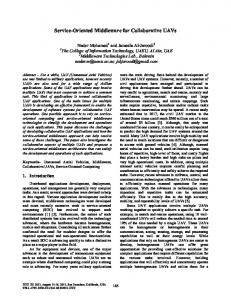
13.1. the
The hardware block diagram for the MUSIC Algorithm is shown in Figure As seen in this figure, the data collected from the sensors is utilized to form covariance
matrix.
The
eigendecomposition
is
performed
using
Householders transformation and QR method. The Eigenvalues are used to find
Sthe
number of sources and finally using the eigenvectors in Power method we find the angle of arrival. The Hardware block diagram for ESPRIT algorithm is
3
I
shown in Figure 3.2. It is similar to the MUSIC algorithm but instead of power method of MUSIC some more computations are performed to evaluate the angle of arrival in case of ESPRIT.
3.2 DATA COVARIANCE MATRIX FORMATION
3
Once the data has been collected by the sensors the data covariance matrix can be computed using
I
45
i1
Sensor
I I
M-1arianc Ho shod r Matrixtransformation
QR M ethod 1-0
I U Power Method
Direction of arrival
Angle of arr: al and number of sources
i
Figure 3.1: Hardware block diagram for MUSIC algorithm
4 I I I 3 I
i i I
I 46
i
I I I
ensor L
Covariance
i
Householders transformation
I I
O
,
Estimate the number of sources
Decompose
2
E = (e...ed
U
3
Householders transformation of o E
QR method for E
XY
Partition of matrix E into 4.4 Matrix
I I method
I
I j
Figure 3.2: Hardware block diagram of ESPRIT algorithm.
i
1
47
n Xx(p).x(p)* R XX =
n
Where
R × x(p)
n! Covariance of data matrix
=
Vector of data output from every sensor at pth sample
=
given by (x I, x 2. n
(3.1)
. . . .
.. x 8 )T
g
=Number of samples
The sampled data obtained from the sensors is used to obtain the data covariance matrix given by equation (3.1).
For instance, the element (ij) of Rxx
denoted by R ij is computed as:
n
n xi
n
(p) x1 (p) .
1
P=
Since the covariance matrix is Hermetian, the computation of lower triangular matrix of covariance matrix is sufficient to get complete information of the full matrix.
The parallel computation of the data covariance matrix is performed using systolic architecture.
As stated earlier the covariance matrix is Hermetian and
computation of lower triangular elements of the covariance matrix is sufficient to get the information for the entire matrix. Since there are 36 elements in the lower triangular
8 x 8 matrix, systolic architecture will have 36 processors.
Here a
triangular arrangement of the systolic array with global routing is considered as shown in Figure 3.3.
Each processor is numbered as Pmn where m is the row
number and n is the column number. The sampled data from the ith sensor is sent
48
3
IA/D
A/D
A/D
A/D
PEI IPE21
PE22
IPE31
PE32
IPE81
P3
4PE82d
PE874
I
do i=1,p As AS
I IFigure
Aend
S=S+A.B do
B 3.3: Architecture for Computation of Covariance Matrix
49
to the
ith
from the
row and the 3rd
ith
column simultaneously. For example the sampled data
sensor is sent to all the processors in the third row and the third
column. Each processor performs multiplication and addition of two sampled data in parallel in all the processors for every clock cycle . Since there are 36 processors, 36 multiplications and 36 additions are performed simultaneously. Each processor has a memory to store the product of multiplication which is added to the product obtained during the next data cycle. Once the operations of multiplication
and
! I 3 I
3 3
addition for all the sampled data in all the processors is performed, the stored data in each processor is then divided by the number of samples in all the processors in parallel. The resulting output are used to form the data covariance matrix R
3.4 HARDWARE FOR HOUSEHOLDER TRANSFORMATIONS
3
As shown in Chapter 2, the determination of all the d and the new elements of the
I
columns of the matrix can be computed in parallel. A modified architecture is proposed for the computation of the tridiagonal matrix. Thus this algorithm can be mapped on a hardware architecture with the number of processors equal to m+1, where m is the order of the matrix. Arrangement for 8 x 8 matrix is as shown in Figure 3.4. The columns of the matrix are sent to each processor in a pipelined fashion in reverse order such that the last element of each column becomes the first element. The Processor PEI is used to find the w and c required by other processors to find the d. Processors PE2, PE3... PE8 are used to find d using the value of w and c
3 3
3 5
found in the first processor. At the same time the first processor is used for the evaluation of 3. The first element of the first column and P are the output of the first iteration which are used as input for evaluation of eigenvalues using QR method. All the d , are evaluated in parallel and are sent to
50
3
I
Ii&r
PE CoI CoI I-i Io Ip IE Co o
P P
PEI
CoI
+
51
I I the processor PE9. The processor PE9 is exclusively used for the determination of v
£ 3
using d and w. The v are then routed back to all the processors. The processors PE2, PE3... PE8 use w, d and v to find the new values of the elements of the columns in parallel. The counter is used to set the number of iterations to
m-2.
For m-2
5
times, the intermediate results are used in feedback loop and the same set of processors are used repeatedly. The feedback loop has a FIFO memory to temporally
I
store all the elements of the column until operations on previous iteration are completed. For the first iteration, operations on 8 x 8 matrix are performed hence all the processors are utilized. For the second iteration, operation on 7 x 7 matrix are
3 3
performed. Now the first column of the matrix is already computed; therefore new elements of the second column from PE2 are fed back to PE. Thus for the second iteration, PE2 does not have any column to work on and is thus disabled. All other processors perform same operation as in the first iteration, but the elements of each
I
column are reduced by one element. Thus for every new iteration the columns and the elements of the columns keeps on reducing.
3
3.5 PARALLEL ALGORITHM FOR THE TRIDIAGONAL QR ALGORITHM
I
3
The given factorization, if applied to a full m x m data covariance matrix Rx will result in the operational cost of every factorization being 0 follows from the QR algorithm where by setting A1 = R,
(M 3 )
[421.
This
the first phase consists of
!
calculating an upper triangular matrix Rk and a unitary matrix Qk such that Ak = Qk Rk
and during the second phase, the product R k Q k is performed to obtain A
k+
I
k=l,..., n-I, where n denotes the number of iterations. For this reason, it is generally not feasible to carry out the QR transformations on R ,,, Instead, if R,,
is first
reduced to a tridiagonal matrix T using Householder's transformations, the subsequent transformations in chapter 2 will always give a tridiagonal matrix, and
52
i
5
3
I I thus, only (m-I) subdiagonal elements have to be eliminated to obtain the matrix Rk
i
during every factorization.
Thus, the cost of the eigendecomposition falls
substantially from O(m 3 ) to O(m) [42]. Furthermore,
Phillips and Roberston [15]
proposed a sequential algorithm for updating the entries of the tridiagonal matrix
i
without calculating, in the first step, the matrix
R
k
• Although this algorithm
reduces the processing time to some extent by avoiding the computation of R I
k
by
Q k at every iteration, and also the storage of the matrix Rk , but still every iteration in the algorithm requires
m steps. For n iterations, mxn
steps are required to
perform the eigendecomposition of the tridiagonal matrix. For the case of a matrix
I
of order 8 and for 11 iterations, various steps are shown in Figure 3.5, where (ij)
I
th
denotes the pairs of a(i,.) and b(i, .) at the j step.
At every step, one pair of a's and b's are computed. For example, in step 5 a(5,1) and b(5,1) are computed.
Every iteration
requires
eight steps . The last
elements shown in Figure 3.5 are a(8,11) and b(8,11), and they are computed after 88 computation steps.
I
In this section, an attempt is made to parallelize this sequential
algorithm to reduce the number of steps from mxn to 2(m+n)-10 steps.
A
parallel/pipelined algorithm has been developed and is described in terms of a simple program consisting of odd and even steps.
Iterms
During an odd step, the odd
(a(i,.), b(i,.)), i=1,3,...m-1, of the matrix T given by (2.22 ) are updated in parallel.
Likewise, during an even step, the even terms a(i,.), b(i,.), i=2,4...,m, are updated in a
I
similar fashion. A pseudocode of this algorithm is given in the following:
i I
Step
I
1 2
Computation performed sequentially (1,1) (2,1)
1
53
6 7
((41) (5,)1),1
9 10 11 12 13
(1,2) (2,2) (3,2) (4,2) (5,2)
11
(632))
16
(74),8,))
13
(1511))
82 83
(2,11) (3711)
84
(4,11))
85 86
(5,11) (6,11)
87
(7,11)
88
(8,11)3
Figure 3.5. Example of the sequential algorithm for updating the entries a's and b's of a tridiagonal matrixI (matrix order = 8,number of iteration =11)
x(1,i)=0;b(1,i)=0;a(O,i)=0; b(m+1,i)=0;c(0,i)=1;s(0,i)=0;1 c(m+l,i)=1; s(m+l,i)=0; n = number of iterations for k= 1,n+(m-2)/2
Odd Steps3 for j=1,m-1,2 i=k-(j+1)/2
Update the a's and b'sI if (i n-1) b(j,i+I )=b(j,n)
I
~~
)ajn
~
I~+L)=sjli *j,0+~-Ii.aji else
if ( x(j+1,i) else
Ir=sqrt(
=
0)
S,=
Ib(j+1,i) I
+x(j+1,i) 2
c(j,i)=x(j+1,i) / r
I
~
~~~~endifs(,)b+1i)/
w'=c(j,i) x(j+1,i)+s*(j,i) b(j+1,i)
I I
v=c(j-I,i) c(j,i) b*(j+I,i) + s*(j,i) a(j-s-,i) b(j,i+1)=s(j-1,i) w a(j,i+1)=c(j-1,i) c(j,i) w + s(j,i) v Computations of eigenvectors
I I
for 1=1,m u(j,l,i+1)=c(j,i)u(j,l,i).+S*(j,i) u(j+1,l,i) u(j+1,l,i+1) =-s(j,i) u(j,l,i)+c(j,i) u(j+1,l,i)
end for endif end for Even steps for j=2,m,2 i=k -j/2
I I'
Computation of the a's and b's if (in-1) b(j,i+1 )=b(j,n)
a(j,i+1 )=a(j,n)
1
55
if ( x(j+1,i)
=
0)
else 2
2
r=sqrt( i b(j+l,i) I +x(j+1,i))3 c(j,i)=x(j+l,i)/r
endifI w=c(j,i) x(j+1,i)+s*(j,i) b(j-,-,i) v=c(j-l,i) c(j,i) b*(j+1,i) + s*(j,i) a(j+1,i)3 b(j,i+1)=s(j-I,i) w a(j,i+l)=c(j-I,i) c(j,i) w + s(j,i) vp Computations of eingenvectors
for 1=1,m3 u(j+1,l,i+1) end for
=
-s(j,i) u(j,1,i)+c(j,i) u(j+1,l,i)
end if enfrend for
An example of this algorithm applied to a matrix of order 8, and for 11 iterations is
shown in Figure 3.6, where (i ,j) is defined earlier.g
56
5
I I 11
Step
2 3 4 5 6
Compuations performed in parallel (1,1) (2,1) (1,2)
(3,1)
(2,2) (1,3)
(4,1) (3,2)
(2,3)
7
(1,4)
8 9 10
(1,5)
(2,4)
(3,3) (3,4)
(2,5)
11 12
(1,6)
13
(1,7)
(3,5)
(1,8)
16 17
(1,9) (1,10)
21
(1,11)
22 23
(3,10)
(6,7)
24
(5,9)
(7,8)
(5,10)
(8,8) (7,9)
(6,10) (5,11)
(8,9) (7,10)
(6,11)
Ientries
(8,7)
(6,9)
(4,11)
25 26 27 28
(8,6) (7,7)
(6,8)
(4,10) (3,11)
(8,5) (7,6)
(5,8) (4,9)
(2,11)
(8,4)
(7,5) (6,6)
(4,8)
(2,10
(8,3)
(7,4)
(5,7)
(3,9)
(8,2)
(6,5)
(4,7)
(8,1)
(7,3)
(5,6)
(3,8)
(7,2)
(6,4)
(5,5)
(3,7)
(7,1)
(6,3)
(4,6)
(2,9)
19 20
(6,2)
(5,4)
(3,6) (2,8)
18
(5,3)
(4,5)
(2,7)
15
(4,3)
(6,1)
(5,2)
(4,4)
(2,6)
14
(5,1) (4,2)
(7,11)
(8,10) (8,11)
Figure 3.6. Example of the parallel/pipelined algorithm for updating the
a's and b's of a tridiagonal matrix (matrix order = 8,number of iteration = 11)
In the following, some of the computations performed by this parallel/pipelined algorithm are given below
IComputations
performed during stepl
Sx(2,0)=-s(5,7).b*(1,O)+c(OO).a(1,O)
I
57
if ( x(2,O)
=
0)3
C(1,0)=1
eles(1,0)=0 r=sqrt( I Ib(2,0) 1I2 +x(2,0) c(1,0)=x(2,O)/r edfs(1,0)=b(2,0)/r w=c(1 ,0).x(2,0)+s*(1,0) b(2,00) v=c(0,O) .c(1,0) b*(2,0) + s*(1,0) a(2,O)
b(1,1)=s(O,O) .w1 a(1,1)=c(O,O) c(1,0) w + s(1,0) v Computations performed during step 2 x(3,0)=-s(1 ,0).b*(2,O)+c(1 ,0).a(2,O)3 if ( x(3,0) = 0) c(2,0)=1 else
s20=
r=sqrt( I Ib(3,0) 1 1 +x(3,O) 2) c(2,0)=x(3,O)/r
edfs(2,0)=b(3,0)/ r3 w=c(2,0) x(3,0)+s*(2,0) b(3,0) v=c(1,0),c(2,0) b*(3,0) + s*(2,0) a(3,0) b(2,1)=s(1,0) w a(2,1)=c(1,0) c(2,0) w + s(2,0) v Computations performed during step 3 x(4,0)=-s(2,0).b*(3,0)+c(2,0). a(3,0)I If( x(4, 0) = 0) c(3,0)=l s(3,0)=0 else r=sqrt( Ib(4,0) I +x(4,O)) c(3,0)=x(4,0)/ r s(3,0)=b(4,0)/ r
endif w=c(3,0) x(4,0)+s*(3,O) b(4,) v=c(2,0) c(3,0) b*(4,0) + s*(3,0) a(4,0)
58
5
I b(3,1)=s(2,0). Ix(2,1
a(3,1)=c(2,0) c(3,0) w + s(3,O) v
)=-s(O,1).b*(1,1 )+c(0,1.al)
if ( x(2,) =O0) c(1,1)=1 s(1,1)=O else r=sqrt( Ib(3,0) I +x(3,0)
I
c(1,1)=x(2,1L)/r
s(1,1 )=b(2,1)/r endif w=c(1,1).x(2,1)+s*(1,1) b(2,1) v=c(O,1) c(1,1 b*(2,1) + s*(1,1) a(2,1) b(1,2)=s(O,1) -w aQ1,2)=c(O,1) c(1,1) w + s(1,1) v Computations performed during step 4
I(,)-(,)b(40+(,)a4O I c(4,0)=1 I2 2 I if ( x(4, 0)
=
0)
ele s(4,0)=0
r=sqrt( Ib(5,0) I +x(5,0) c(4,O)=x(5,) / r
s(4,0)=b(5, 0)/r
endif w=c(4,0).x(5,0)+s*(4,0).b(5,0) v=c(3,0).c(4,0) b*(5,0) + s*(4,0) a(5,0) b(4,1)=s(3,0) w a(4,1)=c(3,0) c(4,0) w + s(4,0) v
I I
x(3,1)=-s(1,I ).b*(2,1 )+c(1,1).a(2,I)
if( x(3,1) = 0) c(2,1 )=1 s(2,1 )=0
else r=sqrt( Ib(3,1)1I +x(3,1))
I
c(2,1)=x(3,1)/r s(2,1)=b(3,1)/r
endif
I
59
I w=c(2,1) x(3,1)+s*(2,1) b(3,1) v=c(1,1) .c(2,1) b*(3,1) + s*(2,1) a(3,1) b(2,2)=s(1,1) w a(2,2)=c(l,l) c(2,1) w + s(2,l) v
I
The algorithm updates the pairs of a's and b's in the following manner Step I and 2
one pair
Step 3 and 4
two pairs
Step 5 and 6
three pairs
Step 7 to step 22
four pairs
Step 23 and 24
Three pairs
Step 25 and 26
two pairs
Step 27 and 28
one pair
3 3
I
This algorithm is also suitable for VLSI implementation, using an array of m/2 processors Prj, Pr 2 ,,..., Pr
and (m+2 ) cells clo, cl,..., cm+l constituting a
m/2
local memory, as shown in Figure 3.7. Each processor in the array performs certain computations such as floating point operations and square roots.
3 3
If the pairs ( a(i,.), b(i,.)), ( c(i,.), s(i,.)), i=0,2,...,m+l , are stored respectively in cl0 c11,..., clml, then during an odd step , each processor Pri, respectively 1) accepts a) c(2i-2, k ), s(2i-2, k ) from cell cl
3
2i-2
b) a(2i-1,k), b(2i-l,k) from cell cl 2i-1
3
c) a(2i,k), b(2i,k) from cell cl 2i 2) computes x(2i,k), c(2i-1,k), and s(2i-1,k) 3) updates a(2i-1,k) and b(2i-l,k) to become a(2i-1, k+1) and b(2i-1, k+1) respectively 4) stores c(2i-l,k), s(2i-1,k), a(2i-l,k+l), and b(2i-1, k+1) in cell cl
2i-1
and during an even step, each processor Pr i, respectively
I 60
3
U U 1) accepts a) c(2i-1, k ), s(2i-1, k ) from cell
Sc) 3-
C12i-1i
b) a(2i,k), b(2i,k) from cell Cl2i a(2i+l,k), b(2i+l,k) from ceil cl2i
1
2) computes x(2i+l,k), c(2i,k), and s(2i,k) 3) updates a(2i,k) and b(2i,k) to become a(2i, k+1) and b(2i, k+1) respectively 4) stores c(2i,k), s(i,k), a(2i,k+l), and b(2i, k+l) in cell cl 2i
In the first step of the algorithm, the pairs (c(0,0)=1, s(0,0)=0), (a(1,0), b (1,0)), and (a(2,0) , b(2,0)) stored in clo, cl and c12 respectively, are entered in the first
3 3
processor Prj. These values are used to form x(2,0), and to compute c(1,0) and s(1,0)
3b(
c(0,0), s(0,0), x(2,0), a(2,0) and b(2,O) 1,1)
I
according to the algorithm. These two values (c(1,0),s(1,0)) are stored in clto be used during the next step. The computed values of c(1,0) and s(1,0) are used along with
3and 3 I 3 5
to update a(1,0) and b(1,0) to become a(1,1) and
At the second step, the first processor accepts c(1,0), s(1,O), a(2,0) , b(2, 0), a(3,O) b(3, 0) to update in a similar fashion a(2,0), and b(2,0) to a(2,1), and b(2,1).
At the third step, while the second processor is updating a(3,0) and b(3,0) to become a(3,1) and b(3,1) respectively, the first processor is used to update a(1,1) and b(1,1) to
become a(1,2) and b(1,2) respectively.
At the fourth step, the second and first processors update in parallel the two
pairs (a(4,0), b(4,0)) and (a(2,1), b(2,1)) to (a(4,1), b(4,1)) and (a(2,2), b(2,2)) respectively.
The algorithm proceeds in this fashion so that the array is updating the entries of
I1
361
1 I the tridiagonal matrix in a pipeline fashion in the iteration as shown in Figure 3.8 for m=8 and for 11 iterations.
It can be noticed that after 28 steps, the updated entries of the matrix T are obtained. This result can be generalized to any matrix of order m, and for any
3
number of iterations n, where it is not difficult to show that 2(n+m)-10 steps are needed to achieve the desired result. Although, the preceding method would serve to correctly obtain the updated entries after a fixed number of iterations, it can be extended to accomplish
the same task for an unlimited number of iterations, until
i
3
the convergence is satisfied.
The previous array , shown in Figure 3.9, can be extended to include another m/2 processors P1 ,P 2 -...,Pm/2 , as shown in Figure 3.9, to update the matrix of the eigenvectors.
Given
the matrix
U= N H ,
transformations, and the matrix Q = Q, Q2
...
obtained
from
Householder's
Qn, where n is the number of iterations.
I
3
The product of Q H by U, to obtain the matrix of eigenvectors of the original problem, may be computed also in 2n+m-2 steps. If each column of the matrix U = N H is stored in an array of m elements consisting of a FIFO as depicted in Figure 3.8
I
, then during an odd step, the values stored at the top of the independent pairs of
I
arrays (1,2), (3,4),..., (m-,
I
m) are transfered in parallel to the processors
P1 ,P 2 ,
..,Pm/2 respectively. The rotation parameters generated during this particular step are also
sent
to the corresponding
processors. That is, the rotation parameters
3
generated by Pr1 are sent to P1 , and the rotation parameters generated by Pr 2 are sent to P 2, and so on. Once the top elements are updated, they are transferred to the bottom of the corresponding arrays The procedure continues until all the elements stored in the array are updated This is depicted in Figure 3.6(a).
I
3
Similarly, during
I 62
3
I I an even, updating the entries of the independent column pairs (2,3), (4,5),..., (m-2,
I
m-i) is shown in Figure 3.6 (b)
1
3.6 HARDWARE IMPLEMENTATION OF THE POWER METHOD Once the eigenvectors have been computed, the values of the eigenvectors are utilized to calculate the power
PM (0) = a*(O) E hE* n a(0)
(3.2)
As seen from this equation the evaluation of a*(0) E nE*n a(0) requires squaring of the product of rowvector of a(0) and the eigenvector matrix E n . Hence the product of a(O) and E , is evaluated and then the product obtained is squared and accumulated for all the values in the array manifold.
The hardware design is
shown in Figure 3.10. It consists of a set of 8 processors. Each processor finds the product of a(0) and columns E n in parallel. The product obtained is then summed using adders. The evaluation E* n a(0) is similar to the evaluation of a"(O) E n and hence the product of a*(0) E n is squared and added. The angle of arrival is thus calculated for different values of the array manifold. This computed value Q m (0) is inverse of P m (0) is different for different angle.
The angle for which Q m (0) is
minimum is the angle of arrival.
3.7 CONCLUSIONS Flow diagram for the entire MUSIC algorithm is shown in Figure 3.11.
Different
stages in the MUSIC can be substituted by different hardware architecture as
Iexplained
I
above. Hence the entire pipelined stage of MUSIC algorithm consist of
63
U 1) Data covariance matrix stage
5
2) Householders stage 3) QR stage 4) Power method stage
3 I
Various stages along with buffers ate explained in next chapter.
I I i I I i i I U i 64
i
Ecl 1 111 C
c13
c14
c17
c15
c18
(a)
(b)
I I
~
c (i,k) a(i,k) b(i,k)
s(i,k)
-~)A
s(i-l,k)
a(i,k+ 1) b(i,k+1)
)xilk=s~-~)b(~)cilkaik
a(i+lI,k)
~ ~~
if (x(i+1,k) = 0) c(i,k)=1. ess(i,k)=O.
r = sqrt(I b(i+1,k)I1.I1b(i+1,k) I + x(i+1,k). x(i+1,k)) c(i,k)= x(i+1,k) /r s(i,k)= b(i+1,k)/r end if w= c(i,k) x( i+1,k) +s*(i,k)b(i+1,k)
I
v= c(i-l,k)c(i,k)b*(i+1,k) + s(i,k)a(i+l,k) b(i,k+1)=s(i-l,k) w Figure. 3 . Updating the eigenvalues, (a) odd steps, (b) even stepsa(i,k+lI)=c(i-1,k)c(i,k)w+s(i,k)v
Figure. 3.6. Updating the eigenvalues, (a) odd steps, (b) even steps
*
65
prl r2 p3 Pi P2P3
IFI pI P
Figure.3.6 (a) Updating the eigenvectors during an odd stepI
c~i~kI s(i,k)
u(i,jk+1 )= c(i,k) u(i,j,k)+s*(i,k) u(i+1,j,k)
p Iu(i+l,j,k+l)=
u(i,j,k)
-s(i,k) u(i,j,k)+c(i,k) u(i+l ,j,k)3
u(i+l1,j,k)3
u(i,j,k+I) JFu(i+l,j,k-.-)
66
3
I
~
~I
C11
c12
Ir P
c13
c14
r 2P
c15
C16
c17c1
r
Iiue36() paigteegevcosdrn nee tp
I6
r
9
a(e)
PE I Col PEI2 Col 3 PE 3 Col 4 PE 4 ] 1 5 EI Col
Col
PE8Pm
(8)
Figure 3.7: Hardware For Power Method
68
Chapter 4 DEVELOPMENT OF ARCHITECTURE FOR MUSIC ALGORITHM AND GENERALIZED PROCESSING ELEMENT
4.1 PIPELINED STAGES AND BUFFERS IN MUSIC ALGORITHM
The MUSIC algorithm is executed using four pipelined stages namely the covariance matrix formation, Householder method, QR method and the power method as stated previously. shown in Figure 4.1.
These pipelined stages along with buffers are
The covariance matrix stage which is the first stage collects
the sampled data from 8 different sensors and computes 8x8 covariance matrix. The covariance matrix has 36 processors, all of them perform the same operation in parallel. The Householder method which reduces the covariance matrix to a
I
tridiagonal matrix forms the second stage. The data generated in first stage is pipelined to the second stage through eight FIFO buffers. These FIFO buffers store data for transfer to the Householder stage. Householder method has 9 processors.
The hardware for the
PEI to PE8 perform computations on
each column of the covariance matrix and PE9 is used to compute data required by other processors. The tridiagonal matrix is reduced to a diagonal one by QR
I
method which forms the third stage. Data generated by PE1 of second stage is pipelined to PEI of third stage through a two word deep FIFO. The third stage
I
has 2 kinds of processors, PEl which computes eigenvalues and PE11 to PE18, which compute eigenvectors. Each processing element PE11 to PE18 generates
I I
eight eigenvectors which form the rows of the 8x8 eigenvector matrix. Eigenvectors computed by the third stage are pipelined power method which forms the fourth stage.
It has eight processors PEI to PE8 and each processor
works on the array manifold and the column of the
1
69
Sensors ~I
DD-DD D MD-DE DDDDD7
Covariance Matrix Stage3
I I
'I FIFO Buffers
Householderstage
8
4
7: " 6
I
3-2-
I
I
I
1I/(O)
Figure 4.1 Various Stages and Buffers in MUSIC AlgorithmI
I
I I Ieigenvector matrix.
Since QR method produces rows of the eigenvector an
hardware switching method is used to convert rows to column before passing on to power method stage.
Power method has 8 processorsthe eigenvector matrix
needs to be output of PE8 gives the inverse of the power. output for different angle of the array manifold.
Igeneralized PE architecture is described. I4.2 THE GENERALIZED PROCESSOR
I 1processing
This PE8 produces
In the following section, a
As seen above there are four pipelined stages with eight different kinds of elements. All these processors perform similar arithmetic functions.
Thus, various functions performed by different processors can be grouped
Itogether and performed by one generalized processor. Therefore instead of using Ieight different processors, a single generalized processor can be used.
IThe generalized processor named GP, has an architecture which is designed to maximize the throughput for different PEs required in the MUSIC Ialgorithm. The internal architecture of GP has the capability to execute various Ioperations in the MUSIC algorithm. After studying the capabilities required for the different PEs, a list of the following six arithmetic functions is compiled.
I1)
Addition 2) Subtraction 3) Multiplication
14)
Division 5) Multiplication, Addition and Accumulation
I6)
I
Square rooting
71
I I Hence instead of using a generalized Arithmetic Logic Unit (ALU) as used in commercially available microprocessors, a block of three specified arithmetic
I
functional units are utilized. These functional units are:
g
1) Addition/Subtraction Unit
3
2) Multiplication/Division Unit
3
3) Square Root Unit. Computed data can be stored temporarily in embedde. (RAM) or sent to the output port.
"andom Access Memory
The operation of data storing and I/O is
3
performed using data bus.
The processor has eight, 16 bit general purpose registers. These registers
I
are named as A, B, C, D, E and F. Each 16 bit register can also be used as two 8 bit registers in concatenation. It also has two index registers X and Y.
Each index
register is 8 bits wide. GP also has a 8 bit program counter (PC) and program status word register (PSW).
3
U
Thus the major components of the generalized processor GP are as follows: 1) Address bus
I
2) Data bus 3) Floating point adder/ subtracter.
I
4) Floating point multiplier/divider. 5) Square rooter. 6) Embedded data memory.
3
7) Two Input ports. 8) Two Output ports.
I
9) Control unit
72
3
I I The above mentioned components along with the arrangement of the registers is
Ishown in Figure 4.2 and each of them are explained as follows:
I I
-A
I N
I JII 112
3
sensors' output while the second level of DPRs will be in read mode where previously stored information is now being used to compute one vector product X(nTdL) with its conjugate transpose. Addresses needed by the DPRs are provided by counter I, counter J and a 3-bit counter which is controlled by a 9-bit counter. Two multiplexors, controlled by S (or S), direct the needed address to the DPRs. If the DPRs are in write mode, the 3-bit address is selected, otherwise, address I and address J are selected. In read mode, the data addressed by counter I is supplied from each DPR to the respective register, while simultaneously the data addressed by counter J is supplied from each of the same DPRs to the respective processing element. Counter K is initialized to the value of zero and then is used to broadcast the output of one of the registers, one at a time, to all of the eight processing elements. Each PE then multiplies that register output data with the value already stored in its internal register (an element of vector J). The multiplication result is added to previously computed values that are stored in memory at an address pointed to by counters I, J and K. Counter K loops through its range (0-M7) to construct an 8x8 sub matrix. Counters I and J loop through their range (7--+0) to compute the 36 sub matrices. At the end of three loops (I, J, K), the assignment of the two levels of DPRs are switched and the operations performed by the PEs are repeated for the newly available data. The process is repeated 600 times to build the required matrix. The covariance matrix is formed by collecting the matrix and dividing its elements by 600. Figure 5.11 shows the control lines for each Dual Port RAM (DPR). Since the architecture is designed to perform one sub matrix at a time, it is possible to detect when the PEs finish the computations of that sub matrix. At that time counter K reaches its highest state (K= 7 10=lllb) . If at that time counter J is indexing the last column (J=000b), the computation of the lower triangular matrix is complete. This logical function is implemented using two AND gates and one NAND gate. The output of the AND gate is used as a clock input to the D flip-flop. The value stored in the flip-flop is 113
Counter
~To set #2 of DPRs reea/wwrieeconttool ANDW
AdrsBDRAddress
Enable/DisableOR
fo -- -- -
o.If Data B
Figure 5.11
Data A
-- 9-bitcownter
S = I = read mode then enable else if A5A8 then enable else disable
Dual Port RAM control block.I
114
I I used to select one level of the DPRs; either the top level or the bottom level, while the
I
inverted output S of the flip-flop is used to select the second level of the DPRs. The selection is meant to be used as a read/write control. Notice also, that there is an
Ienable/disable
control on a DPR. The only time that the chip should be enabled is when
it is time to read information for processing (S=I), or when it is time to write the newly read sensor output data (S=0 write mode). An OR gate is used to enable the DPRs.
I
When a DPR is in read mode, it receives address I and address J. On the other hand, when the DPR is in write mode, it receives its only address from a 3-bit counter
Icontrolled by the 9-bit counter (see Figure 5.10).
The internal structure of each processing element is shown in Figure 5.12. As illustrated, the following hardware elements are needed:
I
Four Multipliers Four Adders
IThree Registers One of the values stored in the external registers is broadcasted to all the PEs. Complex multiplication of the value with the data stored in the internal register is performed.
IFour
multipliers are needed due to the complex nature of the data. It is also desirable to
use as many multipliers to generate parallelism to enhance speed of the system. Two adders are used to add the results of the complex multiplication; one adder for the real part and another for the imaginary part. Previously calculated data that has been stored in memory, is retrieved and fed through two sets of registers before it is added to the newly computed complex data. It is possible to eliminate the latter two registers to
I
I115
I
minimize the number of hardware needed in each PE provided that all the propagation delays have been accounted for in the multiplier then the adder stages.
i
I CONCLUSION
I
In this chapter BASS-ALE algorithm has been simplified and converted into parallel/pipelined algorithm. First part of this algorithm requires computation of covariance matrix. Three architectures are proposed and an architecture with 8 PEs has
3
been selected for detailed design. Design for the next module is in progress and other parts are being designed separately.
i I i I I i
I i I ! I i 116
3
Real 1 Imag 1
"from memory" Real3 Imag3
'firom broadcast" Rea12 Imag2
"from DPR' Real 1 Imag 1
Real 1
Rea12
x
Figure 5.12
Imag 1lImag2
x
Reall1
mag2
x
Rea12 Imag I
Real3 Imag3
x
Detailed internal structure of a Processing Element.
117
! I Chapter 6
I
DOA ESTIMATION FOR BROADBAND SOURCES USING A BILINEAR TRANSFORMATION MATRIX APPROACH
3
6.1 INTRODUCTION The estimation of angle of arrivals of multiple broadband sources has been carried out in a variety of ways over the past few years. The conventional
3
approach is to form a generalized correlator [311 to estimate the Time Difference Of Arrival (TDOA) of the signal at the sensors. The so called maximum likelihood based methods [32-34] require knowledge of the source and noiseI spectra and are computationally expensive. The parameter estimation based methods [35-371 assume Auto-Regressive Moving Average (ARMA) models for
I
the received signals and the estimated ARMA parameters are utilized for the TDOA calculations. Such model based methods have computational complexity and their effectiveness depends upon the approppriateness of the model chosen
n
to represent the unknown broadband signals. Another way is to extend the ideas from the narrowband case [381 and use a eigendecomposition approach for the
3
estimation. This approach involves the incoherent combination of the eigenvectors of the estimated spectral density matrices at each frequency bin to
a
calculate the TDOAs. One other way [39,40] is to use the initial estimates of the
3
angles oi arrival to transform the eigenspaces at different frequency bins and generate a single coherent subspace which is eigendecomposed to give more
I
accurate estimates. Well separated angles can be estimated by focusing at different angles at each time and iterating to obtain the accurate results. Shaw and Kumaresan [261, proposed an algorithm for broadband DOA
3
estimation using a simple bilinear transformation matrix. An approximation
8
3
resulting from a dense and equally spaced array structure is used to combine the individual narrowband frequency matrices for coherent processing. When compared to other coherent approaches, this algorithm has the advantages of being non-iterative and does not require any initial estimates of the angles of arrival and all angles are computed from a single step of coherent subspace calculations. Hence it was found to be a suitable algorithm for computation of DOA using dedicated hardware. The algorithm has been described in the following section. 6.1.1 Problem Formulation Consider a linear array with 8 sensors which are spacedat equal distances. The incoming signal is assumed to be composed of d plane waves emitted from d sources (d < 8), with an overlapping bandwidth of B Hz. The signal from the kth sensor is expressed as d
si(t - (k -1) - sinOi) +
rk (t) -
Ilk
(t)
(6.1)
i= I
T
T
2
2
~
where si(.) is the signal radiated by the ith source, A is the separation between the sensors, c is the propagation velocity of the signal wavefront, O1 is the angle that the ith wavefront makes with the line of array and nlk is the additive noise at the ith sensor. Performing the FFT and representing the two sides by their Fourier coeffficents
119
d
e-jit
Rk (W!)
(k-1)'A sinO, Si (w, ) + Nk
(W1 )
(6.2)
i=1
with wV =
,lI+tf, where wzVand w,.. are the frequencies which span
2n
the bandwidth B.
3
Writing in the matrix notation
I 3
R(wI) = A(wt ) S(zol ) + N(w)
(6.3)
where these matrices are composed of the column vectors
I
R(wt ) = [r1 (wt ) ...r8(wt )IT
(6.4a)
N(O ) = [nj(wt ) ... n8(wt )]T
(6.4b)
) = [si(w ) ... s,(Zt' )IT
(6.4c)
S(w7
I
and the matrix A(zv ) is a 8 x d direction finding matrix
Fe A(zvl )
1
...
=
e-17zvt r,
T,
=csin 0,
... '
jw
I
1
...
(6.4d)
e'j~Zwdrt-]
I
(6.4e)
tj being the TDOA of the ith source. Assuming that the observation time is large
i
enough when compared to the correlation time of the processes, the covariance
I 5
matrix of the Fourier coefficient vector r(wi ) will approach the spectral density matrix
12103
K(wj ) = A(w, )P,(w1 )A"(w,) + (Y,,
Po(wI )
(6.5)
where K(wj), P,(wt ) and P(wl ) are the spectral density matrices of the processes r, ()Sk(.), ni (-)respectively. The noise process is assumed to be independent of the
sources and the noise spectral density matrix except for a multiplicative constant UPI The problem now reduces to the estimation of the
t1 '
s from the
covariance matrices K(u'1 ) and the noise representations. Then the angles of arrival can be computed from the Equation (6.4e). 6.1.2 Problem Solution This particular approach utilizes a bilinear transformation and dense array approximation to form the transformation
matrices.
The bilinear
transformation matrix that is used can be synthesised from the coefficients of the polynomials pk(z) = (l+z)M-k (l-z)k-1, where k =1, 2, ... M-1. M here indicates the number of sensors that the system is using, which in this case is equal to 8. Hence the transformation matrix in this case is an 8x8 matrix, the synthesis of which is shown in the next section. E(w, ) denotes a diagonal matrix given by
E(wi
=
[
...
L
(6.6)
(1+e-,7v ir,,)7
Premultiplying A(wi ) by the transformation matrix B and simplifying the product gives
1 I -
1..
1
-
BA(w )2
j
2
(j tan--..-)
E(w)
(6.7)
itan--T-2
I
Assuming that the sensor to sensor separation A is small when compared to the wavelengths of the incoming signals, tan- - can be approximated by 2
7VI
Now consider an 8x8 diagonal matrix D( IL) whose (kk) th term is given by dk, =( L7 L;)k-1
1 3
(6.8)
where Wc =2 7Efc and fc is the midband frequency of the signals.
3
It can be approximated as D(
WI
)BA(wi ) =
... (wvcr, )7
.
...
c ...
1cI
E(w,)
(6.9)
i
(zvcrd )7_
There is a new matrix A(wc ), whose columns are the transformed direction
3
frequency vectors which are dependant upon Wc rather than w, . The columns of the matrix are linearly independant as long as r i *rk for i *k. A new transformation matrix is defined as T(-
)=D(-
)B
I
(6.10)
This does not depend upon the arrival angles and can hence be computed
I
independently of the angles. Using these transformation matrices for each
I 1..2.3
individual narrowband frequency, all the spectral estimates can now be combined at the midband frequency in the following manner; 11 +nf
T (w ) K(w ) TH(w, )
G=
(6.11)
I=Ii
11 +ni
and
Gn= Y T (w) Pn (wt) TH(zv)
(6.12)
1=11
Then the coherent signal subspace theorem for the matrix pencil (G,G,,) is used to estimate all the angles of arrivals by computing the maximas of the measure given by J(O)
=
1
8
1
I ae(wc)ek(wc)
(6.13)
12
k=d + I
where ek(V, ) denotes the generalized eigenvectors of the matrix pencil (G,G,, ), which correspond to the 8 - d eigenvalues, and a0 (w, ) represents the new direction frequency matrix.
123
I 3 I
6.2 PARALLELIZATION AND MODIFICATION The first objective in the implementation of such signal processing algorithms is to modify them in such a way so that the maximum possible parallelism and pipelining can be achieved which would enable the real time
3
implementation of the algorithm. The modification of the algorithm outlined in the previous section takes into consideration the various tradeoffs involved in the ultimate realization of the hardware like the timing and cost considerations
3
which would make the project viable. A flow chart of the modified algorithm is shown in Figure 6.1(a). Figure 6.1(b)
I 3
shows the mathematical transformations that the algorithm involves.
There is a linear array of 8 sensors which are sampled at a rate of 80 samples per sec. A segment of 64 samples is considered which form the single step input to the next stage of the FFT processors. As shown in Figure 6.1(a) a single
I
estimation of the angles of arrival involves the processing of 64 such segments of
I
64 samples each.
After 64 samples are collected, the next step involves the
3
transformation of these signals from the time domain to the frequency domain by performing a 64 point FFT. The output is a 33 element vector in the frequency
3 3
domain which is representative of the input signal at that sensor. The next block is the calculation of the covariance matrix at each frequency bin. Essentially the covariance matrix consists of the product of the frequency vector and its Hermetian which is obtained from the corresponding elements in the FFT output vectors. Hence for the 33 different narrowband frequencies there are 33 different covariance matrices independant of each other. These matrices
3
are averaged over the 64 segments before being passed on to the next step in the
12d4
PRECOMPUTATION Estimation of noise spectralFT density matrices
S
* *
64 Loops Formation ofFomtnad Transformation
Fomto
matri~es
T
and
averaging of coariance matrices ........
(w,
CompuaA
o
Compta~i.~ o
Comutaton
o
Coputaion
f
GG
Cholesky
L andFowr
decomposition L
TSubstitution JI
Householders
Power method Estimation of angles of arrival)
Figure 6.1: Flowchart of Wideband algorithm
:33 Loops
I
_
_
__I_
__I
_I_
I
Collect X'U.(t) i=l .. 8; n= .. N Compute FFT for every Xni(t) X.((sL) L=L ... L ni
OL) Compute X *( j=I..m
I
l+nf
1
Xn (wuL)
k=j,..m
I
L=L ... L
Compute Average for
N3 1 x nl.((oL)X rk(L)
I
Y
N
n=1
Form H
N
A
K(wI)= 1 XX n O
X n (oL)
I
N n=l
... L
I=L,L+ 1
I
+nf
Compute L +nf
A
H
I
G = , T(o)L) K(wL) T(oL) L=L I
I
and H
Ll+nf
G=
X L=L
T(wL) Pn (wL) T(wL) 1
(Perform Cholesky Decomposition)
1
GX = A.G X Convert to the standard eigenvalue HY =XY
____________I
Perform eigendecomposition - position of (G, I) Continued...
1 126
Continued... Obtain m
I
estimated number of sources
estimate angle of arrival P(8) k~d+1
aD~ e(o)
~kc
V
where (0C
12
I I algorithm which is the projection of the covariance
3
matrices K(wi ) onto the
single midband frequency in the spectrum to compute the G matrix. The computation of the G matrix requires the transformation matrices T(w1 ) which are precomputed
as shown in the diagram.
I
3
As seen from
Equation(6.8) in the previous section the computation of the matrix involves the
3
knowledge of the narrowband frequencies in the bandwidth. Given a specific problem such an estimation of the frequency bins is made by splitting the bandwidth into 32 equal parts and taking the frequencies at the boundary. With
3
this initial assumption of the narrowband frequencies in the spectrum of the incoming signals the transformation matrices can be computed offline. This is
3
possible because the matrices are unique for a set of frequencies and are independant of the angles of arrival of the incoming signal.
Hence these
invariant matrices can be stored in a ROM for a dedicated architecture and can
3
be called up whenever they are required during the processing. However an architectural model has been developed to compute the transformation matrices on line which would enable the system to be more general purpose and allow it to run scans over different frequency ranges without the initial knowledge of their frequency components. The computation of the actual
I 3
transformation
matrices is outlined below following the principles explained in the previous chapter. 6.2.1 Computation of the Transformation matrices
pk(z)
The transformation matrix is derived as follows:
U
Let B be a matrix constructed from the coefficients of the polynomial
I
(I+Z)k (I -Z)8-k,
where k =1, 2, ... 7. K denotes the number of the row of the 128
8 x 8 matrix which is formed. In this case the nonsingular matrix has been computed and is shown below 1 721 35 1 5 9 5 1 3 1 -5 1 1 -3 -3 B=1 -1 -33
35 21 -5 -9 -5 1 3 3 3 -3
7 1 -5 -1 3 1 -1 -1 -1 1
.4
1 -3 1 5 -5-1 3-1 1 -59 -5 -5 9 -5 1 -1-721 -35 35 -21 7 -Li From this B matrix the transformation matrix can be computed according to Equation (6.10). For the matrix D( w2
,
the (kk) th term is given by
2u )k-1
Let p denote the constant term such that
I
P-
2Wc w
The transformation matrix can now be written as shown in Equation (6.15) The matrix T can thus be computed and is stored in a ROM and is
Iretrieved I
by each processor. The next precomputation block is the calculation of
the G,, matrix which is the estimate of the noise spectral density that is expected to be present in the signal. The algorithm requires a previous knowledge of the
I
noise in the system
which is expressed in terms of the P,, matrices at each
frequency bin. The procedure for calculating involves two matrix multiplications
I
aj d is similar to the computation of the G matrix from the covariance matrices. The calculations are performed 33 times, once for each frequency component and
I
are then averaged at the midband frequency.
I
I 29
I 7p2 21p3 35p4 35p 5 21p p
p
5p 2 9p 3 5p 3p 2 _.p 3 _p
-5p
-5p5 _9p 5
7p 7
p
6
_5p7
.p8
_p6
p-3p _3 p 3p 3p 6 5 p-' -3p 3p 4 -3p =-_p2 p( p -p2-3p p 3-5p -p 6 p ~ .3 p 3 4 5 .32 p 2
1
6
3p 7
-p
7
3-pp77
p8
-p -p8
.7 3p 7
8
5 p4
.5p 5
-p 6
9p 3 .5p 4
.5p 5
9p 6 .5p 7
p8
7p 7
_p8
p3
P
.5p
p
6 -7p 2 21p 3 -35p 4 35p 5 -21p
(615
-p
1
3
The equation governing this transformation is shown below. 11+nf
Gn= J1T (w, ) Pn,,(W) T"(wi)
(6.16)
1=11
The matrix G,, is then stored in the ROM and accessed at the time of the
I I
Cholesky decomposition.
3
6.2.2 Computation of G
!
The G matrix which is the combination at the midband frequency of all the individual covariance matrices of different narrowband components requires the projection of these matrices by the transformation matrices and involves two
I
3
matrix multiplications as shown in the equation below. 11i+nfI
G=
T (we) K(w ) T"(w)
I=11
(6.17)
I
The process goes through 33 iterations as shown in the flowchart. Each loop involves two matrix multiplications which are done sequentially, because the input to the second operation is the output from the first. However parallelism has been achieved inside each operation as it is performed in one cycle. The computation of the G matrix gives the matrix pencil (G, G,, ) of which G,, has been precomputed. 6. 2.3 Cholesky decomposition The further processing of the signal requires that it be organised into a standard form so that certain standard operations of matrix algebra like the eigendecomposition can be performed. The algebraic manipulations which are performed to achieve the objective are described below. G,, and G are two matrices which need to be put in the standard form such that GX = XG,,X
(6.18)
where X = the eigenvalues of G X = the eigenvector matrix of G,, and G Decomposing G,, into G, = L LT
(6.19)
and substituting G,, in the equation and multiplying both sides by L- 1 gives L-1G L-T. LTX = X L- L LTX Defining
L-1 G LT = H and LT X = Y
(6.20) 131
I 3
The standard form required for eigendecomposition can be written as (6.21)
HY= XY
The decomposition G,, = L LT is obtained by doing the Cholesky decomposition
3 3 3
which is the next step in the algorithm as shown in the flowchart. The flowchart of the Cholesky decomposition is shown in Figure 6.2. The objective of reducing to a lower triangular matrix is achieved by computing the elements below the diagonal according to the equation i-i
aki-
aijaki (6.22)
aka
The diagonal elements are however computed by the form'ila k-I
akk=
-
akj
(6.23)
3
Once the lower triangular matrix L has been computed the transpose LT can be obtained.. The next step is to obtain the two matrices H and Y. This part
I
needs the calculation of the inverse of the lower triangular matrix L as is seen from Equation(6.20). This computation is both time consuming and complex
3 3
especially for real time applications. The ultimate objective is not to calculate the inverse and to circumvent this requirement, a simple algebraic manipulation is described below: Assuming a matrix W such that LW=G
1
(6.24)
3
we have
132
START
Ii
j=I
I i=i+1
GS
No
Figurea6.2 flwcar fo
hoek
eopsto J133
I W =L-IG Taking the transpose and premultiplying both sides of Equation (6.24) by L-1 gives L-1W =L-1 (L-1G)T
3 3
= L-1 GT ( L. )T
= L-1 G ( L-1 )T
(as G is Hermitian)
=HH
3
Hence LH = WT
(6.25)
Considering the two Equations (6.24) and (6.25) it can be seen that the
U 3
problem of computing the inverse is now reduced to the computation of the H matrix by two forward substitution operations. First the matrix W is computed from the Equation (6.24) as the other two matrices are known. Then it is transposed, which is a simple routing exercise in the architecture and use the result in Equation (6.25) to compute the H matrix.The computation of Y also
I
follows the same procedure. The resultant matrices can now be treated in the same manner as the narrowband case to compute the angles of arrival. First the Householders and QR transformations are performed to reduce the dense matrix
3
into a diagonal one and then the power method is used to compute the angles of arrival. The description of these methods is given in the previous chapters
U
dealing with the narrowband case.
3 1,54
3
6.3 HARDWARE IMPLEMENTATION In the hardware implementation of the proposed algorithm it is necessary to consider the tradeoffs between the timing requirements and the number of processors in each stage. Though parallelization and pipelining of most tasks in the process is possible this would require a large number of processing elements which are not really necessary as far as the timing requirements are concerned because the processing speed is going to be determined by the sampling rate at the sensors which is not very high. The overall block diagram of the architecture is shown in Figure 6.3. The first part shows the sensors and the buffering stage. The input to the FFT processors is a 64 element vector. Hence a buffering stage is provided to store and accumulate one segment of 64 samples. The buffer has a control mechanism to coordinate data flow from the FFT processors. The data is transferred to all the processors simultaneously a sample at a time. The next stage is that of the FFT processors. In this algorithm the computation of the angles of arrival is done in the frequency domain so the first operation that is performed on the incoming data is the Fourier transform. The DSP 56000 chip is used to calculate the FFT for the data from each sensor. From the specifications of the chip it has been calculated that it can perform the 64 point FFT in about 120 ps, which is acceptable for this algorithm. The output from the FFT processors is a 64 element vector in the frequency domain. But the components of the vector are symmetrical and hence for computatior
urposes
only one side of the spectral elements is considered. This reduces to a vector of 33 elements which is used to compute the covariance matrices. The architecture developed for the covariance matrix attempts to keep the symmetry of using 8
S15
J
EJ ~J E *
•_
_
_
_
_
_
_
.
.
_
_
:
600
_
_
~Sensor :S
S
_
_
:
_
_
Array
I
_
S
SSampling DSP
J
~
S
-
:
buffer
DSP
DSP
DSP
DSP
DSP
DSP
56000
56000
56000
56000
56000
56000
FFT
DSP -
56000
poesr
Control ,=,= '
r
r
r
'
3 I
'Clock
FIFO buffers
Covariance
E
PE2
PE3
PE4
PE5
PE6
PE7
PE8
matrix computation
3
Dedicated RAM
P
PE
PE3
PE
PE4
PE6
PE7
PE8
Computation of G
I
~I
RAM
G matrix
I
Figure 3- Overall system architecture till computation of G
! 136
3
PC
PC
PC
PC
s
From CholeskyPC Decomposition
C
Substitution
FIFO Buffers
54
76
Householder stage8
3
2
2
1
Buffers QR stage
9
8
8
7
Buffers
Power method
6
54
3
stage
I1/P(8)
137
U U 3
processors for each stage. A set of FIFO buffers is used between each set of processors to store the results from the FFT operation. A clock signal as shown in the figure is used to retrieve the data from the buffers in a synchronous mode which is necessary for the input to the covariance matrix processors.
I
6.3.1 Covariance matrix computation The computation of the covariance matrix at each frequency bin essentially
3
involves the multiplication of two 8 element vectors. These correspond to the frequency component at each of the sensors and are indicative of the change in
I
the observed signal between the sensors. Figure 6.4 shows a more detailed
3
diagram of the architecture for the computation of the covariance matrix. As shown in Figure 6.4 this stage consists of 8 processors each of which is used to
3
compute one column of the covariance matrix. The flowchart in Figure 6.5 shows the various steps involved in the calculation of the 33 matrices. Figure 6.6 shows
I
a more detailed diagram of the processors in the covariance stage. X1
X2
'X3
'X4
X5
'X6
X7
Ks
I
$ RAMm
im mm
m
Computafion of G
m m
Figure 6.4 - Architecture for computation of covariance matrices
I 138
3
Initialize all arrays 64 segments Load new segment in 8 FIFO buffers simultaneously
33 Loops
"-ir Load the X input
Load the Y input
parallelly in all processors
parallelly in all processors
Perform 8 multiplications
in parallel Z= XxY Add to any previously computed corresponding column
Clock in next frequency vector
in all processors
Average matrices in all processors
simultaneously Pass on for computation of G
Figure 6.5
-
Flowchart for computation of covariance matrices
Note: This flowchart is executed by all procesors in parallel
39
I I 3
Basically the computation of the covariance matrix involves the multiplication of a vector with its transpose resulting in a square matrix whose
1
."
iI MLT
MLT
MLT
MLT
MLT
MLT
MLT
MLT
Control SUni t
SEGMENT COUNTER RADDRESS
ADDi
ADD
ADD
DADD
ADD
ADD
ADD
ADD
COUNTER
~I
5
DATA LATCHES
II
RAM
........
I Figure 6.6 Processing Element for covariance matrix stage
3
dimensions are the size of the vector. In this case the number of elements in the vector is 8, which gives a 8x8 covariance matrix. This also permits the mapping of
I
the computation process in an array of 8 processors, each of which calculates one
3
column of the resultant matrix. Each column is formed by the product of that particular element with the whole vector. For example the third column (which is
3
computed by the third PE ), is formed by the product of the third element with the entire column. Hence the inputs to the third processor will be the third
140
3
element (X) and the vector (Y1 - Y8 ). These elements are obtained from the FIFO buffers in which the output from the FF1 processors are stored. The loading of these elements can be achieved in parallel with a multiplexed bus which will route the data from a buffer to a single PE ( X input) and a broadcast bus which will put the data to all the processors ( Y1 - Y8 inputs). As seen from Figure 6.6, once the data is latched in to the buffers inside the PE, it is passed on to a complex multiplier. The two multiplier inputs are the X
value and the
corresponding Y value. Once the product is computed, it is passed on to an adder, which adds the incoming value to one that has been computed from the previous segment. This previous value is stored in a local RAM as shown in Figure 6.6 and can be retrieved as follows. The control unit inside the PE basically has the function of supplying the various signals which would enable the correct data to be retrieved from the local RAM during the arithmetic operations. An address counter which runs from 1 to 33 will generate the address which is needed to retrieve the proper vector from the RAM. The decoder takes the signal from the counter and enables a particular row which contains the vector corresponding to that frequency. The particular vector is put on the data latches from where it goes to the adder. This completes the read cycle from the memory. Once the addition is done, the data is now written back into the latch overwriting the data which had been previously stored. A write cycle is executed and the acccumulated result is written back into the same memory cells. The address is held valid till the write operation is completed. The counter is now incremented which takes the whole operation into the next cycle. Once the counter completes 33 cycles it is reset and a pulse is sent to the segment counter which is incremented. The segment counter is set to run from 1 to 64 and is used to indicate the end of a framne.
141
3 I
u
The memory is organized into an array of 8 x 33 cells. Earl cei is capable of storing one element of the vector. The word length is such that 8 elements can be accessed in one cycle on parallel data buses. The addressp
3
,A, i trom 0 - 32 for
the 33 vectors that are stored. Once the computations have been performed for
U 3
one frame they are averaged, and passed on for the computation of G. 6.3.2 Computation of G The computation of the G matrix reduces the 33 frequency matrices into one single matrix. An important aspect to note is that this computation is
I
required to be done only once every frame, i.e. every 64 segments. The architecture is very similar to the one used for the covariance matrix computation except that the operations are now matrix based instead of being vector based.
3
This calls for a slight change in the memory requirements and the operations in the computation. As shown in Figure 6.3 there is an array of 8 processors each
I
one of which is used to compute one column of the resultant matrix.
3
The formation of the G matrix involves two matrix multiplications, which are used to project the 33 frequency matrices into a single combined matrix at the
I
central frequency according to the equation below. G
=
I
T(wl) K(wl ) TH(w1)
3
As the matrices are 8x8, the operations are mapped in an 8 processor array as shown in Figure 6.3. Each processor computes one column of the
U 3
resultant matrix. The data routing is a bit more complex this time because the operands are matrices which need to be loaded into each processor. To simplify this problem the architecture is configured in such a way that only one column needs to be unique to each processsor. In this case it would be the ith column of 142
3 3
I I the TH(w/) matrix going to the ith processing element. The rest of the data (i.e.
I
the T(wl ) and the K(wl ) matrices are broadcast simultaneously to all the processors during the computation. The T(wl) and the TH(wI) matrices can be precomputed, as they are independant of the angles of arrival and are dependant
I
only on the frequency spectrum, which is known a priori. Hence they can be stored in an external ROM and retrieved whenever required. The computation of
I
a column of G at each processor can be done by two consecutive multiplications of an 8x8 matrix with an 8x1 vector each of which results in an 8x1 column vector. The first operation is multiplying the covariance matrix K(wl ) to the ith column of the TH(wI) matrix, which gives the ith column of the K(wj) TH(wI) matrix. Next the T(w 1 ) matrix is multiplied to the previous result which gives the
I
ith column of the G matrix at the ith processor. A flowchart of the process of computation of the G matrix is shown in Figure 6.7. The algorithm has been parallelized so that the processor can execute nonsequential operations at the same time. The first operation is the loading of the two input vectors, which are done simultaneously. The next set of operations involve the parallel multiplication of the vector elements. At the same time the next row of the K(w 1 ) matrix can be loaded into the input latch. Also from the second loop onwards the results can be accumulated. Next the eight elements are added to give the innerproduct which is one element of the column. This repeats for eight loops to compute all the elements of the 8x1 column. Similarly the second matrix multiplication is performed except that this time the X input is the resulting column of the first multiplication and the Y input is the row of the T(wg) matrix. This operation is repeated eight times to compute the G matrix for the first frequency bin. The process then runs through 33
1,43
I I
Initialize arrays 33 Loops
Load the Y, input (Row of K(w, ) matrix)
I
Load the X input (column of T H) in the first loop
I
I
I
Accumulate previous element
Load the next row of K(w ) matrix)
Multiply all elements in parallel Z1 = Y1 XX
if any.
I
Add the 8 multiplier outputs
8 Loopsoupt
4I
Load the Y2 input (Row of T~w matix)multiplication
Multiply all elements in prle ele ent in arale Z2
Load the next row of T(w i matrix) =
I
2
X
Xif
Load the X input (result from firstI )I in the first loop
I
Accumulate previous elementI
+
m
any.
Add the 8 multiplier
8Losoutputsm
Averoge for G
Figure 6.7 Flowchart for the computation of G matrix
144
I
iterations for the 33 frequencies. The values are averaged and the final G matrix is calculated. The internal block diagram of the PE used for the calculation of the G matrix is shown in Figure 6.8. The X input is the ith column vector of TH(wI). For the fourth processor the input would consist of the fourth column of the TH(wl) matrix. The loading can be done in parallel, to all the processors. the
x
Address CONTROL UNIT COUNTER
z ROW/ADDRESS
.
COUNTER
Figure..
- Processing element for computation ofG
other input consists of the K(wj ) and the T(wl ) matrices. The sequence of operations is shown in the flowchart and has been explained above. The eight
145
I U multipliers perform the eight complex multiplications required to form the innerproduct in parallel. The results are fed through a multiplexer to an adderI which sums them up, and stores the result in the memory array which can be retrieved for later processing. The new row for the next loop is loaded into the
3
data latch when the multiplications are being performed. Once the process goes into the second frequency the adder also has to retrieve the data from the array
I
and add to the newly computed value. This operation is performed by first reading the data from the RAM, adding it and writing the result back into the same memory location.
I
The control unit essentially consists of four counters which are used to keep track of various operations being performed. The first counter is the element counter which upcounts to eight and is used to control the innerproduct
3 I 3
computation. It enables the latches, which load the data from the appropriate mulltiplier in to the adder. Once the element counter counts eight, it is reset and a pulse is sent to the row/address counter which is incremented. The row/address counter also counts to eight and keeps track of the row of the input matrix that is being loaded. This counter also provides the address for the RAM to store and
3
retrieve the data. The third counter is a matrix counter which counts the matrix multiplications. It is
a simple inverter and specifies the first or second
multiplication. This is complemented every time the row/address counter is reset. The output of the matrix control is used to load the appropriate matrix into the processor. The last counter is the frequency counter which counts upto thirty
3
three frequency bins. The outputs from the last two counters are basically used to retrieve the appropriate data from the buffers. Once the G values are computed for all the frequency bins, the processor then averages the column to give the
I 46
3
value of the column of G. The whole matrix is obtained from the columns from the eight processors. 6.3.3 Computation of Gn This DOA algorithm requires the knowledge of the noise spectra in the signal which is finally expresssed in the form of the G. matrix. The Gn matrix can be computed similar to the G matrix except that the signal vectors are replaced by sampled signals which do not have any wavefronts from the objects in them. i.e. they are representative of the medium only. This operation needs to be performed only for updating the Gn matrix. As explained in the previous section there is one operation which is performed on the Gn matrix which is not performed on the G matrix, which is the Cholesky Decomposition. This operation is required to put the two matrices into the standard form for further processing. The Cholesky decomposition can be carried out effectively offline from the main processing stream, and the result fed back online whenever the need arises. The architecture for this operation is explained in Section 6.3.5. 6.3.4 Forward Substitution As explained in the previous section the G matrix needs to be decomposed into a standard form. This transformation is accomplished by performing two forward substitution operations as explained in Section 6.2.3. The steps in the forward substitution are more complex than the previous stages because the operation involves a series of multiply and accumulate steps to calculate each element. Hence to reduce the complexity of the PEs, a systolic architecture is adopted for this stage. Figure 6.9 shows a completely parallel and pipelined proposed architecture for this operation.
147
The stage consists of an array of 8x8 processors each of which computes
3
one element in the matrix. A detailed figure of a typical processing
I
.
,
I
!I
PE1 P3
PE1
P3
E4P4
PESI
P52 PE5
PE7
PE2 P73
P I
P93
P44
ES
PE36
PE3
PE39
PE5
PE46
PE4
PE4
PES4PESS
PE6
PE5
PS
E74PE75
76
PE7
P7
PPES
E6
PE8
-
I
S
I I
Figure 6.9 - Fully pipelined and parallel architecture for the Forward Substitution operationI
cell is shown in Figure 6.10. The Y input in this case is the particular column ofI the lower triangular matrix L and the X input is the corresponding element fromI the G matrix. As before the X input is unique to the PE while the Y input is
I
broadcast to all the PEs in that column. All the outputs are transmitted downwards for further processing. In the first cycle the first row elements are Element
X
of G
_b
.mn
Ikn
Row
'
of L
Multiply,,,v
I mk
Y
_tmm'
1
and accumulate
_
mn
Figure 6.10 -Typical PE for Forward subsititution
computed. The result is broadcast to all the processors directly beneath it. From the second cycle onwards the processsors beneath the row of that particular operation, will be active while those which have already calculated their corresonding elements are inactive. The whole process of calculation of the result takes eight cycles. After it is done, the next set of data is loaded to compute H for the standardization. 6.3.5 Cholesky Decomposition The flowchart for the Cholesky decomposition shows the various sequence of steps which the processors have to perform. Figure 6.11 shows the array which is used for Cholesky decomposition of the Gn matrix. The triangular array is loaded into the processors with each element going to its corresponding
149
I different from the processors processor. The processors along the diagonal are below it as they have different computations to perform. The computation
VU
XI
h,P21
PSI
P1
P
I I
4
P 3P
P 42
P32
24 RP31
I
53P4P5
P52
P53
P64
P65
P6
P71
P73
P74
P75
P76
P77I
YI Figure 6.11- Architecture for Cholesky Decomposition
process takes eight cycles during each of which one column of the resultant L matrix is computed.
I I
I
I
The initial inputs are the individual elements of the matrix. Unlike the previous processes, the input to the processors in th_Cholesky decomposition change during every cycle depending upon the number of the column that is
Figure 12 - Processing element for Cholesky Decomposition
being computed.The X input to a PE will be the above diagonal elements of the corresponding column while the Y inputs are the corresponding elements from the same row. The results are accumulated after every multiplication. For example when the sixth row is being computed, there will be five multiplications and additions before the final subtraction and division. The accumulated value is subtracted from the original element value and then divided by the column's diagonal element. The equation for computing the subdiagonal element is i-I
aki - yaijaki aki -
aii
and the diagonal elements are computed by the equation
151
U U akk=
akk - ki3
i
Hence the PEs on the diagonal have a slightly different function to
3
perform than the PEs below the diagonal and hence are a little different. Once the 33 spectral matrices have been combined at a single frequency then the computation can be carried out by the Householder/QR transformations and tht
iwer method. The developed architectures for these methods have been
i
explained in the previous chapters on the narrowband case. 6.3.5 Conclusions An architecture for the DOA estimation of broadband signals using the
3
bilinear transformation approach is described. Detailed designs of various modules are in progress. The architecture will be optimized for real time
I
applications.
i i I i i I I I 152
3
Chapter 7 COMPUTER SIMULATION In order to demonstrate the performance of MUSIC algorithm for narrowband signals, an eight element linear equispaced array of omnidirectional sensors was used with a spacing between the elements equal to 1/2 the propagation wavelength X. For the case of broad-band signals, this array is used with eight delayed outputs to perform the (BASS-ALE) estimation [29 ].The sources were assumed in far field, so source location reduced to azimuth angle 0, measured relative to array broadside. Autoregressive moving average processes (ARMA) have been chosen to represent the contrasting possibilities of spectra with narrow-band and broad-band features. The data record length for all simulations was N (= 1000, 4800) data samples, and the SNR at each sensor is 10 db for all sources.
7.1 Data generation and simulations for narrow band signals
The incoming signals are assumed to be narrow band, that is, their spectrum is zero outside an interval ( col
,
co2 ) where ((02 - (1 )
is small
compared with a
center frequency coo. Thus, an incoming signal can be written as
s(t) = i(t) cos (a). t )- q(t) sin(oo t)
(7.1)
where i(t) and q(t) are low-pass stationary processes, called the in-phase and quadrature-phase components respectively. For such a signal, it is often more convenient to use the complex representation in which s(t) = Re ( z(t)), where z(t) is a complex process given by z(t) = s(t) + j r(t)
(7.2)
154
I I In Equation (7. 2), r(t) is a stationary process given by r(t) = q(t) cos (co. t )+i(t) sin(o ° t)
(7.3)
Let w(t) be a complex process given by w(t) =i(t) + j q(t)
(7.4)
thusI z(t) = w(t) exp(j o° t)
= s(t) +j r(t)
(7.5)
U
(7.6)
I
and s(t)= Re ( z(t))
Now for d incoming signals, the complex signal output of the kth sensor at time t, can be written as Yk (t)
z (t
=
k(0)) + nk (t) exp(j (o. t) ; k=1,2, ..., m
(7.7)
I
i= I
where m is the number of sensors , T k(0) is the propagation delay between a th
reference point and the k
th
sensor for the i
waveform
impinging on the array
from direction 0 i and nk (t) exp(j o t) is the added measurement noise.
I
By noting that the narrow-band assumption implies zi (t-
tk(i)
) = zi (t) exp (-jcoo Tk())
I
(7.8)
1
Yk (t) can be rewritten as z (t) exp (- j w
k(
+ nk (t) exp(j (ot)
i=l1
155
I
= d w, (t) exp (j co (t-Tk(0I))) + nk (t) exp(j co 0t)
Let xk (t) be the signal obtained by multiplying
every
(7.9)
Yk
(t) by exp (-j co ° t)
(demodulation of the incoming signals), such as d
w (t) exp (- jco tk(0i)) + nk (t)
xk (t)=
(7.10)
i=l
For simulation purposes, samples of the complex process w(t), and n(t) are generated as follows: Independent Gaussian noise sequences e(n) are passed through a simple linear system, as shown in Figure.1, with a transfer function given by -2
K(1-z Hi(z)= 2 -2 (1-pz)
(7.11)
where p= .99 j , and K is a constant chosen such that
I HI(z) I =1. The output to the
input ratio can be written as -2
S(z) E(z)
A(l-z')
2-2
(7.12)
(1-pz) where E(z) and S(z)
are the z-transform of the input e(n) and output s(n),
respectively. The z-transform S(z) of the unknown sequence s(n) satisfies the algebraic equation
156
I 2 -2
1
-2
S(z) =P z S(z) +A(E(z)-z E(z))
(7.13)
I
The response s(n) can thus be determined by taking the inverse z-transform of S(z)
3
to get the recursion or difference equation
2!
s(n)= p s(n-2) +A e(n) - A e (n-2)
(7.14)
I The time series s(n) at the output of the linear system (narrow-band filter) are multiplied respectively by cos(nitT/2) and sin(nnT/2), where T is the sampling frequency, and then passed through a low pass filter with transfer function
B(O+z ) H 2(z)= (1- .99z 1 )
i
(7.15)
I I 2cos(nnT/2)
H2(z)
e~nn)
I
IV >
I h2(z) sq(n)
I
-2sin(nTtT/2)
I i
Figure 1. In-phase and quadrature components
157
The in-phase and quadrature components of the incoming signals are obtained, as shown in Figure 1, as
I(z)
B(l+z- 1 )
(1- .-
S (z)
)
(7.16)
and
1
Q(z) Sq(z)
B(O+z 1 ) (1.99z " )
(7.17)
Now by taking the inverse z-transform of the above equations, the recursion equations for I(n) and q(n) are given respectively by
I(n)
q(n)
=
=
.991(n-1) +B si(n) +B si(n-1)
(7.18)
.991(n-1) +B sq(n) +B sq( n-I)
(7.19)
IThe complex time series s(n) = I(n)+jq(n) are multiplied respectively by exp (- j w tk(0)) to simulate the arriving signal from direction 0. at the k
th
sensor,
and a sample covariance matrix R XX can be constructed as described in Chapter 1.
I158
For the particular case of a linear array
,
where the spacing between the elements is
A=X/2, exp (- j ,) t(O1 )) reduces to exp(-jit(k-1) sin (el) ). For simulation purposes, also an infinite sample size covariance matrix was generated by assuming that all sources were mutually uncorrelated and that
E(wi(n))
=
(7.20)
0 a,(7.21)
V~wl~n)=
(7.22)I
E(nk(n)) = 0
(7.23)I
,m
V(nk(n))=cC;2k=1,
Under these conditions, it can be shown that the infinite covariance matrix can be
obtained as3
r(0) r*(l) r*(2)
r(1) r(0) r*(l)
r*(m-l)
r*(m-2)
r(2) r(l) r(0)
r*(m-3)
... ... ...
...
r(m-1)I r(m-2) r(m-3)
r(0)I
whered r
~2)=
exp(-jit(k-1) sin (6.)
k= 1,2 , ...,m
(7.24)
159
I
and r(0) = d T - 2
(7.25)
Once the data covariance matrix has been derived, the eigendecomposition was performed using
Householder's transformations and QR algorithm, and the spatial
spectra as function of 8 was plotted. It can be noted that for the case of the ideal covariance matrix, the accuracy on the estimation of the arrival angles depends mainly upon the number of iterations performed by the QR algorithm as shown in
I
Figure 2(a)-(c). By increasing the number of iterations, we have the ability to resolve closely spaced sources. keeping the number of iterations small may yield to inferior
I
results. This is due to the fact that the eigenvalues and eigenvectors may indicate some bias from the theoretical ones. Consequently, the vectors spanning the signal subspace are not orthogonal to the vectors spanning the noise subspace. However,
I
by using Gram-Schmidt orthogonalization [42] to make these subspaces orthogonal, good results may be achieved with small number of iterations as shown in Figure 3 (a)-(c).
For the case of finite data covariance matrix, the MUSIC algorithm may
indicate some bias in locating the sources even for very large number of iterations, and for several trials. That is, the MUSIC spectrum did not exhibit two peaks at 400 and 45
as shown in Figure 4 (a) and 4 (b) . Moreover, the results indicate that
sometimes , the MUSIC algorithm failed completely in locating any source in the interval [35 , 50) ]. However, using Gram-Schmidt orthogonalization as for the
I
case of infinite covariance matrix, it was possible to discriminate the targets with
Ismall number of iterations as shown in Figure 5 (a) and 5 (b).
160
601
Number of Aerations
340k
.103
z 30~ 20
100
so
60
40
20
0
Amval Angle
-
(a) 701
60 Number of iterations
=20
40 0
101 0
1000ia
so
20
0
-
Arrval Angle (b)
100
60
-1
. .
.
80
I
0i
20
-~
100
so0O
40 Arrval Angl& (C)
Figure. 2. Spatial spectra without orthogonalization3 (Ideal covariance matrix, S/N
=
10 db)
-
'20__
H
100r-
Nurmbr of ,tefaons = 10
CL
60
S200
0
60,
20-40
420 0
a)
a 0
60
40
2D
so
100
- Arm#W angle (a)
20 250,r
S200-... . . . . . ...i .. . .. ................ . . Number oliteratons =20
!
U
150H
10
608 .50'0 -
Arrival angle
(b)
ZIS iO
00
0
I
..
150 -
20
40
60
so
Arnval angle
(C)
Figure. 3. Spatial spectra with orthogonalization (Ideal covariance matrix, S/N
10 d~b)
100
ANumbeof 1samples -
25
0
1000I
Numberof iteations
10
SIN =10 db
lo-
0900060
100
s -Arrval
120
angle (a)
~Numbr of
V
itrt
-t
1
5I .5
0
20
40
60
0s
100
120
(b)3
Figure. 4. Spatial spectra without orthogonalization (Finite covariance matrix. S/N
=
10 db)3
140
I
120Number of samples . 1000 100 Nurofitorfamns NU
10o
SIN 10 db
60
0' 20
0
120
100
so
so
40
(a)
12D
*
Number of mpis 0
4100
N u nta of Wil'~o~ -e10
d SI10
aI 0
*
I
3
20
60
40
so
(b)
-
Spatial spectra with orthogonalization Figure. 5. (Finite covariance matrix
,S/N
= 10 db)
100
12D
-02
TT
T
T
T
T
T
I I I I i I ,1
T
I I I Figure. 6. M array with N delaysI (sources arriving at angle 61 and 8
I I
I I Power spectra (db)
Power spectra (db)
I I I I I
I
I
I
IL
~ .1
S
Ir I,
~.
_____________
_____________
I Power spectra (db) oi~
I I I I I I I I
Power spectra (db) I
I
0
I I S
z
S
tj.
S
ii
Li N
~ ____
____
U
I I 7. 2. Simulation results for broad-band signals
The
emitter signals are generated by passing
two independent Gaussian
I
white noise processes through a second order filter having poles z, and z,
I
(z, = a exp ( j 0)), and two zeros at z= 0 such that
2 KzI
H(z) =
,
(z- z)(z-z
(7.26)
)I
I
K is determined so that IH(z) I =1, or
K= (I-a)
1 +a -2acos 0
(7.27)
This band-pass filter is chosen such that its center frequency is equal to
3
fo= fs/10 and thus 0 is given by 0 =(2fo/f
s
)*180= 36
0
(7.28)
I
3
for a= .85 we have 2 z2
S(z) H(z)
-
E(z)
-
.164
The response s(n) can
(z2- 1.37 z + .723) be determined, as in the narrow-band case,
(7.29) by taking the
1
3
inverse z-transform of S(z) to get the recursion or difference equation
167
1
s(n)=1.37 s(n-1) -.723 s(n-2) +.164 e(n)
(7.30)
For simulation results, two sources, as shown in Figure 6 , are considered arriving at angle 01 and 02 such that
T k(01)
= (k-I) T
T k(02)
=
(7.31)
and
2(k-1) T
(7.32)
where T is the sampling period. The values of 01 and 02 can be determined by letting k=2 in Equations (7.30) and (7.31), or tI (01) = A sinO1 /c
(7.33)
T 1(02) = A sin0 2 /c
(7.34)
now, from the fact that A = X/2, and the sensor
spacing was 1/2 the propagation
wavelength for the processing frequency fo, 01 and 02 can be shown to be equal to 11.53
and 23.57 . These samples are used to generate the covariance matrix, as
described in [29], in order to estimate the spatial spectrum using (BASS-ALE) estimation. Also an infinite data covariance matrix can be generated by considering two sources having a spectrum and an autocorrelation function, given respectively by
168
S
I
(7.35)
= 01Pwo ( (o - CO)
and -
RS
( sinc(o
o t
(7.36)
) exp( jOct
For this case, it can be shown that the infinite covariance matrix can be obtained as r(1) r(O) r*(1)
r(O) r*(1) r*(2) R
r(2) r(1) r(O)
... r(nm-1) ... r(nm-2) ... r(nm-3)
I
--
U
r*(nm-1)
r*(nm-2)
r*(nm-3) ...
1
r(O)
3
where m is the number of sensors, and n is the number of delays, and where
r(k) =
"( sinc(a)
exp( jna/5) + sinc( 5) exp(jrb/5))
(7.37) i
with a = i+j-2,
b = i+2j-3 , and
3
k= 2 (i-I) +j ; j=l,m, i=l,n and r(O) = 2 a+
2
(7.38)
U
An estimate of the DOA's for this case is shown in Figure. 7.
I 169
3
Chapter 8 CONCLUSIONS
The work performed for the development of parallel architecture for sensor array algorithms for the last one year has been described in Section 8.1 and future work is given in Section 8.2.
Further results, recommendations,
suggestions and conclusions will be presented in the final report.
8.1: WORK PERFORMED
1.
A literature survey has been performed and investigated
for
various algorithms available for narrow band and wide band cases. 2.
In the area of narrow band, MUSIC and ESPRIT algorithms were
selected and further studied.
These algorithm were converted into
computationaly efficient algorithms and subsequently parallelized.
Three
different architectures namely Systolic architecture, Cordic processors and SIMD are under consideration. 3. These algorithms required eigenvalue decomposition. Householder transformation was used to convert covariance matrix into tridiagonal matrix.
The QR method was used to finally obtain eigenvalues and
eigenvectors.
The detailed parallel architecture has been developed for
parallelized Householder transformations and QR method. 4.
I
An architecture for a generalized processing element suitable for
sensor array processing elements has been developed. Its custom instruction set has been developed. 5. Single instruction multiple data (SIMD) type of architecture lend
I[ 1170
themselves for the implementation of narrow band DOA estimation.
The
I I computation of covariance matrix, Householders transformation and QR method con be easily computed using SIMD machine.
The work on SIMD
I
machine is under progress. 6. In the case of wideband DOA estimations, various algorithms available in the literature were studied.
It was found that wideband DOA
estimation is more computationaly intensive than narrow
band case.
algorithm proposed by Shaw has been selected for further study.
3
An This
I
algorithm again has been modified and substituted with computationally efficient operations. An architecture for the computation of this algorithm is
3
developed. 7. DOA estimation for wide band sources using "Broad-Band SignalSubspace Spatial Spectral (BASS-ALE) estimation algorithm has been studied,
I
simplified, parallelized and its architecture has also been developed. 8.
To verify the validity of all these work, following simulation
programs are written.
3
(a; Data generation of narrowband and wideband sources for eight
3
sensor arrays has been computed. (b) Simulation of MUSIC algorithm and DOA estimation is completed. (c) Simulation of BASS-ALE algorithm for wideband sources is almost complete. (d) Assembly language simulation using DSP56000 DSP processor
3 3
for MUSIC e Yorithm is in progress. (e) Simulation of DOA estimation using bilinear transformation approach is almost complete.
3
I 171
3
I
I
8.2 FUTURE WORK
1. The pipelined architecture of MUSIC should be developed using Application Specific Integrated Circuit (ASIC) chips.
I
This will include
processing modules, latches, buffers and memory elements. 2. software
A simulation can be performed at architecture level using VHDL to check computational
architecture.
IViewlogic's Ilevel 1
complexity of
the entire parallel
Logical level and circuit level design can be done using computer aided design (CAD) tool Workview 4.0.
This circuit
design can be converted into Very Large Scale Integration (VLSI) level
design by various design tools available. 3. As the entire architecture cannot be accommodated on a single chip,
multichip modules can be used.
This will involve study of inter-chip
communication, I/O bus architecture for each chip, bus arbitrator etc. 4.
A single Generalized Processor (GP) has been developed which
minimizes cost and design time can be converted into a RISC processor. This RISC processor will simplify the design of control unit, enhance the speed of the operation by improved pipelining. 5.
The entire MUSIC algorithm can be executed on several RISC
processors in a miltiprocessor environment depend.ng on the speed requirement. 6.
This generalized RISC processor can not only be used for MUSIC
algorithm, but also can be used for ESPRIT and other sensor array processing algorithms and digital signal processing algorithms. 7. The MUSIC/ESPRIT algorithm will be modified in an attempt to obtain more accurate DOA's.
172
I I 8. A detailed architecture for ESPRIT algorithm is being developed and
I
can also be extended to wideband case. 9. A study will be performed to estimate real time requirements for the computations of DOA.
Based on this study, real time architecture for the
3
computation of MUSIC and ESPRIT will be proposed. 10. Parallel architecture for BASS-ALE algorithm for wide band sources has been described and requires completion of the following:
U
(a) Complete the design of signal-subspace dimension D estimate unit. (b) The design of power method (wideband case) unit. (c) VLSI design or design using commercially available DSPs or
I
combination of the two approaches need to be done. (d) Low level simulation of this method need to be performed as high level simulation using FORTRAN is already completed. 11. Parallel architecture for bilinear transformation algorithm for wide band sources, has also been designed and needs the design of the following: (a) The design will be optimized for maximum parallelism at every level.
3 3
This will enable the architecture to be sufficient for higher
sampling rates. (b) The various modules will be designed in detail, with emphasis on timing requirements at each stage and the routir . of data. (c) The modules will be implemented using commercially available DSP simulation software or ASIC.
3 3
The architecture will again be
simulated functionally using either DSP software or VHDL software. (d) As customized processing elements for this class of algorithm has been designed, the next step will be its VLSI implementation and development of its assembler or other software. 173
3 3
12. The two algorithms for the DOA estimation for wideband sources namely BASS-ALE and bilinear transformation will be compared based on hardware complexity, computation time requirements an accuracy of results.
IOne I
of the algorithm for the wideband case will be selected and will be
designed completely.
I I I i I
I I I I I I
174
I I I I APPENDIX
I I I I I I I I 5 I I I I I
c c c c c c c c c c c c c
This program implements the MUSIC algorithm for the direction of arrival (DOA's) estimation for narrow band signals. Both incoherent and partially coherent signals are considered. The data covariance matrix is generated by considering the time series at the output of a narrow-band filter whose input is a white noise of power sigmal. The array chosen has a maximum of eight elements and the spacing between two elements has been chosen to be equal to Lamda/2.
c c c c
c =(cr,ci) nc ns z =(zr,zi)
c
th
a
x =(xr,xi)
a
n =(nr,ni)
c
r =(rr,ri)
c
t =(tr,ti)
a
u =(ur,ui)
c c c
pm sigl Sig2
*
*' * * * *
*
*
Also an infinite sample size data covariance was genrated to estimate the DOA's of incoherent sources.
1
-Complex data covariance matrix Number of sensors Number of sources _Complex array of dimension ns representing the sources -Array of dimension ns representing the angles of arrival of the sources _Complex array of dimension nc representing the sensors outputs _Complex array of dimension nc representing the added measurement noise at the sensors -Complex matrix representing the data covariance matrix after Householder's transformations' -Diagonal matrix resulting from the QR transformations _Complex matrix whose rows are the eigenvectors of the original data covariance matrix Array representing the spatial spectrum -Signal power -Noise power
character outl*l0,out2*10,out3*10,out4*10 real cr(8,8), ci(8,8), zr(8), zi(8) real xr(8),xi(8),nr(8), ni(8),th(8) real yr (8,8), yi (8, 8), tr (8,8), ti (8,8) real rr (8,8), ri (8,8), ur (8,8), ui (8,8), pm(361) integer option pi= acos(-l.) print *,'Input number of sensors' read *, nc print *,'Input number of signals less than number of sensors' read *, ns print*, 'Input the angle of arrival for each signal (in degrees)' do 1 k=1,ns print*, 'th(',k,')=?' read *, th(k) th(k)= pi*sin(th(k)* pi/180.)/2. continue print *,' Input the signal power' read *, sigI print *,' Input the noise power' read *, sig2
print *,'Input 0 for infinite sample size, 1 otherwise' read * ,option if (option.eq.0) goto 40 print
'Input number of samples' print *,'0 for partially coherent, 1 otherwise' read *,option *,
if (option.eq.0) thenI Out 1="CO-cov" out2="Co-hh" out 3=-Co-qr"
out 4="Co-pow"I else outl=" Ic-cov"
out2="Ic-hh" out4=" Ic-pow" endif
nn=n/2I sig2-1. seed-rnd (0.0)
stdevl-sqrt (sigi)I stdev2=sqrt (sig2) do 2 jl,nc
do 2 l=j,ncI 2
ci(j,l)=0. continue
do j-l,ncI do k-2,3
sx (j,k) =0. sy(j, k)=0.
nx(j,k)=0.I ny(j,k)=0. enddo
sc (j, 2)=0.I si(j,2)=0. sq(j, 2)=0. nc (j, 2)=0.I
na (j, 2)=0.
ni (j,2)=0. nq(j, 2)=0.
enddoI do 3 i-l,n call gauss (stdevl,x, seed)
do j-l,nsI 30
if(option.eq.0.and.i.le.nn) goto 30 call gauss (stdevl,x, seed) sy(j,l)--.9839*sy(j,3)+(l./100.5)*(x-sx(j,3)l sc(j. l)-sy(j,1)*cos(float(i)*.5 *pi)I ss(j, 1)-sy(j, l)*sin(float (i)*5 *pi) si(j,l)-.99*si(j,2)+.5*(sc(j,2)+sc(j,1)) sq(j,l)=.99*sq(j,2)+.5*(ss(j,2)+ss(j,1))
zr (j) -si (j,l1)I zi (j) -sq (j, 1) sy (j, 3) -sy(j, 2)
sx(j, 3)-sx(j,2)I
sy (j, 2)=sy (j, 1) sx 0, 2)=x ss(j,2)=ss(j,l) sc (j, 2 ) =sc (j, 1) si (j, 2)-si (j, 1) sq Cj =sq C 1) enddo .2)
do j=l,nc call gauss (stdev2, x,seed) ny(j,l)4=-.9839*ny(j,3)+(l./100.5)*(x-nx(j,3)) nc(j,1)=ny(j, 1)*cos(float(i)*.5 *pi) ns(j,1)=ny(j,l)*sin(float(i)*.5 *pi) ni(j,l)-.9 9 *ni(j,2)+.5*(nc(j,2)+nc(j 1)) nq(j,1)=.99*nq(j,2)+.5*(ns(j,2)+flsA.)) nor (j) =ni (j, 1) noi (j)=nq(j, 1) ny(j,3)=ny(j,2) nx(j, 3)-nx(j, 3) ny (jf2) =y (j, 1) nx(j,2)-x ns(j,2)=ns(j,1) nc (j, 2) =nc (jf 1) ni (j, 2)=ni (j, 1) nq (j, 2)=nq (j, 1) enddo do 4 j=l,ric xr(j)=0. xi (j)=0. do 7 k=1,ns xr(j)=xr(j)+zr(k)*cos(float(j-l)*th(k)) xr(j)=xr(j)+zi~k)*sin(float(j-l)*th(k))
7 4 c c c c
continue xr (j) =xr(j) +nor(j) xi (j) =xi (j) +noi (j) continue Generate the data covariance matrix for finite sample size do e j=1,nc do 8 l-j,nc
8 3
9 c
continue continue do 9 j=1,nc do 9 l=j,nc cr(j,l)=cr(j,l)/float(n) cr(l, j)=cr(j,l) ci (j,l)-ci(j,l) /float~n) ci (l, j) -- ci (j,l1) continue goto 50
c
Generate the data covariance matrix for infinite sample size
c
40
do 10 j-1,nc do 10 l-j,nc cr(j, l)0O. a-float (j-l)
do 11 k-1,nsU
11
ci-cos (a*th (k)) sl=sin(a*th(k)) cr(j,l)- cr(j, j)+cl*sigl ci i,1)- ci (j,1) +sl*siglI continue cr (1, j) -cr (j,l1)
ci (l,j) -- ci (j,l1)U do 12 i=1,nc cr(i, i)-cr i,i)+sig2
12
continueI
50
print ~,'Data covariance matrix' do i1l,nc *,(cr(i,j),j-l,nc) print
enddoU print
,
do i-1,nc print *,(ci(i,j),j-l,nc)I enddo call hhc (cr,ci,rr,ri,ur,ui,nc) print *, HH matrix'
do i-1,ncI print enddo print
*,(rr(i,j),j1l,nc)
*
do i-1,ncI print
*,(ri(i,j),j-l,nc)
enddo3 call qrc (rr,ri,tr,ti,ur,ui,nc) print ~,'OR matrix' do i1l,nc print I (tr(i,j),j1l,nc)I enddo print * do i1l,nc print *,(ti(i,j),j-1,nc) enddo
call power (ur, ui, pm, ns, nc)3 do i-1,90 jj-i-1 print *,jj,pm(i)
enddoI st op end
C
c
cI
subroutine name :Gauss
c
This subroutine generate two gaussian random numk.Lrs
c
c c c c
Input parameters stdev _standart deviation of white gaussian noise seed _arbitrary integer which will serve as seed for generating a gausian number
c
c c c c
1
Output parameters a,b _two gaussian numbers denoting the in-phase and quadrature components of the white noise subroutine gauss(sdev, a,seed) real sdev,a s-0. do 1 ii=l,12 seed=rnd (seed) s-s+seed continue a- (s-6.) *sdev return end
c
c c c c c c c c c c c c c c c
subroutine name: hhc This subroutine reduces a full dense hermetian matrix to tridiagonal one using Housholder,s tranformations Input parameters -data covariance matrix c=(cr,ci) -matrix order n Output parameters _tridiagonal matix r-(rr,ri) _product of the (n-2) Householder's' u-(ur,ui) transformations, also partial result of the eigenvectors. subroutine hhc (cr,ci,rrri,ur,ui,n) real rr(8,8) , ri(8,8) ,ur(8,8) ,ui(8,8) ,wr(7) ,wi(7) real cr(8,8),ci(8,8)
c c c
Initialisation for the eigenvectors
2 1
do 1 i-l,n do 2 j-l,n ur(i, j)-0.0 ui(i, j)-0.0 continue continue do 3 i-l,n ur(i, i)1ui (i,i) -0 continue
3 c c c
Compute the Householder's transformations' do 4 i=l,n-2 rl-0.0
do 5 j-i+l, n continue d-3qrt (cr(i+1,j) *Cr (i+l, i)+ci(i+1, j)*ci(i+l, i))I r1.-sqrt (ri) /d wr(i)-cr(i+1, i)+r1*cr(i+1, i) wi (i)-ci (i+1, i)+r1*ci(i+l, i)
5
cr(i+l, i)--rl*cr(i+l,i)I ci (i+1, i)-r1~ci (i+1,i) cr (i,i+1) -Cr(i+l, i)
do 6 j-i+l,n-. wr(j)-cr(j+l, i) wi(j)=ci(j+1,i) continue
6
C-OI
do 18 j-i,n-1 ca.c+wr(j)*wr(j)+wi(j)*wi(j)
18
continueI c-c /2
C c c
Compute the update covariance data matrix for every transformation do 7 j-i+2,n cr(i, j)-0.0 cr(j,i)-0.Q ci~i, j)-0.0 ci(j,i)-0.O
7
continueI do 8 j-i+1,n dl-0 .0 d2-0.0 do 9 k-i+1,n dl-dl+wr(k-l)*cr(k, j)+wi(k-l)*ci(k, j) d2-d2+wr(k-l1)*ci(k,j)-wi(k-1)*cr(k,j)
9
continueI d2-d2/c do 10 k-i+1,n
10 8
12
ci (k,j)-ci(k, j) continue continue do 11 j-i+1,n di-0 .0 d2-0. 0
-(rrr(k-i)
do 12 k-i+l,n d2id2+wr(k-1)*ci(j,k)+wi(k-l)*cr(j,k) continue
dl-dl/cI d2-d2 /c do 13 k-i+1,n 13 11
*d2+wi (k-i) *d1)
continue continue
cI
c c c c
15
16 14 4
17
Compute the product of the Housholder's transformations' which will serve as a partial result for obtaining the eigenvectors of the original matrix do 14 j-i,n dl=0.0 d2-0.0 do 15 k-i+l,n dl=dl+wr(k-i)*ur(k, j)+wi(k-i)*ui(k, j) d2=d2+wr (k-l) *ui (k,j) -wi (k-l) *ur (k,j) continue dl=dl/c d2-d2/c do 16 k-i+l,n ur (k, j)-ur (k, j) - (WE(k-l) *dl-wi (k-l) *d2) ui (k, j) -ui (k, j) -(wr (k-l) *d2+wi (k-l) *dl) continue continue continue do 17 i-l,n do 17 j-l,n rr(i, j)-cr(i, j) ri(i, j)-ci(i, j) continue return end
C
c
subroutine name: qrc
c
c c c c c c c c c c
This subroutine reduces a tridiagonal matrix to a diagoanl one using the QR algorithm Input parameters y-(yryi) _tridiagonal matrix u=(ur,ui) -product of the (n-2) Householder's' transformations, also partial result of the eigenvectors. n -matrix order
c
c c c
Output parameters t-(tr,ti) -diagonal matrix whose entries are the eigenvalues of the original matrix
c
c c c
u-(ur,ui)
-matrix whose rows are the eigenvalues of the original matrix
subroutine qrc(rr,ri,tr,ti,ur,ui,n) real tr(8,8),ti(8,8),qr(8,8), qi(8,8) real rr(8, 8), ri (8,8) ,ur(8, 8) ,ui(8,8) real fr(8,8), fi(8,8) do 1 i-l,n do 1 j-l,n tr(i, j)-rr (i, j)
1continue C c
ntaiethe number of iterations needed to performU the eigendecomposition of the tridiagonal matrix
c
it er-O
15
iter-iter+l do 2 i=1,n do 2 j=1,n qr(i, j)-O
qi(i, j)=OI 2
continue do 3 i=l1n
qr(i, i)-1 3
continue
c
Compute the plane rotations of every iteration3
c
y-tr (1,1) do 4 i-l,n-l x-tr (i+1, i)*tr (i+1, i)+tiCi+l, i)*ti (i+l, i)I if (x.eq.0.) y-tr (i+1, i+1) else prll11/
pill-0.I
CI c
pr2l--prl2 pi2l'mpi12 pr22-prl 1 pi22-0. Compute the eigenvectors
C
do 7 j-l,n
crlprl~u~ij)-il~uii~ ~~I
cil-prll*ui(i,j)+pill*ur(i,j)+prl2*ui(i+l,j)+pil2*ur(i+l,j) cr2-pr2l*ur(i,j)-pi2l*ui(i,j)+pr22*ur(i+l,j)-pi22*ui(i+l,j) ci2-pr2l*ui(i,j)+pi21*ur(i,j)+pr22*ui(i+l,j)+pi22*ur(i+l,j)
ur (i,j) -cr1
7 c
ui(i, j)-cil ur (i+l, j) -cr2 ui (i+l, j) -ci2 continue Compute the orthogonal matrix Q for every transformation3 do 8 j=1,n cil-prll'qi(i,j)+pill*qr(i,j)+prl2*qi(i+1,j)+pil2*q(i+l,j) cr2-.pr2l*qr Ci, j) pi2l*qi Ci, j)+pr22*qr(i+l, j) -pi22*qi (i+1, j) ci2-pr21*qi(i,j)+pi21*qr(i,j)+pr22*qi(i+l,j)+pi22*qr(i+l,j) qr(i, j)-crl qi(i, j)-cil
8
qr (i+1, j) =cr2 qi (i+1, j) ci2 continue
4
endif continue
c
c
Compute the update trdiagonal matrix
C
9
10
11
12 c c c c c c
13
c c c c c c
c c c
do 9 i=1,n do 9 j=l,n rr(i, j)0O ri (i,j)0 continue do 10 i-1,n do 10 j-l,n do 10 k-l,n ri (i,i) -ri (i,i) 4qi (i,k) *tr (k,j) +qr (i,k)*ti (k,j) continue do 11 i=1..n do 11 j-1.n tr(i, j)0O ti(i, j)=0 continue do 12 i=1,n do 12 j-1,n do 12 k=1,n tr(i,j)-tr(i,j)+rr(i,k)*qr(j,k)+ri(i,k)*qi(j,k) continue Test for convergence. Perform the iterations until sum of the square of the subdiagonal elements are less than some specified value (tolerance)
s-0. do 13 i=1,n-1 j~i+1 s-s+tr(j,i)*tr(j,i)+ti(j,i)*ti(j,i) continue print *,iter if (s.gt.0.0001) goto 15 return end
subroutine name: power This subroutine calculates the spatial spectrum using
MUSIC algorithm for narrow-band signals Input paraxnetres u-(ur,ui)
-matrix whose rows are the eigenvectors of the original data covariance matrix
c c C c
_matrix order -dimension of the signal subspace
n d
Output parameter3 pm
-Array representing the spatial spectrum
C
subroutine power(ur, ui,pm,d,n) integer d real ur(8,8),ui(8,8),pn(361)
piao(-1.)1 do 1 i-1,90
ph= pi*sin (theta) /2.I do 2 j-d+l,n sr=0. si=0. do 3 k=l,n sr-sr+ur (j,k)*cos((float (k)-1.) *ph) sr-sr+:,-i(j,k)*sin((float(k)-1.)*Ph)
si-si+ur (j,k)*sin ((float (k) -1.) *ph)I 3
si-si-ui (>4k) *cos ((float (k)-1.) *ph) continue
pm(i) -pm(i) +sr*sr+si*siI jj-i-l pmli)=1. /pm(i)
print *,jj, return
end3
prn(i)I
c c c c c C c c c c c c c c c
This program implements the MUSIC algorithm for the direction of arrival (DOA's) estimation for broad-band signals. Both incoherent and partially coherent signals are considered. The data covariance matrix is generated by considering two broad-band emitters supposed to be present at 11.53 and 23.57 with identical spectra.The emitter signals are the time series at the output of a band pass filter (BPF) whose input is a white noise of power sigmal. The BPF has a center frequency f0=2khz. The class of input signals expected is bandlimited to below 10khz. The sampling frequency is selected as 20khz. The array chosen has a maximum of eight elements and the spacing between two elements has been chosen to be equal to c/fO, where c is the propagation velocity.
c c c c c c c c c
* * * * * * * * * * * * *
**********
c c c c
*
******
*********
*******************************
******
C -(cr,ci) nc ns z =(zr,zi)
********
.Complex data covariance matrix Number of sensors -Number of sources (chosen to be equal to two) -Complex array representing the signals at the sensors and different delays. xl =(xlr,xli)-Complex array representing the samples of source number 1. x2 =(x2r,x2i)_Complex array representing the samples of source number 2. n =(nr,ni) -Complex matrix representing the added measurement noise at the sensors r =(rr,ri) _Complex matrix representing the data covariance matrix after Householder's transformations' t =(tr,ti) -Diagonal matrix resulting from the QR transformations u =(ur,ui) -Complex matrix whose rows are the eigenvectors of the original data covariance matrix pm -Array representing the spatial spectrum sigl -Signal power Sig2 -Noise power character outl*10,out2*10,out3*10,out4*10 real cr(64,64), ci(64,64), zr(64),zi(64) real xlr(15),xli(15),x2r(15),x2i(15),wr(64),wi(64) real yr(64,64), yi(64,64), tr(64,64),ti(64,64) real rr(64,64),ri(64,64),ur(64,64),ui(64,64),pm(360) real nr(3,8),ni (3, 8) integer option tpi-2*acos(-l.) print *, 'input the number of samples multiple of 8' read *,n n-n/8 print *,'0 for partially coherent, 1 otherwise' read *,option if (option.eq.0) then outl-"CCVdat" out2-"CHHdat" out3-"CQRdat" out4-"CPOdat" else outl-"ICVdat"
out2-" IHHdat"I out3-'IQRdat" out4-'IPOdat" endi f
stdev2=sqrt (sig2) do 1 j-1,64 do 1 1-j,64
cr(j, l)-O.U ci (j,l)0O. l~continue c c
Generate sources arriving from angles 11.53 and 23.57 respectively
c
call gauss (stdevl,xl,x2, seed)I xl r(1)-. 164 *xl xli (1)-. 164*x2 if (option.eq.O) goto 12
call gauss (stdevl,x1,x2, seed)U 12
x2r(1)=.164*xl x2i (1) .164*x2
call gauss (stdevl,x1,x2, seed)I
13
xlr (2)-. 164*xl+1.37*xlr(l) xli (2)-. 164*x2+1.37*xli (1) if (option.eq.O) goto 13 call gauss (stdevl,xl,x2, seed)I x2r(2)=.164*xl+1.37*x2r(1) x2i (2)-. 164*x2+1 .37*x2i (1) do 2 i-3,15 call gauss (stdevl,xl,x2, seed)
if (option.eq.O) goto 14I 14
call gauss (stdevl,xl,x2, seed) x2r(i)m.164*x1+1.37*x2r(i-1)-.723*x2r(i-2)
2
continueI
c c
Generate added noise of same bandwidth as sources
do j-1,8I call gaus(stdev2,xl,x2, seed) nr(1, j)=.164*xl ni (1, j) - -164 *xl enddo do j-1,8
call gauss (stdev2,xl, x2, seed)I
nr(2,j)=.164*xl + 1.37*nr(1,J) ni(2,j)-.164*xl + 1.37*nr(l,j) enddo do j-1,8 call gauss (stdev2,xl,x2, seed) nr(3,)).164*xl + 1.37*nr(2,j)
-.
723*nr(1,j)
ni(3,j)=.164*xl + 1.37*nr(2,j) enddo
-.
723*ni(l,j)
do 3 j-1,8 j1-16-j j2=17-2*j zr(j)=xlr(jl)+x2r(j2)+nr(3,j) 3
continue do 4 i-1,n do 5 k-7,1,-l do 6 j-1,8 jl=j4.k*B zr(jl)=zr(j)
zi (ji)=zi (j) 6
7
15
continue do 7 j=1,14 xlr(j)=xlr(j+1) xli(j)=xli(j+1) x2r (j) =x2r (j+l) x2i (j)-x2i(j+1) continue call gauss (stdevl,xl,x2, seed) xlr(15)-.164*x1+1.37*xlr(14 )-.723*xlr(l3) xli (15)=.164*x2+1.37*xli(14 )-.723*xli(13) if (option.eq.O) goto 15 call gauss (stdevl,xl,x2,seed) x2r(15)=.164*xl14..37*x2r(14 )-.723*x2r(13) x2i(15)=.164*x2+1.37*x2i(14 )-.723*x2i(13) do j-1,8 nr (1, j) nr (2, j) ni(l, j)-ni (2,j) nr(2, j)-nr(3, j) ni(2, j)-ni(3, j) call gauss (stdev2,xl,x2, seed) nr(3,j)=.164*xl + 1.37*nr(2,j) ni(3,j)=.164*xl + 1.37*nr(2,j) enddo
8 5 c c c
do 8 j-1,8 j1-16-j j2=17-2*j zr(j)-xlr(jl)+x2r(j2)+nr(3, zi(j)-xli(jl)+x2i(j2)+ni(3, continue continue
-
.723*nr(1j) .723*ni(l,j)
j) j)
Generate the data covariance matrix (64,64) do 9 j-1,64 do 9 1-J,64 cr(j,l)mcr(j,l)+zr(j)*zr(l)+zi(j)*zi(l)
4
9coinue-ijl)z~)z~)-il*rj continue do 10 j-1,64 do 10 1=j,64 cr(j,l)-cr(j,l) /float (n)
cr (1,j) -cr (j,l1)I ci (j,l)-ci(j,l) /float(n) ci~i, j)u-ci(j,I)
continueI
310
open (unit-20, file-outi, access-' sequential') write(20,*) 'Data covariance matrix' do i=1,64
write(20,100) (cr(i,j),j-i,64)I write(20,*) do i-1,64
write(20,l00) (ci(i,j),j=1,64)I enddo close (unit=20)
print *111 call hhc (cr,ci,rr,ri,ur,ui,n) open (unit-2l, file-out2, access-' sequential') write (21, *) 'Householder matrix'1 do i-1,64 write(21,100) (rr(i,j),j-1,64) enddo
write(21,*)U do i-1,64 write(21,100) (ri(i,j),j-1,64) enddo close (unit-21) print *,'21 call qrc (rr,ri,tr,ti,ur,ui,n)
open (unit-22, file-out 3,access-' sequential')I do i-1,64 write(22,100)
100
(tr(i,j),j-1,64)
forinat(2x,8f8.2)I enddo write(22,*) do i-1,64 write(22,100) (ti(i,j),j-1,64) enddo close (unit-22)
c c
print*, '3'I Estimate the signal subspace dimension
dmin-4096.I min-6 4 b-tr (64, 64) si-b s2-ln (b) do 11 i-63,1,-l b-t r i, i)
si-si +bI a-a* float(n) a-a+float Ci) *(128. -float Ci)) if fa.gt.dmin) goto 11 dr .-a mi n-i
I
11
continue call power (ur,ui,pm,min,n) open (unit-23, file-out4, access-' sequential') write (23, *) 'Power method' do i-1,90 uj-i-' write(23,*) jj,pm(i) enddo close (unit=23) stop end
c
c c c c c c c c c c c c c c c c c c
This subroutine calculates the spatial spectrum using MUSIC algorithm for broad band signals using (BASS-ALE) estimation. See Equation (16) on Buckley paper " Broad-Band Signal-Subspace Spacial-Spectrum" (BASS-ALE) Estimation."" Nf which control the the sample density of the location vector is chosen to 5. Input parametres -matrix whose rows are the eigenvectors u-(ur,ui) of the original data covariance matrix _matrix order n -dimension of the signal subspace d Output parameter -Array representing the spatial spectrum pm
subroutine power (ur, ui, pm, d,n) integer d real ur(64,64),ui(64,64),pm(360), real ar(64),ai(64),c(64),s(64) pi-acos (-1.) f (1)-3./40. f (2)-7. /80 f(3)-l./l0. f (4)-9. /80. f (5)-1/8. do 1 i-1,181 x- (float (i)-1)*pi/180. theta-sin (x)/2. pmWi-0. do 2 J-1,5
f(5)
xx-O. do 3 k-1,8 dO 3 1-1,8 a-2*pi*f (j)*((float (1)-1) theta+ (float (k)-1)) m- (k-i) *8+1 c (in)-cos (a
3
s(in) -sin (a) continue do 4 ml-d+l,n sr-O. si-0.
I 5 4 2 1
do 5 m2-1,n sr-sr+ur(ml,m2) *c(m2) -ui (ml,m2)*s(m2) si=si+ur(ml,m2) *s(m2)+ui (ml,m2)*c(m2) continue xx -xx+sr**2+si**2 continue pm(i) -pm(i) +I/xx continue continue return end
I
3
I I I I I I I I I I I I I I
REFERENCES
[11 C. H. Knapp and G. C. Carter, "The generalized correlation method for estimation of time delay, " IEEE Trans. Acoustic, Speech and Signal Processing, Vol. ASSP-24, pp. 320-327, Aug. 1976.
[2] J. Capon, "High resolution frequency-wavenumber spectrum analysis. Proc. IEEE, Vol. 57, pp. 1408-1418, Aug. 1969.
[31 J. P. Burg, "Maximum entropy spectral analysis," in Proc. 37th Ann. Int. SEG Meet. Oklahoma City, OK, 1967.
[4]
R. 0.
Schmith,
"Multiple emitter location and signal parameter
estimation," IEEE Trans. on Antennas and Propagation, Vol AP-34 No. 3., pp. 276-280, Mar. 1986.
[51 R. Roy and T. Kailath, "ESPRIT-Estimation of signal parameters via rotational invariance techniques, " in proc. IEEE Trans. Acoustic, Speech and Signal Processing, Vol. 37, No. 7, pp. 984-995, July 1989.
[61 D. Spielman, A. Paulraj, "Performance analysis of the MUSIC algorithm," in proc. IEEE Conf. Acoustic, Speech and Signal Processing, Tokyo, Japan, pp 1909-1912, Apr 1986.
[7] T. J. Shan, A. Paulraj, "On smoothed rank profile tests in eigenstructure approach to direction-of-arrival estimation," in proc. IEEE Conf. Acoustic, Speech and Signal Processing, Tokyo, Japan, pp 1905-1908, Apr 1986.
I i [8] G.H. Golub, C. F. Van Loan " An analysis of the total least square problem,
i
" SIAM J.Numerical Analysis. Vol 17. N 17, December 1980.
[9) C. Y. Chen and J. A. Abraham, "Fault -tolerant systems for computations of eigenvalues and singular value"
SPIE Vol.696 Advanced algorithm
and architecture for signal processing, pp 228-237, 1986
[101
J. J. Eingarra and D. C. Sorensen, "On the implementation of fully
3 1 i
parallel algorithm for symmetric eigenvalue problem", SPIE Vol. 696 Advanced algorithm and architecture for signal processing, pp 45-53, 1986
I
[111 J. H. Wilkinson, "The algebriac eigenvalue problem," Clarendon Press, Oxford, Chapter 4, 1965
I
[121 C. F. T. Tang, K. J. R. Liu and S. A. Tretter, "On systolic array for recursive complex
Householder transformations
with applications
to array
i
processing.", in proc. IEEE Conf. Acoustic, Speech and Signal Processing, Toronto, Canada, pp 1033-1036, Apr 1991
[131 K. J. R. Liu, S. F. Heieh, K. Yao,"Two level pipelined implementation of systolic block Householder transformations."in proc. IEEE Conf. Acoustic,
I 3
Speech and Signal Processing, pp 1631-1634, Alburquerque, NM. Apr 1990
i (141
S. Y. Kung VLSI array processors, Prentice Hall, Englewood Cliffs, NJ. 1987.
i
I
[151
W.Phillips and W.Robertson,"Systolic architecture for symmetric tridiagonal eigenvalue problem", IEEE International conference on systolic arrays, pp. 145-150, 1988.
[16] K.J.R.Liu and K.Yao, "Multiphase systolic architecture for spectral decomposition," 1990 International conference on parallel processing, pp I123 to 1-126.
[17] Volder J.E., "The CORDIC trigonometric computing technique", IRE transactions. electronic computers, EC-8, No.3, pp. 330-334, Joint computer conference, San Fransisco, California, 1956.
[18] Walther J.S., "A unified algorithm for elementary functions" Spring joint computer conference, AFIPS conference proceedings, 38, pp. 379-385, 1971.
[191 Gene L. Haviland and Al A. Tuszynski, "A CORDIC arithmetic processor chip", IEEE transactions on computers, Vol.c-29, No.2, pp. 68-79, February 1980.
[20] H.M. Ahmed et al, "A VLSI speech analysis chip sei utilizing co-ordinate rotation arithmetic", IEEE Int. Symp. on Circuits and Systems, pp. 737-741, 1981.
[211 A. A. J. de Lange et al, "An optimal floating-point pipeline CMOS CORDIC processor", IEEE Int. Symp. on Circuits and Systems, pp. 20432047, 1988.
I I [221 D. H. Daggett, "Decimal-binary conversions in CORDIC", IRE transactions
I
on electronic computers, EC-8, No.3, pp. 335-339, Joint computer conference, San Fransisco, California, 1956.
I
[23] Ahmed et al, "Highly concurrent computing structures for matrix arithmetic and signal processing", IEEE Computer, pp. 65-81, January 1982.
[241 Milos D. Ercegovac and Tomas Lang, "Implementation of fast angle
I I
calculation and rotation using on-line CORDIC", IEEE Int. Symp. on Circuits and Systems, pp. 2703-2706, 1988.
I
[25] S.C. Bass et al, "A bit-serial, floating-point CORDIC processor in VLSI", IEEE Int. Conf. on Acotistics, Speech and Signal Processing, V3.1, PP. 11651168, Toronto, Canada, 1991.
[261
Arnab K. Shaw and Ramdas Kumaresan, "Estimation of angles of
3
arrivals of broadband signals", IEEE ICASSP-87, pp.2296-2299, 1987.
[27) Guaning Su and Martin Morf, "modal decomposition signal subspace
3
algorithms", IEEE Trans. on Acoustics, Speech, and Signal Processing, VOL. ASSP-34, No. 3, pp. 585-602, June 1986.
[28]
Bjorn Ottersten and Thomas Kailath, "Direction-of-arrival estimation
for wide-band signals using the ESPRIT algorithm", IEEE Trans. on
3 I
3
Acoustics, Speech, and Signal Processing, VOL. 38, No. 2, pp. 317-327, February 1990.
3
I
[291
Kevin M. Buckley and LLoyd J. Griffiths, "Broad-band signal-subspace
spatial-spectrum (BASE-ALE) estimation", IEEE Trans. on Acoustics, Speech, and Signal Processing, VOL. 36, No. 7, July 1988.
[301
G. C. Carter, [Editor], "Special issue on time-delay estimation", IEEE
Trans. on ASSP, VOL. 29, No. 3, 1981.
[31]
C. H. Knapp and G. C. Carter, "The generalized correlation...", IEEE
Trans. ASSP, VOL. 24, No. 4, pp. 320-237, 1976.
[321
W.
J.
Bangs and P. Schultheiss, "Space-Time processing...", in Signal
Processing,J. W. R. Griffiths et al, Eds. New York, Academic Press, pp. 577590, 1973.
[331 W. R. Hahn and S. A. Tretter, "Optimum processing for
... ",
IEEE Trans.
IT, VOL. 19, No. 5, pp. 608-614.
[341
M. Wax and T. Kailath, "Optimum localizations of multiple source by
passive arrays", in proc. IEEE Trans. Acoustic, Speech and Signal Processing vol. ASSP-31, No. 5, pp. 1210-1218, Oct. 1983.
[351 M. Morf. et al, "Investigation of new algorithms ...", DARPA Tech. Rept., No. M-355-1.
I I [361
B. Porat and B. Frienlander, "Estimation of spatial and spectral
parameters of multiple sources", IEEE Trans. on info. theory, vol. IT-29, pp. 412-425, May 1983.
[371 A. Nehorai, G. Su, M. Morf, "Estimation of time difference of arrivals for multiple ARMA sources by pole decomposition", in proc. IEEE Trans. Acoustic, Speech and Signal Processing, vol. ASSP-31, pp. 1478-1491, Dec.
3
1983.
[381 M. Wax T. J. Shan and T.Kailath, "Spatio-temporal spectral analysis by eigenstructure method", in proc. IEEE Trans. Acoustic, Speech and Signal Processing, vol. ASSP-32, No. 4, Aug. 1984.
[391 H. Wang and M. Kaveh, "Estimation of angles-of -arrival for wide-band sources", in proc. IEEE Trans. Acoustic, Speech and Signal Processing, pp. 7.5.1-7.5.4, Mar. 19-21, 1984.
[40]
3 I
3
I
H. Wang and M. Kaveh, "Coherent Signal Subspace processing for the
detection and estimation of angle of arrival of multiple wide-band sources", in proc. IEEE Trans. Acoustic, Speech and Signal Processing, vol. ASSP-33, No. 4, pp. 823-831, Aug. 1985.
[41]
3
T. L. Henderson, "Rank Reduction for Broadband
Asilornar Conf. on Circ., Syst. & Cornp., Nov. 1985.
I
3
I ... ",
in proc. 19th
I
U I I