FINAL REPORT Development of RDSETGO: A Rapidly Deployable Structural Evaluation Toolkit for Global Observation NITC-RR-1022
March 2018
NITC is a U.S. Department of Transportation national university transportation center.
DEVELOPMENT OF RDSETGO A RAPIDLY DEPLOYABLE STRUCTURAL EVALUATION TOOLKIT FOR GLOBAL OBSERVATION Final Report NITC-RR-1022 by Charles E. Riley
Oregon Institute of Technology
for National Institute for Transportation and Communities (NITC) P.O. Box 751 Portland, OR 97207
March 2018
Technical Report Documentation Page 1. Report No. NITC-RR-1022
2. Government Accession No.
3. Recipient’s Catalog No.
4. Title and Subtitle
5. Report Date March 2018
Rapid Transportation Structure Evaluation Toolkit 6. Performing Organization Code 7. Author(s)
8. Performing Organization Report No.
Charles E. Riley, Gregory Collins, Daniel Iwicki 9. Performing Organization Name and Address Oregon Institute of Technology 3201 Campus Drive Klamath Falls, OR 97601
10. Work Unit No. (TRAIS)
12. Sponsoring Agency Name and Address
13. Type of Report and Period Covered
National Institute for Transportation and Communities (NITC) P.O. Box 751 Portland, OR 97207 15. Supplementary Notes
14. Sponsoring Agency Code
11. Contract or Grant No.
16. Abstract Bridge condition evaluation to support condition rating, asset management, and post-event response and resiliency efforts is an active and robust area of research. Vibration-based methods are being developed and tested by many research teams with an end product similar to that in this study: an easily deployed, accurate, and economical system to determine bridge modal parameters to support condition rating. The research team in this study developed and deployed an experimental modal analysis system, the Rapidly Deployable Structural Analysis Toolkit for Global Observation (RDSETGO), with harmonic forced vibration using an APS 113 Electroseis™ shaker and acceleration response measurement using an iPod sensor network. Other excitation systems, like drop masses, response measurement approaches, like vision sensing, were considered. Five Oregon bridges were tested in the field with various iterations of the system. The system development process, components and deployment procedure are described in detail in this report, as are results of the bridge tests. Modal parameter estimation and finite element model updating enjoyed successful first efforts by the research team and future improvements to the system are described. Most notably, the system was capable of being used to confirm the first six modes and frequencies of vibration for a pre-stressed concrete bridge previously tested with the THMPER™ system as part of FHWA’s Long-Term Bridge Performance Program.
17. Key Words Modal analysis, bridge condition evaluation, forced vibration, mobile devices, resonance, model validation, dynamic response, natural frequency, mode shape 19. Security Classification (of this report) Unclassified
18. Distribution Statement No restrictions. Copies available from NITC: www.nitc-utc.net
20. Security Classification (of this page) Unclassified
i
21. No. of Pages 95
22. Price
ACKNOWLEDGEMENTS This project was funded by the National Institute for Transportation and Communities (NITC) under grant number NITC-RR-1022. The author would like to thank the students who participated in the work contained herein and spent countless hours in research rabbit holes only to emerge and take another. Samuel Lozano, Jason Millar, Alex Antonaras, Daniel Iwicki, Phil McGovern, and Gregory Collins have each contributed substantially in mind, body, and spirit.
DISCLAIMER The contents of this report reflect the views of the authors, who are solely responsible for the facts and the accuracy of the material and information presented herein. This document is disseminated under the sponsorship of the U.S. Department of Transportation University Transportation Centers Program in the interest of information exchange. The U.S. Government assumes no liability for the contents or use thereof. The contents do not necessarily reflect the official views of the U.S. Government. This report does not constitute a standard, specification, or regulation.
RECOMMENDED CITATION Riley, Charles. Development of RDSETGO, A Rapidly Deployable Structural Evaluation Toolkit for Global Observation. NITC-RR-1022. Portland, OR: Transportation Research and Education Center (TREC), 2018.
ii
TABLE OF CONTENTS EXECUTIVE SUMMARY .......................................................................................................... 1 1.0 INTRODUCTION............................................................................................................. 3 1.1 PROBLEM .......................................................................................................................... 4 1.2 BACKGROUND ................................................................................................................ 5 1.2.1 Structural Mechanics .................................................................................................. 5 1.2.2 Structural Dynamics.................................................................................................... 6 1.2.2.1 Single-Degree-of-Freedom Model .......................................................................... 6 1.2.2.2 Multi-Degree-of-Freedom Model ........................................................................... 7 1.2.2.3 Continuous Model ................................................................................................... 8 1.2.2.4 Difficulties Modeling Continuous Structures.......................................................... 8 1.2.2.5 Free and Harmonically Forced Vibration .............................................................. 9 1.2.3 Digital Signal Processing .......................................................................................... 10 1.2.4 Bridge Condition and Load Rating ........................................................................... 11 1.2.5 Bridge Modal Testing to Support Refined Condition and Load Rating ................... 12 1.2.5.1 RDSETGO System Summary................................................................................. 12 1.2.5.2 Ohio DOT Research Summary.............................................................................. 13 1.2.5.2.1 Field Investigations ..................................................................................... 13 1.2.5.2.2 FEA Modeling ............................................................................................. 14 1.2.5.2.3 FEA Validation ........................................................................................... 14 1.2.5.2.4 Fundamental Frequency Analysis ............................................................... 14 1.2.5.2.5 Condition and Load Rating ......................................................................... 15 1.2.5.2.6 Ohio DOT vs. RDSETGO........................................................................... 15 1.2.5.2.6.1. Excitation Method ................................................................................... 15 1.2.5.2.6.2. Data Collection........................................................................................ 16 1.2.5.2.6.3. Structural Modeling................................................................................. 16 1.2.5.3 Targeted Hits to Measure Performance Responses Summary .............................. 16 1.2.5.3.1 THMPER™ System .................................................................................... 17 1.2.5.3.2 Test Methodology ....................................................................................... 17 1.2.5.3.3 Pennsauken Creek Bridge Case Study ........................................................ 17 1.2.5.3.4 THMPER™ vs. RDSETGO ....................................................................... 18 1.2.5.3.4.1. Excitation Method ................................................................................... 18 1.2.5.3.4.2. Data Collection........................................................................................ 19 1.2.5.3.4.3. Data Processing ....................................................................................... 19 1.2.5.3.4.4. Structural Modeling................................................................................. 19 2.0 APPROACH .................................................................................................................... 21 2.1 DEVELOPMENT OF THE EXCITATION SYSTEM .................................................... 21 2.1.1 Periodic Impact Prototypes ....................................................................................... 22 2.1.1.1 Ambient Traffic ..................................................................................................... 22 2.1.1.2 Jumping in Unison ................................................................................................ 22 2.1.1.3 Drop Mass Systems ............................................................................................... 22 2.1.2 Harmonic Oscillation Prototypes .............................................................................. 22 2.1.2.1 Free-Body Shaker Systems .................................................................................... 22 2.1.2.2 Fixed-Body Shaker Systems .................................................................................. 26 2.2 DEVELOPMENT OF THE RESPONSE MEASUREMENT SYSTEM ......................... 29 2.2.1 iPod-Based System ................................................................................................... 29 iii
2.2.2 Vision Sensing .......................................................................................................... 31 2.3 MODEL UPDATING ....................................................................................................... 31 3.0 METHODOLOGY ......................................................................................................... 33 3.1 RDSETGO SYSTEM COMPONENTS ........................................................................... 33 3.2 RDSETGO DEPLOYMENT PROCEDURE ................................................................... 34 3.3 TROUBLESHOOTING PROCEDURES......................................................................... 37 3.3.1 Connection Between Computer and NI PXI Controller ........................................... 37 3.3.2 Current Fault from Amplifier.................................................................................... 38 4.0 FINDINGS ....................................................................................................................... 39 4.1 LABORATORY FINDINGS............................................................................................ 39 4.1.1 Evaluation of iPod Accelerometers .......................................................................... 39 4.1.2 Simple Beam Tests ................................................................................................... 40 4.1.3 Calibration of Shaker and iPod ................................................................................. 41 4.2 FIELD FINDINGS............................................................................................................ 44 4.2.1 Eberlein Avenue Bridge ............................................................................................ 46 4.2.1.1 Modeling ............................................................................................................... 48 4.2.1.2 Visit 1 .................................................................................................................... 49 4.2.1.3 Visit 2 .................................................................................................................... 50 4.2.1.4 Visit 3 .................................................................................................................... 50 4.2.1.5 Visit 4 .................................................................................................................... 52 4.2.2 Wall Street Bridge..................................................................................................... 53 4.2.3 Harbor Isles Boulevard Bridge ................................................................................. 57 4.2.4 Washburn Way Bridge .............................................................................................. 61 4.2.5 I-84 WB Bridge......................................................................................................... 65 4.2.5.1 Mode 1 – Flexural Half Wave ............................................................................... 68 4.2.5.2 Mode 2 – Flexural Half Wave ............................................................................... 69 4.2.5.3 Mode 3 – Butterfly Mode ...................................................................................... 70 4.2.5.4 Mode 4 – Torsional ............................................................................................... 71 4.2.5.5 Mode 5 – Flexural Full Wave ............................................................................... 72 4.2.5.6 Mode 6 – Flexural Torsional ................................................................................ 73 5.0 CONCLUSIONS ............................................................................................................. 74 6.0 RECOMMENDATIONS................................................................................................ 75 6.1 PROCEDURE RECOMMENDATIONS ......................................................................... 75 6.1.1 Excitation Recommendations ................................................................................... 75 6.1.2 Response Measurements Recommendations ............................................................ 75 6.2 ANALYSIS RECOMMENDATIONS ............................................................................. 76 7.0 REFERENCES ................................................................................................................ 77 APPENDICES APPENDIX A: INSTRUCTIONS AND TIPS FOR USING REPORT TEMPLATE
LIST OF TABLES iv
Table 1.1: Condition rating codes, descriptions, and commonly employed feasible actions (FHWA, 2011) ...................................................................................................................... 11 Table 3.1: RDSETGO system development iterations ................................................................. 21 Table 4.1: Shaker forcing and iPod measurement ........................................................................ 42 Table 4.2: Eberlein Avenue bridge frequencies per mode shape and visit ................................... 48 Table 4.3: Damping ratio half-bandwidth frequencies and damping ratio ................................... 59 Table 4.4: Comparison of THMPER™ and RDSETGO modal frequencies (Hz) ...................... 65
LIST OF FIGURES Figure 1.1: SHM system considerations (Aktan et al., 2005). ........................................................ 5 Figure 1.2: A lumped mass roller, used to model a single degree-of-freedom structure (Chopra, 2012). ...................................................................................................................................... 7 Figure 1.3: A MDOF system with effective SDOF modal models (Chopra, 2012). ...................... 7 Figure 1.4: Continuous beam with three mode shapes below, each mode shape adds another node, or zero displacement location, and another half wave along the length of the beam. .. 8 Figure 2.1: RDSETGO Iteration 1 with heavy shaker frame........................................................ 23 Figure 2.2: Description of heavy shaker frame in RDSETGO Iteration 1.................................... 23 Figure 2.3: Elevation views of tripod-supported heavy shaker frame in RDSETGO Iteration 2. 24 Figure 2.4: RDSETGO Iteration 2 with iPods at each cone. ........................................................ 25 Figure 2.5: RDSETGO Iteration 2 with equipment box. .............................................................. 26 Figure 2.6: RDSETGO Iteration 3 with equipment box on 3.5’x4’ trailer. .................................. 27 Figure 2.7: RDSETGO Iteration 3 with equipment box on carpet dolly and shaker in fixed-body mode...................................................................................................................................... 27 Figure 2.8: RDSETGO Iteration 4 with equipment totes used to contain equipment and support a workstation............................................................................................................................ 28 Figure 2.9: RDSETGO Iteration 4 deployed in interior building walkway. ................................. 29 Figure 2.10: VibSensor app interface (a) acquisition, (b) frequency spectrum, (c) time history. 30 Figure 2.10: Vibration Analysis app interface. ............................................................................. 31 Figure 3.1: Amplifier, controller, connector block, and cabling. ................................................. 34 Figure 3.2: Generator located off of structure and storage totes used as workstation. ................. 34 Figure 3.3: Sample data collection worksheet. ............................................................................. 35 Figure 4.1: First mode of a simply supported yardstick by iPod network. ................................... 40 Figure 4.2: First mode for steel beam with overhangs.................................................................. 41 Figure 4.3: Second mode for steel beam with overhangs. ............................................................ 41 Figure 4.4: iPod placement for shaker/iPod calibration................................................................ 42 Figure 4.5: Measured versus forced frequencies. ......................................................................... 43 Figure 4.6: Measured versus forced accelerations. ....................................................................... 43 Figure 4.7: Bridge fundamental frequencies versus longest span, estimated and tested. ............. 45 Figure 4.8: Vicinity of Eberlein Avenue bridge ........................................................................... 47 Figure 4.9: First flexural mode modeled for Eberlein Avenue bridge – 4.07 Hz. ........................ 48 Figure 4.10: First torsional mode modeled for Eberlein Avenue bridge – 11.64 Hz. .................. 48 Figure 4.11: Second torsional mode modeled for Eberlein Avenue bridge – 14.81 Hz. .............. 49 Figure 4.12: Third torsional mode modeled for Eberlein Avenue bridge – 17.25 Hz. ................. 49 Figure 4.13: Second flexural mode modeled for Eberlein Avenue bridge – 24.68 Hz................. 49 v
Figure 4.14: Second flexural mode modeled for Eberlein Avenue bridge – 28.52 Hz................. 49 Figure 4.15: First torsional mode measured for Eberlein Avenue bridge at Visit 2 – 5.00 Hz. ... 50 Figure 4.16: First flexural mode measured for Eberlein Avenue bridge at Visit 2 – 7.00 Hz. ..... 50 Figure 4.17: First flexural mode measured for Eberlein Avenue bridge at Visit 3 – 4.25 Hz. ..... 51 Figure 4.18: First torsional mode measured for Eberlein Avenue bridge at Visit 3 – 4.95 Hz. ... 51 Figure 4.19: Second torsional mode measured for Eberlein Avenue bridge at Visit 3 – 11.00 Hz. ............................................................................................................................................... 51 Figure 4.20: Third torsional mode measured for Eberlein Avenue bridge at Visit 3 – 17.00 Hz. 52 Figure 4.21: Location of Wall Street bridge. ................................................................................ 53 Figure 4.22: Test setup on Wall Street bridge. ............................................................................. 54 Figure 4.23: Test setup on Wall Street bridge. ............................................................................. 55 Figure 4.24: Mode 1 of Wall Street bridge – 7.80 Hz (flexural half wave).................................. 56 Figure 4.25: Mode 2 of Wall Street bridge – 11.70 Hz (torsional). .............................................. 56 Figure 4.26: Mode 3 of Wall Street bridge – 15.00 Hz (flexural torsional). ................................ 56 Figure 4.27: Vicinity of Harbor Isles Boulevard bridge. .............................................................. 57 Figure 4.28: Harbor Isles Boulevard bridge looking west. ........................................................... 58 Figure 4.29: Northwest abutment of Harbor Isles Boulevard bridge............................................ 58 Figure 4.30: Mode 1 of Harbor Isles Boulevard bridge – 4.55 Hz (first flexural mode). ............. 60 Figure 4.31: Mode 2 of Harbor Isles Boulevard bridge – 6.24 Hz (first torsional mode). ........... 60 Figure 4.32: Mode 3 of Harbor Isles Boulevard bridge – 9.50 Hz (second torsional mode). ...... 60 Figure 4.33: Mode 4 of Harbor Isles Boulevard bridge – 18.30 Hz (second flexural mode). ...... 60 Figure 4.34: Vicinity of Washburn Way bridge. .......................................................................... 62 Figure 4.35: Test setup on Washburn Way bridge. ...................................................................... 62 Figure 4.36: Elevation and northbound views of Washburn Way bridge..................................... 62 Figure 4.37: Views of timber pile abutments on Washburn Way bridge. .................................... 63 Figure 4.38: Mode 1 of Washburn Way bridge – 10.30 Hz (first flexural mode). ....................... 63 Figure 4.39: Mode 2 of Washburn Way bridge – 17.75 Hz (first torsional mode). ..................... 64 Figure 4.40: Vicinity of I-84 WB bridge. ..................................................................................... 66 Figure 4.41: Elevation view of I-84 WB bridge looking south. ................................................... 66 Figure 4.42: Test setup at barrier and protected shaker. ............................................................... 67 Figure 4.43: Mode 1 barrier and fog line results – 4.55 Hz (flexural half wave). ........................ 68 Figure 4.45: Mode 2 barrier and fog line results – 4.90 Hz (flexural half wave). ........................ 69 Figure 4.46: Mode 2 surface plot – 4.90 Hz (flexural half wave) extrapolated from barrier and fog line results. ...................................................................................................................... 69 Figure 4.47: Mode 3 barrier and fog line results – 6.70 Hz (butterfly). ....................................... 70 Figure 4.48: Mode 3 surface plot – 6.70 Hz (butterfly) extrapolated from barrier and fog line results. ................................................................................................................................... 70 Figure 4.49: Mode 4 barrier and fog line results – 11.80 Hz (torsional). ..................................... 71 Figure 4.50: Mode 4 surface plot – 11.80 Hz (torsional) extrapolated from barrier and fog line results, ................................................................................................................................... 71 Figure 4.51: Mode 5 barrier and fog line results – 15.35 Hz (flexural full wave). ....................... 72 Figure 4.52: Mode 5 surface plot – 15.35 Hz (flexural full wave) extrapolated from barrier and fog line results. ...................................................................................................................... 72 Figure 4.53: Mode 6 barrier and fog line results – 15.95 Hz (flexural torsional full wave). ........ 73 Figure 4.54: Mode 6 – 15.95 Hz (flexural torsional) extrapolated from barrier and fog line results. ................................................................................................................................... 73 vi
EXECUTIVE SUMMARY The most expensive and critical links in the nation’s transportation network are its bridges. Historical and contemporary bridge failures have highlighted our reliance on these structures. While the nation’s bridge management system is robust and well administered, the tools needed to evaluate individual bridges to determine their condition, whether for asset management or in response to a significant loading event such as the imminent Cascadia Subduction Zone earthquake in the Pacific Northwest, are currently highly specialized. The goal of this study was to develop a cost-effective, accurate, and easily deployed evaluation tool using widely available mobile technology, specifically iPods, to measure the dynamic structural response of a bridge subjected to harmonic forcing. Principles of structural mechanics, dynamics, and vibrations, as well as a significant body of literature, were leveraged to conceive a system that might complement existing visual inspection methods to support bridge condition evaluation and rating. Any dynamic structural evaluation system like this requires consideration of the system accuracy, its potential users, and the time and effort required to use it. The Rapidly Deployable Structural Evaluation Toolkit for Global Observation (RDSETGO) consists of a relatively portable electromechanical shaker to supply a harmonic forcing to a structure and a network of iPods to measure acceleration response, all contained in portable plastic totes. The evolving deployment procedure requires estimation, identification, and confirmation of natural frequencies and mode shapes by peak picking and resonance testing methods. Modal damping ratios can also be determined using the half-bandwidth method to support development of a detailed modal model of a structure. Data collection is conducted in the frequency domain and has been performed manually in the work reported here. Post-processing consists of data entry and mode shape surface plotting.
1
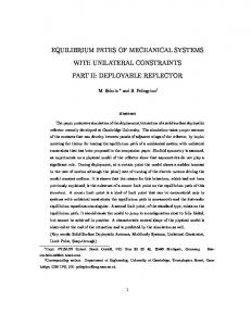
Five bridges (two composite steel girder, two pre-stressed voided slab, and one composite prestressed concrete girder) with fundamental frequencies between 4 and 10 Hz were tested with various iterations of the system. Between three and six modal frequencies and mode shapes were measured for each structure. The first six modes and frequencies for the composite pre-stressed concrete girder bridge were within 3 percent of results measured by the Targeted Hits for Modal Parameter Estimation and Rating (THMPER™) system, which is deployed in support of the Federal Highway Administration’s Long-Term Bridge Performance Program.
Fundamental Frequency (Hz)
18.0 16.0 14.0 12.0 10.0
Washburn Way, 10
8.0
Wall St., 7.8
6.0
Harbor Isles Blvd., 4.55 Eberlein St., 4
4.0
I84 WB, 4.5
2.0 0.0 0
50
100
150
200
250
300
Span (ft)
While other excitation methods (ambient traffic and impact) were considered as well as other response measurement methods (vision sensing), the shaker and iPod system was determined to be robust, forgiving, accurate, and relatively easy to use. Improvements to be considered in future work include a more rigorous frequency identification step, a denser sensor array during the confirmation step, and greater consideration of the modeling and model updating steps, all to support more accurate determination of mode shapes. As a result of this work, the RDSETGO system is sufficiently developed to incorporate additional refinements, to support a more systematic study of bridge dynamic performance, and to be considered for regular deployment by bridge inspection personnel.
2
1.0
INTRODUCTION
Bridge assessment and asset management represents a significant cost and effort to support the safety of the nation’s transportation network. Methods of bridge condition evaluation, as outlined in the National Bridge Inspection Standards, are updated regularly to reflect current knowledge of failure mechanisms in bridges. Bridge load rating methods, as outlined in the AASHTO Manual for Bridge Evaluation, are also maintained to ensure that failure mechanisms that limit a structure’s capacity are used to practically evaluate the structure and prevent unsafe loads from crossing. Condition and load ratings represent the most significant factors in a bridge’s sufficiency rating, the primary metric used to prioritize structural rehabilitation and replacement activities nationally. The accuracy of each of these activities is important given (a) the money, time, and effort expended to conduct them, (b) the decisions that are made with the information generated, and (c) the potential impact to interstate commerce and public health, safety, and welfare. While many elements of our nation’s critical infrastructure are evaluated and maintained regularly, the nation’s bridge inventory system represents one of the most robust, effective, and widespread efforts to align the efforts of engineers in departments of transportation in every state and municipality. Leveraging the latest technological advances, science, and practical knowledge is critical to maintaining our nation’s infrastructure. Dynamic testing and modal analysis of bridges have been identified to be valuable methods of conducting refined condition and load rating of bridges, and there are many researchers and participating departments of transportation who are interested in employing these methods in the field. The primary challenges in the implementation of such systems have been driving down capital and per-test time and cost, making equipment easily and quickly field deployable, ensuring that measurements are accurate, and that the system is capable of being used effectively by bridge inspectors. This report will 1. describe the problem of conducting modal testing to support bridge condition and load rating, 2. provide background on the methods available as well as those considered in this study, 3. describe the approach taken to develop the RDSETGO system, 4. describe the system developed to address the challenges of field testing bridges to determine modal properties, 5. provide findings from laboratory testing of system components and field testing five steel and concrete bridges in Oregon with various iterations of the system, 6. offer conclusions from both the development and use of the system, and 7. offer recommendations for future use and development of the system.
3
There are two purposes of a system like this: 1. Damage detection: to provide a basis for identifying or evaluating damage sustained in a significant loading event like an earthquake or bridge strike. 2. Model validation: to validate a structural model for use in refined condition and load rating. The following sections will elaborate on the specific challenges in developing a modal testing system.
1.1
PROBLEM
Bridge modal testing to support bridge condition and load rating has been pursued since the 1960s with single-input single-output (SISO), single-input multiple-output (SIMO), multipleinput multiple-output (MIMO), and output-only methods identified for potential use, each with their own strengths and drawbacks (Aktan et al., 2005). In addition to the experimental methods, post-processing methods that yield actionable data have been developed with the ultimate goal of more accurately quantifying structural condition (aka health). This report focuses on the development of a modal testing system for bridges capable of generating global dynamic system parameters. Further use of these results to draw conclusions about structural health or identify local damage was only studied insofar as it would influence the results produced by the system. The ideal qualities of the system were that it be 1. Portable and easily deployable; compact with components capable of being deployed by a bridge inspection crew or single crewperson with little prior training in structural dynamics. 2. Economical; low capital cost and per-test costs, in terms of deployment time and impact to the transportation network. 3. Accurate; results should be repeatable and representative of the structure tested. A rigorous evaluation of system qualities could be conducted by considering the framework of Aktan et al., which is depicted in Figure 1.1. While many of the items in this framework were considered, they were not measured at every iteration of the system. Rather, RDSETGO was developed primarily with the structure and the tester in mind. Put simply, Aktan et al. emphasize that “the dynamic test of a constructed system should therefore be executed with a careful evaluation of observability, repeatability and the system of interacting elements of the engineered structure, the nature and the human.” Indeed, this was the case in the development of RDSETGO. The system was continuously refined based on evaluation of its challenges in each iteration.
4
Figure 1.1: SHM system considerations (Aktan et al., 2005).
1.2
BACKGROUND
To understand modal testing of road and highway bridges and its real-world applications, one must be versed in a variety of areas including 1. 2. 3. 4. 5.
structural mechanics structural dynamics digital signal processing bridge condition and load rating bridge modal testing to support refined condition and load rating
This section of the report will provide background in each of these areas sufficient to understand the results presented later in the report. It will also provide background on two recent methods of modal testing and compare them to the RDSETGO system developed in this study. 1.2.1
Structural Mechanics
Structural mechanics is a field of study that relates loads and fundamental physical parameters like materials, geometry, support constraints, member connectivity, and member arrangement to the internal and external response of a structure: quantities like stresses, strains, deformations, and displacements of parts of the structure. Structural mechanics forms the basis for 5
understanding the capacity of structures to transfer and support a variety of loads (gravity, lateral, thermal, environmental, dynamic), to maintain or limit displacement of their original shape under these loads, and ultimately to perform as expected. Structural mechanics principles form the basis for additional study of structural analysis and design methods, structural dynamics, and the physical response of solids and structures at a variety of scales from the nanoscale to the largest structures on or of the earth. 1.2.2
Structural Dynamics
Structural dynamics is a subfield of structural mechanics that relates time-dependent loads to the internal and external response of a structure. While structural mechanics forms the basis for many of the necessary relationships, the study of physical behaviors that change in the time domain requires a fundamental knowledge of dynamics: relationships of position, velocity, acceleration of particles and continua. Further, the behavior of systems that do not move through space, but rather have some part fixed in space, leads to study in the field of vibrations. The fundamentals of vibrations are contained in numerous texts (Chopra’s Dynamics of Structures (2012) and Meirovitch’s Fundamentals of Vibrations (2001) are excellent sources) and will be briefly summarized in the following subsections. 1.2.2.1
Single-Degree-of-Freedom Model
Degrees of freedom are the permissible displacements and rotations of a point in space. A simple structure may often be idealized as a single-degree-of-freedom (SDOF) structure, with a lumped mass capable of displacement in a single direction, restrained by a linear spring and viscous damper, as shown in Figure 1. To calculate the undamped rotational natural frequency of such a simple system the following equation is used: ω𝑛𝑛 = �
𝑘𝑘 𝑚𝑚
(1-1)
where ωn is the rotational natural frequency in rad/s, k is the stiffness in lb/in, and m is the mass in lb-s2/in. As there is only one degree of freedom, there is also only one mode shape, a displaced one, hence the simplicity of the equation. The natural frequency can be related to the cyclic natural frequency, fn, and natural period, Tn, using the following equation: 𝑇𝑇𝑛𝑛 =
1 2(𝜋𝜋) = 𝑓𝑓𝑛𝑛 ω𝑛𝑛
(1-2)
where Τn is the natural period in sec and fn is the cyclic natural frequency in Hz or cycles per second. The natural period of a structure is the amount of time it takes to go through a full cycle of displacement. The higher the frequency the shorter the period, as they are inversely proportional.
6
Figure 1.2: A lumped mass roller, used to model a single degree-of-freedom structure (Chopra, 2012).
1.2.2.2
Multi-Degree-of-Freedom Model
A multi-degree-of-freedom (MDOF) structure allows for consideration of more than one direction or rotation at any one time, so more detailed structural deformation can be considered. Matrices are used to contain lumped mass quantities, as well as the stiffness and damping quantities of connecting elements of the structure. The number of fundamental mode shapes and natural frequencies is equal to the number of degrees of freedom of the system. An example of a MDOF structure is a tower with lumped masses at each floor. For structures like these, the participation of each mode can be represented by the effective modal mass and modal height on the right of the figure. These two properties can be used to represent each mode as that of a SDOF system, shown in Figure 1.3, and they represent the relative strength of a modal response. One can envision the relative ease of measuring the response of the “larger” lower-frequency system represented in mode 1 versus the “smaller” higher-frequency system in mode 5. This will become apparent later as lower-precision tools, like iPod accelerometers, are able to measure accelerations of lower modes but not necessarily of the highest ones.
Figure 1.3: A MDOF system with effective SDOF modal models (Chopra, 2012).
7
1.2.2.3
Continuous Model
Single- and multiple-degree-of-freedom models are ultimately simplifications of continuous structures. A continuous model, such as the simple beam shown in Figure 1.4, has a uniformly distributed mass and stiffness and is analogous to a guitar string. The natural frequencies for the simply-supported continuous beam in Figure 1.4 can be calculated using equation 1-3: 𝑛𝑛2 𝜋𝜋 2 𝐸𝐸𝐸𝐸 ω𝑛𝑛 = 2 � 𝐿𝐿 𝑚𝑚
(1-3)
where L is the length of the span, E is the modulus of elasticity, I is the moment of inertia, m is the mass per length, and n is the mode number, an integer value greater than zero. The mode shape that corresponds to the nth natural frequency can be calculated using equation 1-4: 𝑛𝑛𝑛𝑛𝑛𝑛 � 𝐿𝐿
φ𝑛𝑛 (𝑥𝑥) = 𝑠𝑠𝑖𝑖𝑛𝑛 �
(1-4)
Figure 1.4: Continuous beam with three mode shapes - each mode shape adds another node, or zero displacement location, and another half wave along the length of the beam.
Continuous structures, like bridges, cause several difficulties when modeling and determining the natural frequencies, given their complex distribution of mass, stiffness, and variable-stiffness supports. These challenges will be discussed further in the next section. 1.2.2.4
Difficulties Modeling Continuous Structures
The difficulties associated with continuous structures have to do with the relative complexity and the challenge of describing the structure’s stiffness and mass distribution in closed form such that a closed form solution can be determined. Because this is only possible for a few relatively simple plate and beam systems with well-described constraints, approximate MDOF structural models are often used. As the stiffness and mass of the structure are distributed it requires a good understanding of how these variables change along the length of the structure to discretize the 8
model. Additionally, there are components of a bridge that affect the stiffness, such as railings, that are not commonly assumed to be structural but nonetheless affect stiffness quantities that impact dynamic response. This means that a bridge model needs to take into account the entirety of the bridge by modeling stiffness contributions of both structural and non-structural components. When modeling a bridge, it can be shown that the boundary conditions have a direct effect on the response and natural frequency of the structure. This is particularly hard to model, as most bridge structures use some component of the surrounding soil to support the structure, whether it is in uniform bearing or otherwise. The interaction between the structure and the soil is difficult to model and can add substantial complexity to a model. In most cases, simpler support conditions are assumed. A continuous three-dimensional structure has more than just vertical modes. Lateral and torsional modes of vibration should also be considered. When data is recorded on only one side of the structure it is difficult to determine whether the mode shape of the bridge is purely vertical or if there is a torsional component. By increasing the resolution of accelerometers across the bridge, it allows for more of these additional mode shapes to be identified and differentiated. During the testing of a bridge, using either free or harmonically forced vibrations, explained in Section 1.2.2.5, the interaction of traffic can influence response measurements. It is necessary to have a limited amount of traffic crossing the bridge to decrease the effective noise in the system. This can become increasingly difficult without the use of lane or bridge closures when the structure is heavily trafficked. However, harmonically forced vibration testing creates a continuous excitation and resonant response that can often be identified regardless of changes in ambient excitations.
1.2.2.5
Free and Harmonically Forced Vibration
The natural frequency and mode shapes of a bridge can be determined using both free and harmonically forced vibrations. Free vibration response can be measured by applying a single impact load on the structure and allowing the structure’s vibrations to damp naturally. Harmonically forced vibration testing supplies a consistent harmonic forcing at a specific frequency that can excite or resonate natural frequencies in the structure. A structure experiencing free vibrations receives an initial impact which has a distinct frequency range but can excite many modes of vibration at different frequencies. A similar response can occur when a large vehicle crosses a bridge; however, live traffic tends to cause large numbers of frequencies with a more uniform frequency distribution. Regardless of excitation, a response frequency which has a larger amplitude, and has a stronger presence, is more likely to be a natural frequency. The response of a structure is very different when the structure is harmonically forced. When a structure is harmonically forced at a natural frequency (typically called resonance), the structural response is dominated by that natural frequency. This allows for a more accurate 9
determination of a natural frequency because the response of a system is amplified and therefore easier to measure. However, it is necessary to determine what these natural frequencies are before resonance testing, say by testing the structure in free vibration or by monitoring ambient vibration response for candidate natural frequencies. It is also possible to find natural frequencies by systematic harmonic forcing of the structure using a sweep of frequencies from low to high to identify those frequencies at which a more significant response occurs. In any case, the locations of the forcing and response measurement are important and are ideally at the so-called anti-nodes of the response, the location where response is maximum. Theories of structural dynamics have been well studied, with research continuing to this day. This section only seeks to provide basic background on the study of vibrations, as other literature is available for further information regarding this topic. It should be noted here that medium- to long-span highway bridges have a common frequency range of 2-4 Hz and damping ratios of less than 2 percent (Bachmann et al., 2012). A simple estimate of the first natural frequency, based on a study of 224 highway bridges, is provided by Cantieni (1984): (1-5) 𝑓𝑓 = 100/𝐿𝐿 where f is the natural frequency in Hz and L is the longest span length in m. 1.2.3
Digital Signal Processing
Digital signal processing is a critical component of any vibration testing. Many references are available that provide the fundamentals of signal processing (e.g., Kahn, 2005). The most practical tool for working between the time and frequency domains is the Fast Fourier Transform (FFT), which operates on a signal in the time domain (acceleration vs. time in this case) to produce the power spectral density (PSD) of frequencies in the signal. With this functionality programmed into a suitable app on an iPod or other mobile device, the number of postprocessing steps in vibration testing is vastly reduced and data in the time domain need not be analyzed offsite. This provides a distinct advantage for iPods in the vibration testing environment. One challenge of this method, however, is that unsynced iPods producing frequency response directly do not provide the ability to determine phase differences between sensors at various locations in the structure. Each sensor effectively produces an absolute value of acceleration amplitude and frequency. Thus, a first torsional and first flexural mode measured at the edges of a structure may appear the same and can only be distinguished by measuring values in the interior of the structure. This challenge and methods to overcome it will be addressed further in the Findings and Conclusions sections of this report. Other improvements that remain to be incorporated into existing apps include control of time windows, sample rates, and application of filters directly within mobile apps. Some apps have these features and are discussed in more detail in the Development of Response Measurement System section of this report.
10
1.2.4
Bridge Condition and Load Rating
Bridge condition and load rating procedures are described in the AASHTO Manual for Bridge Evaluation (2016) and are adopted, sometimes with modification, by the Federal Highway Administration (FHWA) and state departments of transportation. Bridge condition ratings exist on a scale from 0 to 9 and are based on the results of a detailed element-level bridge inspection, which may include visual and non-destructive techniques. The components of a bridge that are rated include the deck (driving surface and structure carrying wheel loads to the superstructure elements); the superstructure (the primary load carrying elements, commonly girders, that transfer deck loads to the substructural elements); and the substructure (the components supporting the superstructure that include abutments and piers, which carry loads into the ground). Condition rating codes, descriptions, and commonly employed feasible actions from the FHWA Bridge Preservation Guide are included in Table 1.1.
Table 1.1: Condition rating codes, descriptions, and commonly employed feasible actions (FHWA, 2011)
The impact of bridge condition ratings on bridge load ratings is dictated by the AASHTO Manual for Bridge Evaluation in the condition factor, φc. Bridges with a condition rating of 6 (good) or higher require no reduction in capacity due to condition. However, those with a condition rating of 5 (fair) or 4 (poor) for the element controlling a load rating take an additional reduction in the element capacity based on that condition: 5 percent reduction for fair condition, 11
15 percent reduction for poor condition. In addition, detailed measurements of section loss can be incorporated into a load rating calculation. However, it is this relatively crude approach that systems like that explored in this report can help to improve. If more precise measurement of condition is possible, then more accurate reductions in structural capacity can be used, resulting in a more accurate load rating.
1.2.5
Bridge Modal Testing to Support Refined Condition and Load Rating
This section describes the RDSETGO system in summary as well as two different dynamic testing systems deployed by two different research groups: Islam et al. (2012) at Youngstown State University and Moon, DeVitis and others at Drexel and Rutgers (2015). Each of these studies will be summarized and compared to RDSETGO. 1.2.5.1
RDSETGO System Summary
The development of the RDSETGO system is described in the Approach section, while the current, most developed version of the system, as well as its deployment procedure, is described in the Methodology section. The remainder of this section will provide a brief summary of the system as context for the comparisons to other systems. The RDSETGO system consists of components that allow for harmonic forcing of a structure via an electromechanical shaker and response measurement with an array of iPods: Excitation: APS Electroseis™ 113 shaker with 15-pound inertial weight Response Measurement: 12 third-generation iPod Touch units running the VibSensor and Vibration Analysis apps Data Collection: Visual/manual reading and recording of amplitude and frequency Post-processing: Excel for x-y scatter plotting, Matlab for interpolated mode shape surface/contour plots Structural modeling: MIDAS Civil (3D FEM) or MASTAN2 (1D and 2D modal analysis) The procedure for using the system in summary is: 1. A priori model or mode shape estimation to identify likely antinode locations and possible mode shapes and modal frequencies. 2. Ambient vibration or periodic impact testing with a single iPod placed at all likely antinodes. 3. Forced vibration testing with the shaker placed at antinode locations and iPods at locations on the structure sufficient to confirm mode shape. 4. Data collection for all possible mode shapes and frequencies. 5. Data post-processing and visualization. 6. Model adjustment. The goal of the system is to support bridge asset management via refined condition rating, structural evaluation after a significant loading event such as the Cascadia Subduction Zone earthquake, or damage detection based on periodic structural evaluation. 12
Many other efforts to develop and deploy bridge vibration measurement and experimental modal analysis systems exist. Two recent examples that will be described in the following sections are: 1. A controlled live load procedure employing a wireless accelerometer sensor network developed by researchers at Youngstown State University and supported by the Ohio DOT (Islam et al., 2014). 2. The Targeted Hits for Modal Parameter Estimation and Rating (THMPER™) system developed at Drexel and Rutgers by a team led by Frank Moon, which employs a single drop-mass impulse at multiple locations and an accelerometer sensor network to characterize the dynamic properties of a structure (DeVitis, 2015). 1.2.5.2
Ohio DOT Research Summary
The Ohio DOT has been looking for a way to measure and provide meaningful data from the dynamic response of a bridge for condition assessments and load ratings. In 2012, ODOT supported Youngstown State University researchers Dr. Anwarul Islam and Dr. Frank Li in creating a system of wireless sensors to compare field results with the dynamic response of a modeled bridge, using Finite Element (FE) Analysis. To properly validate and apply the findings of the research, Islam et al. selected new and old bridges. The selection of older bridges ensured that the data collected included structures with a degradation in structural capacity. The process of validating an FE model with the newer bridge allows for clear determinations of how the older structures should compare. 1.2.5.2.1 Field Investigations Using a base station connected to a laptop, Sun Small Programmable Object Technology (SunSPOT) sensors collected real-time acceleration data during the field investigations. The SunSPOT sensors allowed for data concerning temperature, amount of light, and acceleration response to be recorded. Recording only the z-axis (vertical) acceleration of the tested bridge, the sensors measured three separate trucks as they traversed the test bridge. Dump trucks were selected to be the vehicles to traverse the centerline of the selected bridges. Three truck weights (empty, half-loaded, and full) were selected to observe the change in amplitude and vibration of the structure due to the varying weights. The dump trucks drove down the longitudinal centerline of the bridge, with the SunSPOT sensors located 2 feet to one side. The acceleration response of the bridge with the dump trucks traveling along the designated path was recorded for use in the analysis phase of the project. The transformation of the acceleration versus time data into acceleration versus frequency was performed using the FFT technique. This allowed for possible natural frequencies of the structure to be determined. Frequencies along the acceleration versus frequency graphs that have the highest amplitude are more likely to be the natural frequency for a mode shape, as the bridge is naturally trying to vibrate at these frequencies.
13
1.2.5.2.2 FEA Modeling The purpose of creating an accurate model of the existing bridges in as-designed condition is to allow for a good understanding of the condition and load rating of the bridge, as they currently exist compared to an estimated as-built condition. To create an accurate model, five separate parts were modeled individually. These parts consisted of the following, with associated material: 1. 2. 3. 4. 5.
Wearing Surface – Asphalt Concrete Prestressed Concrete Box Beam – Prestressed Concrete Reinforcing Steel – Steel Prestressing Strands – Steel Meshed FE Bridge – Various
Upon creation of each part of the FE model, an interaction module was updated to manage how each of these parts would interact. Once the final FE model had been completed, loads could be applied. Load generation was done using the VDLOAD subroutine, written in Fortran, in which the varying dump truck loads were applied to the bridge at varying speeds. The weights for each dump truck wheel were assumed to act uniformly under the contact area, as a point load, and sensors were placed in the model at the same locations as on the test bridge. Once loads were applied, the researchers could model the static and dynamic properties of the model structure. 1.2.5.2.3 FEA Validation The validation of the FE model consisted of comparing the results to field tests and theoretically. The FE model produced a natural frequency of 3.55 Hz, while the field testing indicated a natural frequency of 3.44 Hz, a difference of 3.1 percent. The theoretical method also produced similar results as the FE model through the use of theoretical hand methods to calculate the natural frequency of the bridge. Islam et al. idealized the bridge as a beam with two fixed ends. These hand calculations produced a natural frequency for the first mode of 3.44 Hz, which is the same as the field testing. 1.2.5.2.4 Fundamental Frequency Analysis As a bridge ages and its capacity decreases, it is unlikely that a significant loss of mass will occur. Since a simulation of the damping mechanism of this structure was outside the scope of the study, this allows for a narrowing of possible reasons for the decrease in natural frequency. Since two of the three factors in determining natural frequency and the response of a structure (mass, stiffness, and damping) have been removed from consideration, a change in stiffness could be attributed to the change in response. Stiffness is dependent on material stiffness (modulus of elasticity), geometric stiffness (moment of inertia) and support conditions. Research has demonstrated that material stiffness is relatively stable in time and the support conditions have not changed with time. Therefore, it is most likely that the structure has experienced a change in geometric stiffness throughout the life span of the bridge.
14
1.2.5.2.5 Condition and Load Rating Islam et al. (2014) suggest that the difference in natural frequency between a modeled and tested structure can be attributed to a reduction in section properties, a conservative assumption that can then be applied to a change in condition and load rating. Upon modeling and testing of an older bridge with the validated FE model, with a Modal Assurance Criterion (MAC) analysis showing a correlation of 71 percent to 86 percent, the change in condition rating could be determined. Assuming that the bridge was built correctly, the FE model outputted a natural frequency of 5.45 Hz. This frequency varies from the field-tested bridge by 36.9 percent, at 3.44 Hz. Islam et al. took the 36.9 percent change in natural frequency and correlated this change in natural frequency to a change in the initial superstructure condition rating of “9,” or a bridge in excellent condition. ODOT rated the existing superstructure a “6”, a three-point loss from when the bridge was first constructed. A superstructure with a condition of “6” is in satisfactory condition and shows minor deterioration, additionally in the AASTHO Manual for Bridge Evaluation this rating requires the application of a 0.95 factor to be applied to the capacity. Islam et al. determined that a 36.9 percent change in natural frequency correlates to a three-point decrease in condition rating. Similarly, it was found that the load rating of the bridge, using the FE model, was similar to ODOT’s findings. The FE model produced a load rating of 4.147 for a 16-ton vehicle (OH-2F1), while ODOT determined it to be 4.708 and 4.867 using VIRTIS and BARS, respectively. These close similarities make this research method valuable and implementable. It is important to note that even though the FE model used was validated, shown previously in Section 1.3.2.3, the method to create the model was not validated. In the initial methodology of the Islam et al. study, it was decided that four bridges would be condition rated and would undergo testing. The purpose of this was to gather field data and build FE models for two deteriorated bridges and two relatively new bridges. Due to unforeseen circumstances, the sensors were destroyed on one bridge and were not fully attached to the other; only one bridge that had experienced deterioration was tested. This meant that a FE model using the method described above could not be confirmed to truly model an existing new bridge. It is possible that errors exist in the model, which account for the difference between the FE model load rating and the ODOT load rating. It is also possible that these same errors can attribute to the difference in the fundamental frequency. Ultimately, the true source of the difference remains uncertain. 1.2.5.2.6
Ohio DOT vs. RDSETGO
RDSETGO and the Islam et al. methods for determining natural frequencies of an existing structure have several key differences in how the bridges are forced, data is collected, and the structure is modeled. These differences indicate both benefits and challenges for each of the methods. The following sections will describe the differences between the excitation, data collection, and modeling aspects of each method. 1.2.5.2.6.1.Excitation Method Both the RDSETGO and Islam et al. methods implemented field testing to determine the existing structure’s natural frequency. To obtain the natural and fundamental frequencies of a particular 15
bridge, Islam et al. used dump trucks with three different loads driven down the center line of the bridge (2014). RDSETGO, however, uses a shaker system which can be placed at varying locations along the span of the bridge. This system allows for specific frequencies and modes to be forced on the bridge, resulting in a more reliable forcing of specific mode shapes. Data collection between the two methods also varied. 1.2.5.2.6.2.Data Collection To record the structure’s vibrational response with respect to both frequency and amplitude, the RDSETGO method uses a system of 12 iPods. Each of the iPods is evenly spaced along the span of the bridge and is merely placed on the structure rather than affixed with adhesive or fasteners. Data is collected by manually reading each iPod. As discussed in Section 1.3.2.1, Islam et al. used a similar method of sensors connected through a network reporting data to a controller. While the collection of data is streamlined and phase can be interpreted, the setup for the Islam et al. method required that the sensors be next to moving vehicles and firmly affixed. Since RDSETGO allows for simple contact of the iPods, it can be quickly set up and taken down. The Islam et al. method of data collection does have a major benefit over the RDSETGO method. By having the data collectors attached to a network, recorded data can be easily viewed on a computer on site. RDSETGO, however, requires an individual to read each of the iPods individually. This allows for possible errors to occur, and adds time to the data collection process. Data transmission from the iPods has been reserved for future development. 1.2.5.2.6.3. Structural Modeling Both the RDSETGO and Islam et al. methods have a step where the existing bridge is modeled to determine the natural frequency. Islam et al., created a FE model focusing on four separate parts of the structure. This is done to compare the existing structure with the model to determine if any degradation has occurred. RDSETGO, on the other hand, uses MIDAS Civil software to model the existing bridge. The purpose of this modeling in RDSETGO is to serve as an a priori model to estimate natural frequencies and mode shapes, primarily to determine the locations of antinodes that will be forcing locations in the field. Direct comparison of the modeled and tested structures are not intended to be used to draw conclusions about deterioration of the structure without further study. Attributing model differences directly to stiffness reductions, while conservative, is imprecise. Rather, differences in tested values between visits to a structure are intended to be used for this purpose in the RDSETGO system. 1.2.5.3
Targeted Hits to Measure Performance Responses Summary
The THMPER™ system is a method developed by John Devitis et al., and was documented in Devitis’s dissertation in 2016: “Design, Development, and Validation of a Rapid Modal Testing System for the Efficient Structural Identification of Highway Bridges.” Similar to the Islam et al. and RDSETGO methods, THMPER™ uses modal testing to determine global performance of a bridge and to specifically compare to pre-existing static load testing methods. This section will summarize the work done by Devitis et al. and the method devised. 16
1.2.5.3.1
THMPER™ System
The THMPER™ system consists of a modal testing trailer that can be attached to a towing vehicle with a mobile workstation. A hammer capable of generating forces of more than 25 kips in a frequency range of 0 Hz to 50 Hz (the frequency range in which the many modes of vibration are usually found highway bridges) is attached to the back of the trailer. A mobile sensing array is used to record data for 10 seconds at a sampling rate of 3,200 Hz. This array also turns on pneumatic actuators to stop the rebounding of the hammer, allowing for a unit impulse and a preservation of data quality. Additionally, two mobile sensing systems are used on both sidewalks of the structure to allow for spatial sensing and modal references. These mobile sensing systems consist of accelerometers whose data are recorded by a GPS synchronizing system. This system is wireless and sends the recorded data to a central point on the modal testing trailer, to be collected and sent to the mobile workstation. The purpose of these sensors is to provide both modal and spatial references for the collected data, and to ensure that the correct mode shapes are identified. 1.2.5.3.2 Test Methodology It is common in structural dynamics to create a Frequency Response Function (FRF), a quotient of the output and input frequency spectra, which can be used to identify and quantify resonances and damping parameters. In the case of THMPER™, the y-axis of the FRF is the amplitude and the x-axis is the frequency. When looking at an FRF graph, the natural frequencies are identifiable as peaks in the graph. The width of the peaks is a measure of the damping of the structure; in essence, a structure with wider peaks will have a stronger damping than one with narrow peaks. When the FRF is produced for sensors at various locations in a well-synced system, the phase of the vibration and the peak frequencies can be used to identify mode shapes. Once Devitis et al. obtain acceleration response data from their sensor network, they process it via a proprietary software that automatically checks data quality (data points that appear to be noise, dropped channels, overloading of the load cells, and proper time synchronization). The final data output can then be analyzed and processed via custom software. The software develops a FRF and, after more data management, an Enhanced Frequency Response Function (eFRF) is produced. Each peak of the eFRF is a natural frequency associated with a mode shape. To show the efficiency of this particular method, Devitis et al. performed testing in this 2016 study on the Pennsauken Creek Bridge, located in New Jersey. 1.2.5.3.3
Pennsauken Creek Bridge Case Study
To demonstrate that the THMPER™ method was a valid alternative to other traditional methods of dynamic testing, like MIMO, Devitis et al. performed testing on the Pennsauken Creek Bridge. This bridge consisted of three continuous 50-foot spans made of hot-rolled steel with a concrete deck. To ensure sufficient resolution to construct mode shapes, a total of 28 accelerometers were placed on the bridge. Devitis et al. determined that five impact locations would be used for both testing methods, dynamic and static, aimed at producing the highest 17
amplitude of vibration. The static testing was conducted using a 086D50 model instrumented sledge hammer. The 086D50 can apply a force of zero to five kips with a weight of 12.1 pounds.
Upon completion of the testing, during the analysis of the data, a partial modal parameter comparison was made. The purpose of this was to compare the current static standard sledge using MIMO impact testing and the THMPER™ single-input-multiple-output (SIMO) method. The resulting frequencies found with both of these methods were found to be relatively similar. Mode one for the bridge was found to be at a frequency of 7.39Hz using THMPER™ and 7.47 Hz using the 086D50 sledge, a 1.07 percent difference. This difference, however, does not show the major benefit of the THMPER™ system over the conventional method. The bridge’s vibrational amplitudes between the two methods is significantly different. THMPER™ was able to excite the bridge at roughly 2 g, while the standard sledge only excites a maximum amplitude of 0.5 g. This increase in amplitude was clear in the graphical representations of the mode shapes. Additionally, this increase in amplitude allows for sensors which do not need to be able to record small amplitudes with a great amount of accuracy, allowing for a less expensive measurement system. 1.2.5.3.4
THMPER™ vs. RDSETGO
The THMPER™ and RDSETGO methods share similar attributes and are both looking for ways to create a method in which DOTs can dynamically test a bridge in a cheap and effective manner. This section reports the similarities and differences between THMPER™ and RDSETGO. 1.2.5.3.4.1.Excitation Method Both the THMPER™ and RDSETGO methods use a measured-input excitation. THMPER™ does this by applying a single impact, and recording the bridge response, applying another load in a different location once the bridge has damped out. Due to the frequency range that the weight can excite from the bridge, THMPER™ is best for finding the fundamental frequencies of a bridge in a range usually from 0-50 Hz, very precisely. RDSETGO applies a harmonic forcing frequency, using a shaker on the bridge, and resonates the bridge at the natural frequency for each mode to allow sufficient time for data collection. Resonance testing takes advantage of dynamic amplification, so the RDSETGO system can be much smaller. However, the energy imparted to the structure by the relatively small shaker is substantially less than that of THMPER™’s impact system. While substantial enough to generate accelerations measurable by iPod, higher modes can be lost by the RDSETGO system while THMPER™ can identify them precisely. Since RDSETGO’s shaker system is smaller and lighter than the THMPER™ method’s modal testing trailer, it does not require a lane or bridge closure to complete testing. The THMPER™ system requires for at least a single lane to be slowed, as the trailer is attached to a mobile work van. During the I-84 WB bridge test, the RDSETGO system was successfully tested in the shoulder of a three-span continuous bridge. The natural frequencies associated with the first six modes were found at the barrier and fog line and extrapolated to accurately differentiate these
18
mode shapes. A detailed comparison of THMPER™ and RDSETGO results is provided in the Findings section. 1.2.5.3.4.2.Data Collection THMPER™ collects data in three locations using accelerometers on the modal testing trailer and on either the sidewalks or shoulders of the bridge. This is done to measure structural response and to identify the mode shape. Using a wireless accelerometer network, data can be sent to a centralized location, similar in practice to the Islam et al. method. The RDSETGO method takes advantage of an inexpensive and widely available iPod system at the expense of rapid data collection. However, wireless data collection may be developed in the future. The footprint of THMPER™ is physically bigger and requires a trailer. This shows the major benefit of the RDSETGO method, in which all of the equipment can be carried in two large plastic totes. Additionally, the smaller form factor of the RDSETGO hardware allows for a shorter setup time and shoulder-only deployment. This is not to say that RDSETGO could not improve to assimilate some of the proven benefits of the THMPER™ method. The major benefits of THMPER™ over RDSETGO are precision and processing speed. The sensors can directly relay data to a central location, speeding the data collection and processing steps. The ability to conduct testing without having to put personnel on an active travel way is a major benefit that allows for a comfortable and safe work environment. 1.2.5.3.4.3.Data Processing After acquisition of data, the THMPER™ method processes the data with custom software that vets the data and ensures accuracy. Once the data has been checked by the software it is then analyzed and graphed. The RDSETGO method is more manual at this point in its development, and requires a person to transfer the manually collected data to Excel and Matlab for visualization. Since THMPER™ wirelessly transfers data to a single workstation, vetting of the data by software is much more streamlined. However, the mode shapes and frequencies determined by the two systems have been found to be within 3 percent. 1.2.5.3.4.4.Structural Modeling To create a structural model for comparison, Devitis et al. created an FE model using the RAMPS software, a custom program made at Drexel University. Following the completion of the model, modal analysis was compared to both the THMPER™ testing and sledge testing and the model was modified until the results converged. The purpose of this was to find the inventory and operating load ratings each method produced for the bridge being inspected and for an HL93 truck. RDSETGO currently uses MIDAS Civil software to create a detailed 3D model of the bridge in question. This software is relatively common in the bridge design industry and is licensed by the Oregon DOT for detailed structural modeling purposes. 19
It is important to note that the RAMPS software has been demonstrated in the testing of the THMPER™ system to produce accurate load ratings. This level of development has not been achieved in the RDSETGO system. Further work is necessary to show that the RDSETGO method can produce an accurate load rating using the MIDAS Civil software.
20
2.0
APPROACH
The RDSETGO system was prototyped and revised multiple times to achieve the performance goals (Table 3.1). The bulk of the work was in the excitation and response measurement components of the system. The remainder of this section will describe the evolution of the system in each iteration. The current version of the system will be described in detail in the Methodology section. Table 2.1: RDSETGO system development iterations Response Power Excitation measurement Iteration supply system system 1
2
3
Generator
300-lb shaker frame with APS Electroseis™ 113
Generator
300-lb shaker frame with APS Electroseis™ 113
Generator
4
Generator
Future
2,000W power inverter in support vehicle
2.1
iPhones running Vibration Analysis app
APS Electroseis™ 113 shaker with 10-lb additional weight APS Electroseis™ 113 shaker with 10-lb additional weight
12 3rd generation iPods running Vibration Analysis app 12 3rd generation iPods running Vibration Analysis app 12 3rd generation iPods running Vibration Analysis app
APS Electroseis™ 113 shaker with 10-lb additional weight
12 3rd generation iPods running Vibration Analysis app
Transportation system
Quantities measured
24-ft enclosed trailer and hauling vehicle, pallet jack
Modal frequencies
4’x8’ utility trailer and small hauling vehicle 3.5’x4’ utility trailer and small hauling vehicle 2 30-gallon Husky storage totes and small SUV or minivan 2 30-gallon Husky storage totes and small SUV or minivan
Modal frequencies, mode shapes
Modal frequencies, mode shapes, modal damping ratios Modal frequencies, mode shapes, modal damping ratios Modal frequencies, mode shapes, modal damping ratios
DEVELOPMENT OF THE EXCITATION SYSTEM
Excitations can be classified as either ambient or measured-input (Farrar et al., 1999). Ambient excitations (associated with so-called operational modal analysis) are those that occur during the normal service conditions for a structure, including vibrations induced by wind or live loads. Ambient excitations often have a frequency spectrum that is uniform or can be classified as noise, but some excitations like seismic loadings have a dominant frequency or frequency band. Ambient excitations are valuable for simple output-only response measurement methods because the quality of the input is variable and need not be quantified. Measured-input excitations like drop-mass and forced harmonic vibration (associated with so-called experimental modal analysis) are more valuable in modal testing because the controlled input and testing protocol and carefully measured output provide the most deliberate control and reproducibility of the input signal. 21
2.1.1 Periodic Impact Prototypes 2.1.1.1
Ambient Traffic
Ambient traffic excitation can play a valuable role for structures that have regular vehicle traffic. Some output-only modal analysis methods use this source of excitation exclusively. Our team took advantage of ambient traffic excitation in preliminary estimations of modal frequencies. These frequencies became the starting point for more deliberate forced vibration testing. 2.1.1.2
Jumping in Unison
Given its prominent role in many vibration studies, periodic jumping was used early in the system development and is a fundamental component in the preliminary estimation step. 2.1.1.3
Drop Mass Systems
Drop mass systems were considered during the course of system development. A modified Standard Penetration Test apparatus was prepared but ultimately deemed unsafe for field deployment without further refinement, which was not pursued.
2.1.2 Harmonic Oscillation Prototypes Each of the harmonic oscillation prototypes took advantage of the APS 113 Electroseis™ shaker. Other inexpensive systems were considered, like plate compactors, modified jack hammers, and eccentric mass vibrators, but these were ultimately not explored for a variety of reasons including cost (for eccentric mass vibrators) and perceived precision and control challenges (for plate compactors and jack hammers). Eccentric mass vibrators have been used successfully and ANCO Engineering, Inc. in Boulder, CO, markets custom systems that may be explored in the future. In the following sections, the evolution of the RDSETGO system, from one employing the shaker in free-body mode to fixed-body mode, will be described. The difference between freebody and fixed-body modes is the motion of the shaker frame; in free-body mode the relatively heavy shaker body is excited, while in fixed-body mode the relatively light armature moves while the shaker body is fixed to the structure. 2.1.2.1
Free-Body Shaker Systems
The shaker system was originally conceived to take advantage of the full shaker body weight (78 pounds) by using the shaker in free-body mode. This required development of a suspension system to support the shaker body in a neutral position, which was the work of Alexander Antonaras in his graduate project (Figures 2.1 and 2.2). Details of the development of the shaker frame are included in the graduate project report by Alex Antonaras to be published by the Oregon Institute of Technology. This system was only deployed once on the Eberlein Avenue bridge. At this point, the equipment required to control the shaker was still relatively disorganized and the system required a significant amount of equipment and personnel to deploy.
22
Controller
Amplifier and laptop
Shaker frame
iPods Generator Figure 2.1: RDSETGO Iteration 1 with heavy shaker frame.
Figure 2.2: Description of heavy shaker frame in RDSETGO Iteration 1.
23
Ultimately, the shaker frame was considered to be too heavy and challenging to move. In order to improve portability, the frame was incorporated into a 4’x8’ utility trailer where it could be towed to the test location and lowered into place by a winch that was mounted on the shaker frame and supported at the apex of a tripod attached to the trailer frame (Figures 2.3 and 2.4). While this system significantly improved the portability, no longer requiring a large trailer to transport the frame and a pallet jack to move it into place, it continued to have a fairly large footprint and required the use of the heavy frame. At this point, a bridge with less traffic was identified for deployment (Harbor Isles Boulevard). After testing with the heavy frame, the shaker was removed and testing was attempted with the shaker alone. It was discovered that the 5-pound shaker armature with 10 additional pounds of weight could be supported by the heavy bands supplied with the shaker. The response of the structure to excitation by this system was nearly equivalent to that of the shaker body operating in the heavy frame. Thus, the move to a fixed-body shaker-only system was determined to be appropriate.
Figure 2.3: Elevation views of tripod-supported heavy shaker frame in RDSETGO Iteration 2.
24
iPod at each cone Amplifier, controller, and laptop
Figure 2.4: RDSETGO Iteration 2 with iPods at each cone.
A weather-proof equipment box was constructed in Iteration 2 to contain the laptop computer, amplifier, controller, and various cables required for the system (Figure 2.5). This box could also contain the shaker as the team moved to Iteration 3 with a fixed-body shaker system (Figure 2.6).
25
Figure 2.5: RDSETGO Iteration 2 with equipment box.
2.1.2.2
Fixed-Body Shaker Systems
The much smaller footprint of the fixed-body shaker system did not require the heavy shaker frame and the relatively large utility trailer to move it. This allowed the research team to further reduce the footprint of the system to a 3.5’x4’ trailer that had the potential to be moved manually along shoulders and sidewalks, possibly eliminating the requirement of a lane closure during testing (Figure 2.6).
26
Figure 2.6: RDSETGO Iteration 3 with equipment box on 3.5’x4’ trailer.
Figure 2.7: RDSETGO Iteration 3 with equipment box on carpet dolly and shaker in fixed-body mode.
27
In Iteration 4 of the system, the team dispensed with the heavy wood equipment box and distributed the computer, amplifier, control system, shaker, and cords into two 30-gallon plastic equipment totes, which could be managed by a single individual and stacked and moved around the structure as necessary on a carpet dolly. This also permitted the system to be deployed almost anywhere, including in building interiors (Figure 2.9).
Figure 2.8: RDSETGO Iteration 4 with equipment totes used to contain equipment and support a workstation.
28
Figure 2.9: RDSETGO Iteration 4 deployed in interior building walkway.
2.2
DEVELOPMENT OF THE RESPONSE MEASUREMENT SYSTEM
2.2.1 iPod-Based System Response measurement was conducted using iPods, based on the positive results of previous NITC-funded education research. iPods had proven to be sufficiently accurate for classroom and lab use, and appeared to have sufficient accuracy and precision to function as well in field tests (Riley, 2017). Others have found similar results (see studies by Shrestha et al; and Morgenthal, Hopfner, and Feng). One of the primary goals of this work was to effectively use an iPod-based sensor network to conduct bridge dynamic evaluation. iPods are widely available, continuously updated, and, with crowd-sourced app development, offer impressive visualization and postprocessing capabilities directly on the device. Given iPods as the hardware, various software and data-collection schemes were evaluated. These included apps that sample, collect, process, display, and send accelerometer values in different ways. The iPod with certain apps functions as both a sensor and a digital signal analyzer (DSA), which has historically required a very expensive and complicated system of sensors, D/A converters, and post-processing via computer. Apps that had been used early on in the development of RDSETGO ceased to be updated (Seismometer, iSeismometer, SensorStream) and other apps appeared in the Apple app store that surpassed them in function. For preliminary evaluation of a structure under ambient or periodic 29
excitation or a sine sweep using the shaker, the VibSensor app is most valuable. It has delay and triggering settings in the data acquisition step and data is collected for a user-determined period. Once data has been acquired, the app produces detailed visualization of the time history and frequency power spectrum with adjustable scales and summary results that include the values of the first two peaks in the frequency spectrum (Figure 2.10).
(a)
(b)
(c)
Figure 2.10: VibSensor app interface (a) acquisition, (b) frequency spectrum, (c) time history.
For real-time visualization of the accelerometer frequency spectrum, the Vibration Analysis app is most valuable (Figure 2.11). It can sample at up to 100 Hz, produce time history or frequency spectrum output in real time, and allows the user to send the time history or frequency spectrum via email as a comma-separated data file. The frequency spectrum function supplies the user with the amplitude (g) and frequency (Hz) of the dominant frequency in a signal with a 5-, 10-, or 20-second window. It references a single acceleration axis at a time (usually the z or normalto-screen axis). The iSeismometer app was the first discovered that had similar capability (Takeuchi and Kennelly, 2010), but it has not been updated since 2011.
30
Figure 2.10: Vibration Analysis app interface.
Other apps that have potential for use in this work include the Seismometer and Sensor Stream apps that have a broadcast function that employs UDP streaming via a wireless network. While this functionality should allow for a wireless sensor network, the communication and data collection elements of the system could not be developed by the research team. MathWorks, which distributes Matlab, is working on a system to collect and broadcast iPod and iPhone sensor data, but it does not currently support data collection for multiple devices. The researchers attempted to improve the sensor network capability of the iPods by exploring screen mirroring software like AirServer, which takes advantage of the AirPlay screen mirroring tools built into iOS. While individual iPods were capable of being mirrored, the goal of displaying the screens of all 12 of the iPods on a single screen (laptop or iPad) was not possible. Such an innovation would reduce the time required to collect data from the devices, which is currently done by reading each screen manually. The ArcGIS Collector app has the potential to streamline the data collection and archive process when field data are generated.
2.2.2 Vision Sensing Vision sensing using algorithms developed by Schumacher and Shariati (2013) was attempted on multiple occasions and shown to be effective, but ultimately too time consuming to practically apply as part of the RDSETGO system.
2.3
MODEL UPDATING
While model updating was not a significant part of the work, it was considered and addressed for a single bridge; a detailed finite element model was created for the Eberlein Street bridge. Model updating was performed manually to address reasonable non-structural element contributions to stiffness that are not normally considered in a model intended for structural purposes. While it is not typical to consider a sidewalk to be a structural component, in the case of the Eberlein Street
31
bridge, given the reinforcement detailing, the sidewalk certainly will contribute to stiffness when the structure is lightly loaded. The model updating exercise, described further in the Findings section, exposed important considerations in using dynamic testing, especially at low stress levels, to update a model that is ultimately intended to be used to determine limit-state behavior of a structure when nonstructural components will indeed not behave structurally. While dynamic testing of structures at low stress levels can be used effectively to identify changes in fundamental structural stiffness parameters and support conditions, which can ultimately be used to validate a structural model, a challenge remains in using such an updated model to identify modified strength limits in a structure.
32
3.0
METHODOLOGY
The development of the current iteration of the RDSETGO system was described in Section 2.0 Approach. This section will outline in detail the components of the system, the deployment procedure, and troubleshooting suggestions.
3.1
RDSETGO SYSTEM COMPONENTS
The components of the RDSETGO system include the following: 1. Transportation a. Small SUV or similar vehicle with amber flashing light b. Two Husky 30-gal storage totes (holds all equipment) c. Four-wheeled platform style dolly 2. Power supply a. Generator (no sound shield used to reduce noise, not needed if placed far enough) b. 50-foot extension cord c. Power strip d. Alternative: 2,000W power inverter, not yet tested 3. Shaker system (Figure 3.2) a. Shaker: APS 113 Eletroseis™ shaker oriented vertically with 10-pound additional weight and heavy bands b. Amplifier: APS 125 Amplifier c. Controller: VCS400 vibration control system on an NI PXIe-1071 chassis d. I/O box: NI BNC 2110 Connector Block e. Computer: Laptop computer running Windows 7 or better f. Software: Spektra control software 4. iPod array a. 12 3rd Generation iPod Touch units b. Vibration Analysis app for real-time acquisition of frequency spectrum and acceleration amplitude c. VibSensor app for periodic impact testing to identify potential modal frequencies 5. Other Equipment a. Measuring wheel b. Measuring tape c. Cones d. Chalk e. Tarps to cover equipment in rain f. Waterproof cases for iPods g. Full gas can for generator h. An umbrella or shade canopy for computer station
33
Controller
Emergency Stop
Power Strip
Shaker cord To Amplifier
Connector Block
Amplifier
To Computer Figure 3.1: Amplifier, controller, connector block, and cabling.
Figure 3.2: Generator located off of structure and storage totes used as workstation.
3.2
RDSETGO DEPLOYMENT PROCEDURE 1. Plan visit and testing a. Acquire NBI data, plans, and inspection report for the structure b. Estimate modal frequencies c. Estimate flexural, torsional, and butterfly mode shapes along with locations of nodes and antinodes (points or lines) for each mode using an a priori numerical 34
model or general estimates at locations: L/6, L/4, L/2 (with L/12 possible given available iPods) d. Develop a testing plan that includes deck geometry, shaker placement and data collection scheme for the structure (e.g., Figure 3.3).
Figure 3.3: Sample data collection worksheet.
2. Travel to bridge 3. Set up (five minutes) a. Park as close to the structure as possible b. Set up safety equipment (cones, signage, vests for personnel, amber flasher) c. Locate generator somewhere off of the structure (operating frequency is ~40 Hz) d. Move Husky totes to a convenient location on the structure within 50 feet of the generator and 15 feet of the shaker location at estimated antinodes e. Unpack laptop, amplifier, controller, shaker, and iPods f. Mark antinodes and nodes using measuring wheel and chalk 4. Estimate modal frequencies (five minutes) a. Set or confirm Vibration Analysis app parameters in settings: 10-second window, acceleration in units of gravity, z-axis acceleration 35
b. Place an iPod running the Vibration Analysis app in the frequency spectrum mode at an estimated antinode (L/6, L/4, L/2) for a particular mode and conduct a jump test (periodic jumping while watching the frequency spectrum produced by the app) i. Pause the app to view relevant results ii. Stop jumping and let vibrations damp out while watching the frequency spectrum. Higher frequencies generally have lower damping ratios and thus show up in the frequency spectrum as dominant lower modes damp out c. Record all dominant frequencies perceptible in the frequency spectrum 5. Power up shaker system (10 minutes) a. Start the generator b. Plug in the laptop, controller, and amplifier c. Connect all cables i. Shaker to amplifier (orange) ii. Computer to controller (yellow) iii. Controller, I/O box, and amplifier (black) d. Power up the laptop e. Power up the NI box (wait one minute for it to boot completely) f. Power up the amplifier (power button first, then dials to max values) g. Open Spektra software h. Click connect; a green light should turn on (if not, follow the troubleshooting procedures) i. Consider the limits of the shaker system at estimated modal frequencies (0-8 Hz should be 1 g or less, 8-12 Hz force at 1.5 g, >12 Hz 2g) 6. Confirm estimated modal frequencies (5 minutes per mode) a. Place the shaker at an antinode for a desired mode and excite at the estimated modal frequency at an acceleration within reasonable limits (0.5 g for low frequencies to 1.5 g for frequencies above 2 Hz); record this location
36
b. Place an iPod running Vibration Analysis on the structure adjacent to the shaker and note the amplitude of the acceleration at dominant frequency, which should be the forcing frequency c. Adjust the forcing frequency +0.5 Hz and -0.5 Hz from the estimated frequency to confirm that amplitude at the acceleration at these frequencies is less than that at the estimated frequency d. If the amplitude increases at a ±0.5 Hz frequency, guess and check within 0.1 Hz of that frequency until the greatest amplitude is identified. This is the modal frequency confirmed by forced vibration. Record this frequency. 7. Measure a mode shape (10 minutes per mode) a. Keep the shaker at an antinode for the desired mode and excite at the confirmed modal frequency at the highest possible acceleration within the limits of the system b. Place iPods at locations of desired response measurement, ideally arrayed logically along the length of the bridge in the shoulders or on sidewalks; work within the travel way only as necessary to resolve a particular mode shape; iPods may be placed in one area to collect data and moved to collect additional data; cover iPods with cones labeled the same as the iPods for protection from sun, rain, or vehicles c. Record values of frequency (should be equivalent or close to forcing frequency) and amplitude of acceleration response; mode shapes should be identifiable based on variations in the amplitude of acceleration response; indicate noise if dominant frequency is not perceptible 8. Shut down and pack up (10 minutes) a. Stop the shaker within the software interface b. Power down the amplifier, NI box, and laptop c. Turn off the generator d. Collect iPods e. Store all equipment in the weatherproof box or Husky storage totes f. Load the equipment totes into the vehicle g. Depart
3.3
TROUBLESHOOTING PROCEDURES
3.3.1 Connection Between Computer and NI PXI Controller The connection between the NI PXI controller box and the computer relies on a network connection. A static IP address must be identified and should be the same in both the NI software and in the Spektra software. If the system is not communicating properly (i.e., the indicator does not turn green in the Spektra software when you click connect) you must check that the same IP address is being assigned and used in multiple locations. Some places to look: 1. Enter CMD in the Windows search bar to open a command prompt. 37
2. Enter “ip config” to determine which IP addresses are being used. 3. If you know the IP address currently assigned to the system try “ping ” to check the connection. 4. Check the network settings from within Windows and change the static IP address assigned to the NI box if necessary. 5. Once the static IP address has been confirmed, ensure that it is typed into the Spektra software and click connect. 6. In some cases, the boot order has proven to be an issue. If all else fails, shut down all components and restart them in the order identified in the procedure.
3.3.2 Current Fault from Amplifier If the power rating from the amplifier is exceeded, usually as a result of forcing the shaker beyond its force rating, the system must be stopped within the Spektra software and the amplifier shut down and restarted. Follow the power-up procedure in Section 3.2 to restart the system.
38
4.0
FINDINGS
Findings from the work conducted with the RDSETGO system are both broad and specific, given the general nature of the research question: Can an effective system of conducting modal testing of bridge structures be developed using relatively inexpensive iPod accelerometers and a method of harmonically forced vibration? Specific and quantitative findings about the individual components of the system were important, as were more practical aspects of the system’s deployment. Ultimately, the dynamic or modal properties of bridges that could be determined were most important. Dynamic response measurements represent the largest body of results produced in this study and will comprise the bulk of this section. However, the work conducted in this study, taken as a whole, allows for broader findings, including determinations of •
accuracy and precision of iPod accelerometers
•
the value of various apps to process accelerometer data in real time
•
the ability to identify mode shapes and modal frequencies for a variety of bridge configurations and materials
•
the ability to measure modal damping ratios (attempted on Harbor Isles Boulevard bridge only)
•
the effectiveness of the current configuration of the RDSETGO system
The following subsections will present the results of laboratory and field research that inform these findings.
4.1
LABORATORY FINDINGS
4.1.1 Evaluation of iPod Accelerometers A simple demonstration of the capability of iPods running the Vibration Analysis app to accurately identify both frequency and mode shape is shown in Figure 4.1. A simply supported yardstick with a span of 34 inches is plucked periodically to excite the first mode of vibration. The app displays power spectral density (PSD) in g2/Hz versus frequency in Hz for a 10-second window for the accelerometer oriented normal to the face of the iPod. Each of the iPods shows a strong peak at the fundamental frequency of the system (~4Hz). The amplitude of this peak, representing the strength of the frequency in the signal, is proportional to the acceleration experienced by the iPod, which is also proportional to the displacement of the iPod. Thus, the amplitude of the peak in the frequency spectrum represents a means of identifying the mode shape. When the PSD values are plotted versus their location on the beam, they correlate with the expected first mode shape of a simply supported beam having the form 𝝅𝝅𝝅𝝅
𝒚𝒚 = 𝑨𝑨 𝒔𝒔𝒔𝒔𝒔𝒔 � 𝑳𝑳 �
where A is the peak amplitude of the wave and L is the length of the beam. 39
(4-1)
Figure 4.1: First mode of a simply supported yardstick by iPod network.
The principles at work in this simple demonstration apply for laboratory structures as well as bridges in the field. While laboratory beams provide a valuable platform for evaluating and improving any system, the challenges of real structures can only be overcome by coordinating multiple field deployments of a system. Results from previous research demonstrated the accuracy of iPod accelerometers as well as the limits of their precision (Riley, 2017). Additional work by graduate student, Samuel Lozano, to measure iPod accelerometer precision and compare it to a reference accelerometer and vision sensing measurements is included in the unpublished draft paper in Appendix A-1.
4.1.2 Simple Beam Tests Before using the iPods to sense accelerations on bridges, preliminary lab tests were conducted on a 12’2” long steel beam with a 6” wide by ¼” thick cross section oriented flat, with supports at 31” and 115” from the left side of the beam. Using MASTAN2 to create a simple model of the structure, theoretical resonance frequencies were obtained: 3.58 Hz for mode 1 and 7.20 Hz for mode 2. During lab testing, iPods were placed at node and antinode locations along the beam. The beam was set in motion by plucking periodically at an antinode. Tested resonance frequencies of 3.5 Hz for mode 1, and 7.1 Hz for mode 2 were obtained. This testing shows that the iPods are measuring expected frequencies and allow the identification of expected mode shapes. Vibration testing was performed on the steel beam resting on two supports with 31” cantilevers on either side. As an output-only test, the beam was excited by plucking at the center-span antinode. The theoretical resonance frequency calculated by equation 4.1 is 3.58 Hz. A value of 3.5 Hz was obtained by the iPods as the dominant resonance frequency for mode 1. Results from iPods 1 and 5 were made negative to reflect the expected shape of the beam, which is a necessary 40
part of working with absolute values of acceleration from the frequency response spectrum that do not include phase information.
Mode 1 - 3.5 Hz (Run 2) 0.06
Amplitude (g)
0.05
0.048
0.04
0.036
0.03
0.034
0.02 0.01 0 -0.01 0
20
-0.02
0 -0.014
40
60
80
100
0
120
140
-0.013
Distance (in) Figure 4.2: First mode for steel beam with overhangs.
Vibration testing was performed on the same beam. Testing for mode 2 required displacing and releasing the antinodes present at quarter points in the main span. The theoretical resonance frequency calculated by equation 4.1 is 7.20 Hz. A value of 7.1 Hz was obtained by the iPods as the dominant resonance frequency. Negative values were adjusted after the fact to produce the expected mode shape, while the amplitudes of the shape were measured directly by the iPods.
Run 8 0.0008 0.00063
Amplitude (g)
0.0006 0.0004 0.0002 0 -0.0002 0 -0.0004 -0.0006
20
0
0.00013 0.00018 0.000092 0 40 60
0 -0.00011 100 80 -0.00018
-0.00049
Distance (in) Figure 4.3: Second mode for steel beam with overhangs.
4.1.3 Calibration of Shaker and iPod Lab tests were conducted to confirm that (1) the shaker produces the motion (frequency and acceleration) requested and (2) the requested shaker signal (frequency and acceleration) is measured accurately by the iPods. 41
120
While the shaker was controlled and the signal adjusted, iPod 1 was attached to the shaker armature while iPod 2 was set on the shaker frame (Figure 4.4). iPod 1
iPod 2
Figure 4.4: iPod placement for shaker/iPod calibration.
Table 4.1 summarizes the results of these tests. Forcing frequency versus measured frequency for iPod 1 is plotted in Figure 4.5 and show excellent correlation. Desired acceleration versus measured acceleration are plotted in Figure 4.6 and show agreement deteriorating with increased frequency of vibration. Table 4.1: Shaker forcing and iPod measurement Forced iPod 1 iPod 2 Hz
g
Hz
g
Hz
g
4
1
3.99
0.96-1.09
-
-
4
1.5
3.99
1.6
-
-
9
1
9.03
0.91-1.15
9.07
0.001
9
1.5
9.03
0.91-1.15
9.07
0.001
14
1
14.11
0.77
14.11
0.0007
14
1.5
14.11
1.17
14.11
0.0007
14
2
14.11
1.5
14.11
0.001
19
1
19.12
0.68
19.05
0.0009
19
1.5
19.12
1.02
19.06
0.0015
19
2
19.12
1.38
19.07
0.0024
42
Measured Frequency (Hz)
25 20
y = 1.0092x - 0.0425 R² = 1
15 10 5 0 0
5
10
15
20
Forced Frequency (Hz) Figure 4.5: Measured versus forced frequencies. 2.1
Measured Acceleration (g)
1.9 1.7 1.5
1:1 line
1.3
4 Hz
1.1
9 Hz 14 Hz
0.9
19 Hz
0.7 0.5 0.5
1
1.5
2
2.5
Forced Acceleration (g)
Figure 4.6: Measured versus forced accelerations.
At frequencies less than 10 Hz, the mean acceleration and the recorded frequencies are nearly equal to that being input to the shaker. At frequencies greater than 10 Hz, the shaker loses accuracy. At 14 Hz and above the acceleration recorded by the iPods is less than that input to the shaker, and the acceleration output is about 75 percent of the input. As the frequency moves to 19 Hz that percentage drops more, to an acceleration output of about 68 percent of the input. Also, at frequencies greater than 10 Hz the iPods record a slightly higher frequency on the shaker arm and frame than output, about a 0.1 Hz difference. Fortunately, it is not critical for the shaker to generate known accelerations but rather to excite resonant frequencies in the bridges we test. While the accelerations produced by the system remain a confounding factor, the most important aspect of the system, accurate generation of 43
excitation frequency, was confirmed by these results. The system ultimately requires a reference accelerometer to complete the positive-feedback control system intended by the manufacturer.
4.2
FIELD FINDINGS
Field work was conducted with various configurations of the shaker system throughout the funding period of the project. First deployments were conducted to test both the effectiveness of early prototypes of the system as well as its performance characteristics with respect to portability and ease of use. With each deployment, the system was refined and streamlined for regular use by a bridge inspection team. By mid-summer 2017, the system had been streamlined to the simplest and most portable state and was contained in two 30-gallon storage totes and deployable from the back of a small SUV. The bridges tested for this project were 1. Eberlein Avenue – 2003 composite steel deck girder, single 94.2-ft span, 44.6 ft wide, 30-degree skew, integral abutments 2. Wall Street – 2003 composite steel deck girder, single 88.6-ft span, 44.6 ft wide, zero skew, integral abutments 3. Harbor Isles Boulevard – 1982 pre-stressed concrete voided slab, single 49.9-ft span, 40 ft wide, zero skew, timber pile abutment with concrete cap 4. Washburn Way – 1981 pre-stressed concrete voided slab, single 41.0-ft span, 32.2 ft wide, 52-degree skew, timber pile abutment with timber cap 5. I-84 WB – 1968 (2004 reconstruction) pre-stressed concrete girders, three simple spans, 80.1-ft center span, 41-ft side spans, 16-degree skew The first four bridges listed are in Klamath County in southern Oregon, with three in the Klamath Falls city limits. The Eberlein Avenue and Wall Street bridges are both composite steel girder bridges with nearly the same span length and cross the same facility, the A Canal. They vary in terms of skew (30o vs 0o), utilities carried, and rail types (steel vs concrete), and the Wall Street bridge has a geothermal snow melt system installed. The Harbor Isles Boulevard and Washburn Way bridges are both adjacent pre-stressed voided slab bridges that vary in terms of skew (0o vs 52o), surface and rail treatments, utilities carried, foundation type, and facility crossed (golf cart path vs. irrigation canal). The similarities in structure type and variations in the details of these pairs of structures provide for valuable comparisons. For instance, the Eberlein Avenue bridge (4.07 Hz) had a substantially lower fundamental frequency even with greater skew compared to the Wall Street bridge (7.80 Hz), which is similar in construction but has substantial concrete rails that likely contribute to stiffness and behave structurally with lighter loads. And, despite the more flexible abutment type and condition of the Washburn Way bridge (10.30 Hz), its slightly shorter length and significant skew (52o) resulted in a fundamental
44
frequency more than twice that of the Harbor Isles Boulevard bridge (4.55 Hz) that has the same construction type. The last bridge tested is in Umatilla County in northern Oregon and represented an opportunity to compare RDSETGO results with results of the THMPER™ system. The results of this testing highlight the differences between the two systems, improvements necessary to fully realize the potential of RDSETGO, as well as the potential value and application of the RDSETGO approach. In general, RDSETGO was capable of identifying the modal frequency and confirming the mode shape for the first six modes of the structure. Summary results of the fundamental frequencies obtained for the five bridges tested are shown in Figure 4.7 with an estimated fundamental frequency (f [Hz] = 328/L [ft]) based on longest span (Cantieni, 1984).
Fundamental Frequency (Hz)
18.0 16.0 14.0 12.0 10.0
Washburn Way, 10
8.0
Wall St., 7.8
6.0
Harbor Isles Blvd., 4.55 Eberlein St., 4
4.0
I84 WB, 4.5
f = 328/L
2.0 0.0 0
50
100
150
200
250
300
Span (ft) Figure 4.7: Bridge fundamental frequencies versus longest span, estimated and tested.
The many variables that influence natural frequency and mode shape include structure type (mass, mass distribution, geometrical and material stiffness properties); member connectivity; support conditions; span length; and skew. Drawing conclusions about the relative effects of each of these variables is a goal of future work with the system. In the results presented in the following sections, National Bridge Inventory data will be presented first, followed by a description of the structure and the results of RDSETGO testing. Raw field data from each bridge test is provided in Appendix B.
45
4.2.1 Eberlein Avenue Bridge Name: Eberlein Avenue over A Canal Structure number: 18949 837 00020 Total Length: 94.2 ft (one span) Deck edge-to-edge: 44.6 ft Skew: 30 degrees Year Built: 2003 Design load: MS 22.5 / HS 25 Main span material: Steel Main span design: Stringer/multi-beam or girder Deck type: Concrete cast-in-place Latest Available Inspection: February 2015 Status: Open, no restrictions ADT: 1345 (as of 2010) Deck Condition: Very Good (8 out of 9) Superstructure Condition: Very Good (8 out of 9) Substructure Condition: Very Good (8 out of 9) Operating Rating: 75.2 tons Inventory Rating: 58.1 tons Sufficiency Rating: 91.9
46
Figure 4.8: Vicinity of Eberlein Avenue bridge
The Eberlein Avenue bridge was visited four times with somewhat inconsistent results despite having a detailed, finite element model and estimates of mode shape and frequency. A summary of the frequencies measured at each visit is provided in Table 4.2. The many visits to this structure with varying results provide good reason to return with modifications to the deployment procedure. The first modification should be to run a frequency sweep from 0 to 50 Hz at tenth points along the north and south sidewalks to identify any potential modal frequencies. While time consuming, this was not part of the deployment procedure thus far and would assist the team in accurately characterizing this structure. The second modification should be to follow up with forced vibration testing at all prominent frequencies with high-resolution acceleration response measurements, say at railings, fog lines, and the centerline. Such resolution would provide a more accurate picture of the structure’s vibrations as well as help identify the minimum number of measurements (and locations) necessary to accurately describe the mode shape. Greater detail on the early testing of this structure is provided in an unpublished paper draft by graduate student, Jason Millar, in Appendix A-2.
47
Table 4.2: Eberlein Avenue bridge frequencies per mode shape and visit
Mode First flexural First torsional Second torsional Third torsional Flexural Butterfly
4.2.1.1
Updated Model 4.07 11.64 14.81 17.25 24.68 28.52
Visit 1 (4/21/17) 4.07 11.21-11.65 15.40-15.70
Visit 2 (8/30/17) 5.00
Visit 3 (9/14/17) 4.25 4.95/11.00
Visit 4 (11/4/17) 4.02 11.75 14.85
17.00 7.00
Modeling
The Eberlein Ave. bridge was modeled in MIDAS Civil using the program’s bridge model wizard. The structure was modeled prior to visit 1, but results suggested that what looked to be lateral torsional buckling of the girders governed the response. The model was updated after the visit, with sidewalks assumed to act compositely with the deck on the exterior girders and cross frames connections corrected. With the modeled girders stiffened properly and the additional stiffness of the sidewalks considered, the first flexural frequency matched the frequency measured (Figure 4.9). Higher frequencies appeared near modeled values as well (Figures 4.104.14), suggesting a more accurate model had been produced. Thus, this simple model updating effort paid dividends in accurate structural modeling that may not have been identified with traditional model checking.
Figure 4.9: First flexural mode modeled for Eberlein Avenue bridge – 4.07 Hz.
Figure 4.10: First torsional mode modeled for Eberlein Avenue bridge – 11.64 Hz.
48
Figure 4.11: Second torsional mode modeled for Eberlein Avenue bridge – 14.81 Hz.
Figure 4.12: Third torsional mode modeled for Eberlein Avenue bridge – 17.25 Hz.
Figure 4.13: Second flexural mode modeled for Eberlein Avenue bridge – 24.68 Hz.
Figure 4.14: Second flexural mode modeled for Eberlein Avenue bridge – 28.52 Hz.
4.2.1.2
Visit 1
Visit 1 was conducted on April 21, 2017, with Iteration 1 of the system, a large team of students, and the PI. There was light rain and a temperature around 50 degrees Fahrenheit. The goal of the visit was to confirm the feasibility of forced vibration testing, make use of mobile devices to measure natural frequencies, and test a method of vision sensing. No mode shapes were measured. The team had relative success in conducting jump tests and using ambient vibrations from passing light-vehicle traffic to identify potential frequencies. Harmonic forcing was supplied by Iteration 1 of the system, using the heavy shaker frame and full weight of the shaker body around the previously identified frequencies to confirm that there were indeed resonant frequencies. Details of visit 1 are included in a draft journal paper prepared by Jason Millar to document his graduate project; the unpublished paper is included in Appendix A. 49
4.2.1.3
Visit 2
Visit 2 was conducted on August 30, 2017, using Iteration 3 of the system by a novice team of two students who had spent the previous months refining the system. They did not have the original testing nor modeled results with them and they discovered what seem to be inconsistent results. A jump test identified 4.5 Hz and 6.8 Hz as possible resonant frequencies. Harmonically forced vibration determined a first torsional mode at 5.00 Hz (Figure 4.15) and a first flexural mode at 7.00 Hz (Figure 4.16). These modes were differentiated by three measurements taken at the centerline of the structure. Thus, they represent the first modal results measured by our team on this structure. However, they are inconsistent with the previously tested and modeled results, both in terms of frequency of vibration and in the fact that a torsional mode occurs at a lower frequency than a flexural one.
Figure 4.15: First torsional mode measured for Eberlein Avenue bridge at Visit 2 – 5.00 Hz.
Figure 4.16: First flexural mode measured for Eberlein Avenue bridge at Visit 2 – 7.00 Hz.
4.2.1.4
Visit 3
Visit 3 was conducted on September 14, 2017, using Iteration 4 of the system, by a relatively more experienced team of undergraduate students, now supplied with previous testing results and modeled results. A more likely first flexural frequency at 4.25 Hz was measured (Figure 4.17),
50
while three very similar torsional modes were measured at 4.95, 11, and 17 Hz (Figures 4.18 4.20).
Figure 4.17: First flexural mode measured for Eberlein Avenue bridge at Visit 3 – 4.25 Hz.
Figure 4.18: First torsional mode measured for Eberlein Avenue bridge at Visit 3 – 4.95 Hz.
Figure 4.19: Second torsional mode measured for Eberlein Avenue bridge at Visit 3 – 11.00 Hz.
51
Figure 4.20: Third torsional mode measured for Eberlein Avenue bridge at Visit 3 – 17.00 Hz.
4.2.1.5
Visit 4
A final visit to the Eberlein Avenue bridge was made on November 4, 2017, to identify dominant frequencies with vision sensing. iPod accelerometer data were only collected on the north sidewalk. Dominant frequencies varied from previous visits, but a frequency of 4.02 Hz again appears to be a first flexural mode by forcing at the middle. This frequency was confirmed by vision sensing using a Sony RX-III camera shooting in HD. Forcing at roughly the third point excited a frequency of 11.75 Hz that is likely a torsional mode. This frequency was also confirmed by vision sensing. Finally, at roughly a quarter point excited a full wave mode at 14.85 Hz, which was not apparent in any of the previous visits and may be a second flexural mode, given that its frequency is nearly four times the first flexural frequency.
52
4.2.2 Wall Street Bridge Name: Wall Street Bridge over A Canal Structure number: 19025 000 00000 Total Length: 88.6 ft (one span) Deck edge-to-edge: 44.6 ft Year Built: 2003 Design load: MS 22.5 / HS 25 Main span material: Steel Main span design: Stringer/multi-beam or girder Deck type: Concrete cast-in-place Status: Open, no restrictions ADT: 592 as of 2010 Deck Condition: Good (7 out of 9) Superstructure Condition: Very good (8 out of 9) Substructure Condition: Very good (8 out of 9) Operating Rating: 84.2 tons Inventory Rating: 64.9 tons Sufficiency Rating: 99.9
Figure 4.21: Location of Wall Street bridge.
53
The Wall Street Bridge (Figure 4.21) is a zero-skew single-span composite steel girder structure that behaves as expected, given its relatively simple geometry. Testing was performed by two undergraduate students in about two hours working on the sidewalks (Figures 4.22 and 4.23) and taking single mid-point respons measurements when traffic allowed to confirm the midline antinode for Mode 1 (Figure 4.24) and node for Mode 2 (Figure 4.25). The first three modes, consisting of flexural and torsional response, were identified.
Data collection at cones
Shaker
Workstation
Figure 4.22: Test setup on Wall Street bridge.
54
Generator
Data collection at cones Shaker
Workstation
Figure 4.23: Test setup on Wall Street bridge.
55
Figure 4.24: Mode 1 of Wall Street bridge – 7.80 Hz (flexural half wave).
Figure 4.25: Mode 2 of Wall Street bridge – 11.70 Hz (torsional).
Figure 4.26: Mode 3 of Wall Street bridge – 15.00 Hz (flexural torsional).
56
4.2.3 Harbor Isles Boulevard Bridge Name: Harbor Isles Boulevard over Harbor Isle G C Structure number: 35B001 00000 Total Length: 49.9 ft (one span) Deck edge-to-edge: 40 ft Year Built: 1982 Design load: MS 18 / HS 20 Main span material: Pre-stressed concrete Main span design: Slab Deck type: Other Latest Available Inspection: February 2015 Status: Open, no restrictions ADT: 486 (as of 2010) Deck Condition: Satisfactory (6 out of 9) Superstructure Condition: Satisfactory (6 out of 9) Substructure Condition: Good (7 out of 9) Operating Rating: 70.8 tons Inventory Rating: 40.9 tons Sufficiency Rating: 90.9
Figure 4.27: Vicinity of Harbor Isles Boulevard bridge.
57
Figure 4.28: Harbor Isles Boulevard bridge looking west.
Figure 4.29: Northwest abutment of Harbor Isles Boulevard bridge.
The Harbor Isles Boulevard bridge consists of 10 adjacent 18” thick by 48” wide prestressed voided slabs with no skew. Thus, it is a well-behaved and easily interpreted structure. Three beams serving as protective barriers between the roadway and sidewalks, steel railings, and utilities on the north side of the structure may contribute stiffness, impacting the dynamic characteristics, as may an asphalt overlay in the roadway and concrete on the sidewalks.
58
A modal model of the structure was not developed but it would be an excellent candidate for one. The Harbor Isles Boulevard bridge was a comfortable testing location in the summer months and provided a low-traffic platform for refining the shaker system (Figure 4.27). The first visit with a more mobile shaker-frame system on a trailer yielded positive results and also proved that the shaker frame was not necessary to excite the structure. Lane closure and access to the whole deck allowed for good confirmation of mode shapes and response at locations outside of the sidewalk alone (Figure 4.28). The first flexural and torsional frequencies and mode shapes were determined with the heavier shaker-frame system as well as with the lighter shaker-only system. The first flexural mode occurs at 4.55 Hz (Figure 4.30) and the first torsional mode occurs at 6.24 Hz (Figure 4.31). A second torsional mode was identified at 9.50 Hz (Figure 4.32) and the second full wave flexural mode was measured at 18.30 Hz (Figure 4.33). It is valuable to note that, theoretically, the second flexural frequency would occur at four times the first, 18.2 Hz, which compared remarkably well with the measured result. Finally, the half-power bandwidth method (Chopra, 2015) was attempted on this structure to measure modal damping parameters for the first time. This method requires the determination of fa and fb, frequencies at which the amplitude of acceleration is equal to the amplitude of acceleration at resonance divided by √2. Identifying these frequencies by guessing and checking resulted in the values in Table 4.3. Once these values were determined, the damping ratio for three of the modes (Table 4.3) was calculated using equation 4-2. 𝜁𝜁 =
(𝑓𝑓𝑏𝑏 −𝑓𝑓𝑎𝑎 )
(4-2)
2�𝑓𝑓𝑛𝑛
Table 4.3: Damping ratio half-bandwidth frequencies and damping ratio
Mode 1 First flexural 2 Torsional 3 Second flexural
fn (Hz) 4.55 6.24 18.30
fa (Hz) 4.49 6.17 17.62
fb (Hz) 4.68 6.37 19.9
ζ = (fa-fb)/2fn 0.021 0.016 0.062
Damping ratios around 0.02 are common for civil engineering structures and higher frequencies normally have lower damping ratios, which is demonstrated in the results for the torsional mode but not the second flexural mode. While these results demonstrate that the system has the potential to generate modal damping ratios, it needs further refinement and formal incorporation into the deployment procedure.
59
Figure 4.30: Mode 1 of Harbor Isles Boulevard bridge – 4.55 Hz (first flexural mode).
Figure 4.31: Mode 2 of Harbor Isles Boulevard bridge – 6.24 Hz (first torsional mode).
Figure 4.32: Mode 3 of Harbor Isles Boulevard bridge – 9.50 Hz (second torsional mode).
Figure 4.33: Mode 4 of Harbor Isles Boulevard bridge – 18.30 Hz (second flexural mode).
60
4.2.4 Washburn Way Bridge Name: Washburn Way over Irrigation Canal Structure number: 35C342087500003 Total Length: 41.0 ft (one span = 40 ft) Deck edge-to-edge: 32.2 ft Skew: 52 degrees Year Built: 1981 Design load: MS 18 / HS 20 Main span material: Pre-stressed concrete Main span design: Slab Deck type: Concrete precast panels Status: Open, no restrictions ADT: 127 (as of 2010) Deck Condition: Very good (8 out of 9) Superstructure Condition: Good (7 out of 9) Substructure Condition: Poor (4 out of 9) Operating Rating: 80.9 tons Inventory Rating: 49.0 tons Sufficiency Rating: 70 The Washburn Way bridge (Figure 4.34 and 4.36) is a short and highly skewed pre-stressed voided slab bridge. A jump test produced frequencies of 12.4 Hz and 9.9 Hz, but forced vibration testing identified very different results. This was the first structure that had such dissimilar values from the two tests. Resonant modes were discovered by forcing at 10.3 Hz and 17.5 Hz. There is good resolution on the bridge deck (at the edges and centerline) given the relatively light traffic on this rural structure (Figure 4.35). It looks like the mode at 10.3 Hz has larger amplitude vibrations at the centerline than the 12.4 Hz results, so this was interpreted as a first flexural mode with all of these vibrations in phases (Figure 4.38). Larger amplitudes of vibration at the edges, compared to the center, make intuitive sense. The second mode at 12.4 Hz has low vibrations at the centerline (on the order of noise), indicating a nodal line and further indicating that this mode is more likely a torsional mode (Figure 4.39). The heavy skew (52 degrees) of this structure makes its interpretation challenging and its behavior interesting. What is perhaps most interesting about this structure is its poor substructure condition rating, based on the condition of the timber pile abutments (Figure 4.37). These abutments are clearly very soft and they had measurable accelerations. The most significant accelerations occurred at the obtuse corners based on the forcing, but this structure would be interesting to come back to and force along the abutments and across the deck in an attempt to identify locations of particularly deteriorated or poorly supported piles.
61
Figure 4.34: Vicinity of Washburn Way bridge.
Shaker
Data collection at cones
Workstation Generator Figure 4.35: Test setup on Washburn Way bridge.
Figure 4.36: Elevation and northbound views of Washburn Way bridge.
62
Figure 4.37: Views of timber pile abutments on Washburn Way bridge.
Figure 4.38: Mode 1 of Washburn Way bridge – 10.30 Hz (first flexural mode).
63
Figure 4.39: Mode 2 of Washburn Way bridge – 17.75 Hz (first torsional mode).
64
4.2.5 I-84 WB Bridge Name: I-84 (HWY 006) WB over Nolin Road Structure number: 09578A006 19516 Total Length: 162.1 (three-span center = 80.1 ft) Deck edge-to-edge: 43.6 ft Skew: 16 degrees Year Built: 1968 reconstructed 2004 Design load: MS 18 / HS 20 Main span material: Pre-stressed concrete Main span design: Stringer/multi-beam or girder Deck type: Concrete cast-in-place Latest Available Inspection: February 2015 Status: Open, no restrictions ADT: 7,474 (as of 2010) Deck Condition: Satisfactory (6 out of 9) Superstructure Condition: Good (7 out of 9) Substructure Condition: Good (7 out of 9) Operating Rating: 29.6 tons Inventory Rating: 22.8 tons Sufficiency Rating: 79.1 The I-84 WB bridge over Nolin Road (Figure 4.40 and 4.41) represented the most challenging, but valuable, test for the system. It was also the last bridge tested (October 21, 2017). Contact with the State Bridge Engineering department at ODOT, Bruce Johnson; Senior Rating Engineer, Jon Rooper; and other ODOT regional staff resulted in a significant amount of preliminary data regarding the structure, including bridge plans and THMPER™ test results. The THMPER™ data consisted of frequencies and mode shapes for the structure. Only frequencies are reported here for comparison to RDSETGO results (Table 4.4), but the mode shapes identified were similar. All frequencies measured by the team were within 3.1 percent of the THMPER™ values. As part of FHWA’s Long-Term Bridge Performance Program (LTBP), the structure is a test bed for various bridge health monitoring technologies, including weigh in motion, strain gages, accelerometers, and acoustic emission sensors. Table 4.4: Comparison of THMPER™ and RDSETGO modal frequencies (Hz) Mode THMPER™ RDSETGO % Diff 1 4.49 4.55 1.3% 2 4.88 4.9 0.4% 3 6.64 6.7 0.9% 4 11.43 11.8 3.1% 5 15.14 15.35 1.4% 6 15.82 15.95 0.8%
65
Figure 4.40: Vicinity of I-84 WB bridge.
Figure 4.41: Elevation view of I-84 WB bridge looking south.
66
Figure 4.42: Test setup at barrier and protected shaker.
THMPER™ results provided surface plots of mode shapes and modal frequencies, which were invaluable as a starting point for testing this structure. A jump test was not performed. Rather, the THMPER™ data provided a starting point for forcing frequencies and a good estimate of antinode locations where the shaker should be placed. Whereas these decisions were made using model results or engineering judgement on previous structures, the THMPER™ data provided a valuable starting point and source of comparison. Testing by ambient traffic excitation confirmed many of the the THMPER™ frequencies. However, these were not formally documented. In the subsections below, the first six modes and modal frequencies of the structure are described. Fogline and barrier acceleration response amplitudes are provided in 2D plots and these values, along with guidance from the THMPER™ mode shapes, are extrapolated to the rest of the structure, either by mirroring the results to the other side of the bridge or by setting the farbarrier values to zero.
67
4.2.5.1
Mode 1 – Flexural Half Wave
Barrier and fog line acceleration amplitudes for mode 1 are shown in Figure 4.43.
Figure 4.43: Mode 1 barrier and fog line results – 4.55 Hz (flexural half wave).
Based on the THMPER™ data, this mode appears to be semi-uniform bending of the girders, so barrier and fog line data should be similar with fog line results slightly less. RDSETGO results confimed this expected variation as well as a modal frequency of 4.55 Hz, which is 1.3 percent greater than the 4.49 Hz measured by THMPER™ . The RDSETGO barrier and fog line results extrapolated to zero values on the opposite side of the deck produce a surface plot that is nearly identical to that produced by THMPER™ (Figure 4.44).
Figure 4.44: Mode 1 surface plot – 4.55 Hz (flexural half wave) extrapolated from barrier and fog line results.
68
4.2.5.2
Mode 2 – Flexural Half Wave
Barrier and fog line acceleration amplitudes for mode 2 are shown in Figure 4.45.
Figure 4.45: Mode 2 barrier and fog line results – 4.90 Hz (flexural half wave).
Based on the THMPER™ data, this mode appears to be semi-uniform bending of the girders with greater upward deflection than mode 1, so barrier and fog line data should be similar with fog line results less than those in mode 1. RDSETGO results confimed this expected variation as well as a modal frequency of 4.90 Hz, which is 0.4 percent greater than the 4.88 Hz measured by THMPER™. The RDSETGO barrier and fog line results extrapolated to zero values on the opposite side of the deck produce a surface plot that is nearly identical to that produced by THMPER™ (Figure 4.46).
Figure 4.46: Mode 2 surface plot – 4.90 Hz (flexural half wave) extrapolated from barrier and fog line results.
69
4.2.5.3
Mode 3 – Butterfly Mode
Barrier and fog line acceleration amplitudes for mode 3 are shown in Figure 4.47.
Figure 4.47: Mode 3 barrier and fog line results – 6.70 Hz (butterfly).
THMPER™ identified this as a so-called butterfly mode in which the mid-deck displaces one direction while the edges of the structure displace the opposite direection, producing a half wave longitudinally and full wave laterally. Fog line data by RDSETGO were significantly less than barrier data with many values small or on the order of noise, confirming the expected nodal line around the fog line. RDSETGO results confimed this expected variation as well as a modal frequency of 6.70 Hz, which is 0.9 percent greater than the 6.64 Hz measured by THMPER™ . The RDSETGO barrier and fog line results extrapolated to equivalent values on the opposite side of the deck produce a surface plot that is nearly identical to that produced by THMPER™, except that mid-deck displacements cannot be reproduced (Figure 4.48). This is a situation that demonstrates a distinct limitation of RDSETGO operated without a full lane closure that would allow for forcing and response measurement along the center line of the structure.
Figure 4.48: Mode 3 surface plot – 6.70 Hz (butterfly) extrapolated from barrier and fog line results.
70
4.2.5.4
Mode 4 – Torsional
Barrier and fog line acceleration amplitudes for mode 4 are shown in Figure 4.49.
Figure 4.49: Mode 4 barrier and fog line results – 11.80 Hz (torsional).
THMPER™ identified this as a torsional mode with a half wave longitudinally and nearly a full wave laterally. Fog line data by RDSETGO were slightly larger than barrier data, confirming that an antinode exists around the fog line in the interior of the deck. This is consistent with the mode shape generated by THMPER™. RDSETGO results confirmed this expected variation as well as a modal frequency of 11.80 Hz, which is 3.1 percent greater than the 11.43 Hz measured by THMPER™. The RDSETGO barrier and fog line results extrapolated to mirrored values on the opposite side of the deck produce a surface plot that is very similar to that produced by THMPER™, except that mid-deck displacements cannot be reproduced (Figure 4.50). This further demonstrates the limitation of RDSETGO (or any system, for that matter) operated without a full lane closure that would allow for forcing and response measurement along the center line of the structure.
Figure 4.50: Mode 4 surface plot – 11.80 Hz (torsional) extrapolated from barrier and fog line results,
71
4.2.5.5
Mode 5 – Flexural Full Wave
Barrier and fog line acceleration amplitudes for mode 5 are shown in Figure 4.51.
Figure 4.51: Mode 5 barrier and fog line results – 15.35 Hz (flexural full wave).
THMPER™ identified this as a flexural mode with a full wave longitudinally and nearly uniform displacement of all girders. Both barrier and fog line data by RDSETGO show a clear node around midspan and are similar in magnitude, confirming the full wave flexural mode and nearly uniform displacement of girders. RDSETGO results also identified a modal frequency of 15.35 Hz, which is 1.4 percent greater than the 15.14 Hz measured by THMPER™. The RDSETGO barrier and fog line results mirrored on the opposite side of the structure produce a surface plot that is nearly identical to that produced by THMPER™ (Figure 4.52).
Figure 4.52: Mode 5 surface plot – 15.35 Hz (flexural full wave) extrapolated from barrier and fog line results.
72
4.2.5.6
Mode 6 – Flexural Torsional
Barrier and fog line acceleration amplitudes for mode 6 are shown in Figure 4.53.
Figure 4.53: Mode 6 barrier and fog line results – 15.95 Hz (flexural torsional full wave).
THMPER™ identified this as a flexural-torsional mode with a longitudinal full wave and transverse half wave. Fog line values were determined to be less than barrier values but both clearly indicated a full longitudinal wave. Mirroring and inverting the RDSETGO results on the opposite side of the deck allows for a surface plot that is nearly identical to the THMPER™ surface (Figure 4.54). RDSETGO results identified a modal frequency of 15.95 Hz, which is 0.8 percent greater than the 15.82 Hz measured by THMPER™.
Figure 4.54: Mode 6 – 15.95 Hz (flexural torsional) extrapolated from barrier and fog line results.
73
5.0
CONCLUSIONS
The goal of this work was to create a system by which bridges can quickly and easily be tested for dynamic response. The RDSETGO system represents a very portable, practical, and accurate system that can be deployed primarily to structure shoulders and sidewalks to identify bridge mode shapes and frequencies. The results of testing can be used to inform the condition and load rating of bridges by calibrating finite element models that can more accurately represent the structure. Through the testing of five bridges (Eberlein Avenue, Wall Street, Harbor Isles Boulevard., Washburn Way, and I-84 WB), RDSETGO has been shown to be a reliable way of forcing and recording dynamic response to support modal parameter estimation and finite element model calibration. For each of the bridges tested, RDSETGO supported identification of clear mode shapes and accurate natural frequencies. The Wall Street, Harbor Isles Boulevard, and Washburn Way bridges were not modeled before testing occurred. By observing the iPods, used for response measurement, the natural frequencies could be determined through trial and error. A clear understanding of frequencies and mode shapes was necessary during this testing process, but once that skill was developed on one bridge it was easily applied to others, demonstrating the intuitive nature of the system. As the skills of the students conducting the testing on these structures developed, the speed with which results could be obtained dropped dramatically and their ability to interpret the results and adjust their approach improved. It became clear that the system, once it was sufficiently refined, was effective for repeated use on a diverse set of structures. The Eberlein Avenue bridge was the only structure that implemented an a priori model that was updated after the first visit. The bridge was visited multiple times with different teams of student technicians. Environmental conditions, like temperature and canal flows, and testing experience represent potential reasons for the observed differences in natural frequencies and mode shapes in the four visits to the structure. It is important to note that although the values for the updated model were within a reasonable margin of error, further validation of the model and scrutiny of this structure is necessary to draw strong conclusions. The I-84 WB bridge was the only structure compared against another method of determining the natural frequencies and mode shapes. RDSETGO consistently measured each of the first six mode shapes that THMPER™ found during earlier testing. This demonstrates that the RDSETGO method is effective at identifying natural frequencies, and can reproduce results accurately. Now that it is demonstrated that the RDSETGO method can accurately measure bridge dynamic response, the next steps are to further extend and refine the system and the procedure to support refined condition and load rating, as well as pre- and post-event measurements to support bridge condition evaluation and resiliency efforts.
74
6.0
RECOMMENDATIONS
Having developed a method which can accurately determine modal parameters in the field, it is important to recognize that additional improvements can be made to optimize the method. The following subsections contain recommendations and possible directions for further research. The RDSETGO method could be modified and improved with respect to procedure (excitation and response measurement) as well as data processing. Currently in the RDSETGO procedure, a bridge is first modeled in MIDAS Civil or MASTAN2 to obtain basic mode shapes and frequencies. The data obtained is then used during the testing protocol with the use of a shaker to force these mode shapes. iPods are then used to record the response of the structure, with the data visualized in Excel and Matlab.
6.1
PROCEDURE RECOMMENDATIONS
There are several recommendations for improvements to the testing methodology for RDSETGO, and the direction this research can be taken in the future.
6.1.1 Excitation Recommendations Currently, structures are excited using an APS Electroseis™ 113 shaker with a total of 15 pounds used as an inertial weight. This has been shown to be capable of exciting multi-span continuous bridges at their first natural frequencies with response accelerations of up to 0.006 g. However, on much larger structures, and even at resonance, the shaker would not generate enough input energy to produce response accelerations measurable using the iPods, which have a limit of around 0.0005 g when the response signal is overcome by noise. It is possible that the use of an impact source or larger shaker could generate more significant vibrations. This would allow for the testing of larger structures and more modes, with accelerations perceptible by the iPods at much higher modes of vibration.
6.1.2 Response Measurements Recommendations There are multiple ways to improve response measurements, both in method and what in particular is being recorded. By improving the quantity and quality of the data, more accurate results are possible. One way to increase the resolution of data collected to determine mode shape is to increase the density of the iPods, either by moving them to multiple locations while testing each mode or by adding more iPods to the system. Currently, RDSETGO uses 12 iPods in a line across the span being measured. The sensors are then moved to another line to increase the spatial density of the measurements, as was done on the I-84 WB bridge. Increasing the density of the iPods and allowing for both sides of a structure to be recorded at the same time would reduce the time it would take to conduct testing. 75
Additionally, the iPods being placed for testing do not have a method to communicate either between units or with a single workstation. By implementing a method using either Bluetooth, Wifi, Apple’s Airplay screen mirroring, or another data collection method, the iPods could report data to a central location. This would greatly decrease the testing time, and would allow for a centralized workstation during testing. Alternatively, custom apps could be written to support this work specifically. Testing to determine the damping ratio was only implemented once, on the Harbor Isles Boulevard bridge. By recording the half-bandwidth frequency response, the modal damping ratios of a structure can be determined. These parameters allow for more accurate dynamic modeling of the structure and a better understanding of the structure’s response, but they are not necessary for refining a static finite element model for load rating purposes. The RDSETGO method currently has the capability to support this type of testing, and only the creation of a clearer procedure is necessary.
6.2
ANALYSIS RECOMMENDATIONS
Currently, modeling of a structure is done a priori to provide an estimate of the natural frequencies and mode shapes of the bridge before field testing is conducted. More detailed model updating procedures should be researched and attempted in future work. Only one attempt to perform model updating on the Eberlein Avenue bridge resulted in a more accurate model of the structure. This work needs to be streamlined and incorporated into the procedure to realize the full benefits of the system. Model updating algorithms abound in the literature and could be incorporated to great effect. In conclusion, as a result of this work, the RDSETGO system is sufficiently developed to incorporate additional refinements, to support a more systematic study of bridge dynamic performance, and to be considered for regular deployment by bridge inspection personnel.
76
7.0
REFERENCES
AASHTO Manual for Bridge Evaluation, 2nd Ed. Washington, D.C.: American Association of State Highway and Transportation Officials, 2016. Bachmann, Hugo, Walter J. Ammann, Florian Deischl, Josef Eisenmann, Ingomar Floegl, Gerhard H. Hirsch, Günter K. Klein et al. Vibration Problems in Structures: Practical Guidelines. Birkhäuser, 2012. Cantieni, Reto. Dynamic load testing of highway bridges. Transportation Research Board, National Research Council, 1984. Chopra, Anil K. Dynamics of Structures, 4th Ed. Pearson Higher Ed, 2015. DeVitis, John Louis. Design, Development, and Validation of a Rapid Modal Testing System for the Efficient Structural Identification of Highway Bridges. Drexel University, 2015. FHWA, US Department of Transportation. Bridge Preservation Guide. Report No. FHWA-HIF11042, McLean, VA, 2011. Khan, Ashfaq A. Digital Signal Processing Fundamentals. Firewall Media, 2005. Meirovitch, Leonard. Fundamentals of Vibrations. Waveland Press, 2010. Riley, C. Dynamic Evaluation of Transportation Structures with iPod-Based Data Acquisition. NITC-ED-985. Portland, OR: Transportation Research and Education Center (TREC), 2017. https://doi.org/10.15760/trec.166 Schumacher, Thomas, and Ali Shariati. "Monitoring of structures and mechanical systems using virtual visual sensors for video analysis: Fundamental concept and proof of feasibility." Sensors 13, no. 12 (2013): 16551-16564. Shrestha, Ashish, Ji Dang, and Xin Wang. "Development of a smart‐device‐ based vibration‐ measurement system: Effectiveness examination and application cases to existing structure." Structural Control and Health Monitoring (2017). Takeuchi, Kiichi, and Patrick J. Kennelly. "iSeismometer: A geoscientific iPhone application." Computers & Geosciences36, no. 4 (2010): 573-575.
77
APPENDIX A STUDENT WORKS PRODUCED
767
A-1 – Lozano Draft Paper A-2 – Millar Draft Paper
768
APPENDIX B BRIDGE EVALUATION RAW DATA
769
B-1 Eberlein Bridge, Klamath Falls, OR B-2 I-84 WB Bridge, Umatilla County, OR B-3 Wall Street Bridge, Klamath Falls, OR B-4 Washburn Road Bridge, Falcon Heights, Klamath Falls, OR B-5 Harbor Isles Bridge, Klamath Falls, OR
770
771
Evaluation of Low-Cost Dynamic Response Measurement Systems Samuel Lozano and Charles Riley, P.E., Ph.D. Department of Civil Engineering, Oregon Institute of Technology, 3201 Campus Drive, Klamath Falls, OR, 97601
Abstract: The expanding use of smartphones and mobile devices for use in scientific testing and research beyond everyday tasks presents the capability to conduct dynamic response measurements of bridges and other structures with relatively little upfront investment in resources compared to more traditional dynamic response sensing methods. This study investigates the feasibility of several such options for future use in developing a dynamic response measurement system. The researchers evaluate two sensing methods for accuracy and usability: a commonly available mobile device in conjunction with a commercially available app and a non-contact camera-based sensor system. The authors report the limits of the devices and their potential application in a structural health monitoring system, and qualitatively evaluate the devices for their relative ease of use and applicability on a structure in field and laboratory environments. Results show sufficient accuracy with both the mobile device and camera-based sensor systems for use in dynamic response testing of structures. Appendix A-1
Keywords: Structural health monitoring, sensors, structural dynamics, mobile devices
Introduction The field of structural health monitoring (SHM) is an emerging component in the maintenance of modern transportation structures (Modares, 2013). In 2016, the American Society of Civil Engineers reported that one in nine bridges throughout the U.S. was structurally deficient. Many of these bridges, particularly older ones, warrant more maintenance and inspection from departments of transportation, and incur increasing costs to these agencies.
The purpose of this study was to determine the feasibility of using mobile devices and other commercially available hardware to measure the dynamic response of bridge structures with sufficient accuracy to use them as part of a SHM system. The study included an evaluation of mobile device hardware and software capabilities and a feasibility study of a vision-based sensor system for use in dynamic response sensing of structures in field and laboratory settings.
Traditional bridge inspection involves a time-consuming visual inspection, and often requires closing part of the roadway to traffic to allow safe access to the inspectors. In consideration of these circumstances, the objective of the researchers was to devise a dynamic response measurement (DRM) system that is quicker to deploy, easier to operate, and much more affordable to purchase and implement than a
Appendix A-1
modern commercial system. This system would not replace a visual inspection of the structure, but would supplement existing datasets used to quantify the condition of a structure in a way that is quick to deploy, easy to operate, and returns accurate data.
SHM is a developed field that still has room for further innovation and research (Morgenthal, 2014). There are many available methods of conducting DRM tests with little clear conclusions about the relative cost or benefits between different methods (Modares, 2013). Consequently, widespread adoption of standards for DRM testing by agencies has been slow to occur (Feng et al., 2015).
Common methods of conducting DRM tests other than those addressed in this study include laser optic deflection measurements, GPS deflection measurements, and acoustic emission measurements. These methods tend to have higher associated costs and more complex hardware systems that make them impractical for widespread adoption by smaller agencies and municipalities (Webb, 2014).
While not explicitly designed for use in SHM applications most, if not all, modern smart phones and mobile devices have built-in accelerometers that, when combined with the processing power of the device and purpose-built software applications that can produce time history and frequency spectra in real time, can form an effective data collection system. Some of the advantages smart devices have over more conventional sensor systems is that the devices generally have the ability to wirelessly transmit data to a collection device, but also have enough processing power Appendix A-1
to act as both a data collection and analysis device (Morgenthal, 2014). Additionally, as mass production of these devices makes them more available, their adoption by public agencies to conduct DRM tests could occur with relatively little upfront investment in the system.
One downside of using mobile device accelerometers identified by Andrejašic (2008) is that, due to limitations in electronic capacitance in the devices, the range of frequencies that the device can measure is always lower than the actual range of the accelerometer. In addition to this limitation, the commercial software used to produce usable frequency spectra usually have an even lower effective frequency range (Höpfner, 2013). In the two studies found that specifically measured the frequency range of multiple devices and sensors, the range of the sensors varies widely between accelerometer models and is generally lower than the value listed in the manufacturers’ specifications (Höpfner, 2013; Morgenthal, 2014).
Given the lower natural frequencies of large structures, such as buildings and bridges, high-end frequency limitations do not appear to be a critical factor in the ability of mobile devices to support SHM for most civil structures, assuming the user of the system identifies and accounts for the limitation. However, most mobile device manufacturers do not share information about the internal components of their devices with the public, making it difficult to determine the type of accelerometer contained in any particular device. In these cases, numerous individuals have published their own Appendix A-1
guides to the internal systems of these devices, which the reader can use to identify accelerometers for a given device. The studies conducted by Morgenthal and Höpfner and Feng et al. are the only two identified that both make use of mobile device accelerometers and report the exact type and model of acceleration sensor found in the smart devices used with any degree of certainty.
Accelerometer-based systems fall in the category of sensing methods that require direct contact between the sensors and the structure. The alternative to these measurement methods is non-contact sensors that have hardware independent of the structure and collect data from a distance. The researchers evaluated a vision sensor as a non-contact method with potential as a low-cost DRM system. In a vision sensing system, each pixel in a digital video can act as a virtual sensor to measure structure displacement over time. The change in intensity of a pixel over time can be used to produce a time history of the movement of a structure, which the operator of the system can then use to identify the dominant frequency of the particular area of the structure represented by the specific pixel. There are multiple algorithms suitable for this data reduction process, including those developed by Park et al. (2013) and Feng et al. (2015). The method developed by Park et al. uses laser-based sensors to measure direct structural displacement that are then integrated to determine acceleration, while Feng et al. (2015) discusses a visual-based system to determine acceleration from pixel movement in a camera frame. Shariati and Schumacher (2013) outline the Appendix A-1
virtual visual sensor (VVS) process chosen by the researchers to use for vision sensing testing. This method, similar to that used by Feng et al., makes use of a MATLAB code, used with permission, applied to a video file to produce both the time history and frequency spectrum for a chosen pixel.
Objectives The goal of the authors was to measure and quantify the accuracy of multiple DRM methods in terms of frequency and acceleration response, and to conduct a qualitative analysis for the use of each sensor method in a field environment.
The control system the researchers used to evaluate the accuracy of different devices was a Quanser model I-40 shake table with supplied accelerometers. The shake table itself is capable of uniaxial displacement at amplitudes of 0-2 cm and frequencies of 0-5 Hz, while the supplied Quanser three-axis accelerometers have a sampling rate of 500 Hz.
The first type of device chosen to evaluate was the Apple iPod touch (5th generation) model A1421, with built-in accelerometers. The accelerometer used in these devices is a LIS331DLH MEMS motion sensor that is rated to a maximum sampling rate of 1 kHz (STMicroelectronics, 2009). When using the iSeismometer app (Takeuchi, 2010), a freeware program that monitors the device’s internal accelerometer and reports a time history, the iPod has a maximum sampling rate of Appendix A-1
only 200 Hz. iSeismometer represents just one of numerous accelerometer apps available for Apple devices, and devices from other manufacturers. The researchers believed that the iSeismometer app did not limit the sampling rate of the iPod enough to significantly reduce the accuracy of the device’s motion sensor. These devices, when using this app, are capable of either emailing or wirelessly transmitting recorded acceleration data directly to a computer. The second method evaluated was a VVS, which can employ any camera with sufficient resolution and frame rate to capture the movement of a structure. These requirements are further clarified later in this paper. The specific camera used by the researchers was a GoPro Hero 4, with 4k resolution at 15 frames per second. The third method evaluated was a drone-mounted VVS system. This method used the same GoPro Hero 4 camera, with the same resolution and frame-rate limits, mounted to a DJI Phantom 2 drone. In this configuration, the camera captures not only the movement of the structure being tested, but also the movement of the camera with the drone. To attempt to accurately capture the independent movement of the shake table in a lab setting, the researchers used a video stabilization technique in the data postprocessing stage further outlined below.
Testing The purpose of the shake table testing was to determine the accuracy limits of each device as a combination of frequency and amplitude of the target structure, with the Quanser accelerometer considered the benchmark for the purposes of this Appendix A-1
experiment. This would allow us to both compare the relative accuracy of the different measurement methods and determine the range of frequencies appropriate for testing with each device. Figure 1 shows the testing setup for VVS testing.
The researchers tested the contact-based method, the iPod with iSeismometer app, directly on the shake table. The software application iSeismometer facilitates data collection through a Wi-Fi network, exporting a CSV file of the time history. The program has the ability to display a frequency spectrum on the device in real time, but these data are not available for direct export.
To determine the limits of the iPod sensors, the research team varied the frequency and amplitude of the shake table while measuring response with the sensors. Post-processing of the data in a spreadsheet format allowed the team to compare the dominant frequency detected by the device to the forcing frequency of the table.
The researchers used a maximum allowable percent difference of 5 percent between forced and measured frequency as the accuracy limit of the iPods. This allowable difference corresponds to a measurement tolerance of ±0.2 Hz for the tests, outside of which the researchers considered the device inaccurate. Due to the discrete nature of frequency spectra, the accuracy of the devices tends to drop off quickly outside of this range and the dominant frequency in the signal no longer corresponds to the forced frequency in any way. Appendix A-1
The VVS system is different from a mounted acceleration sensor in that the ability of the devices to measure displacement does not require the sensor to experience movement of the structure. For example, even at relatively high amplitudes if a structure were vibrating at an extremely low frequency, there may not be sufficient force generated to be detectable by a conventional accelerometer. However, as long as the video clip used in the VVS algorithm is long enough to capture the change in intensity of the pixels, the VVS system will still be able to accurately measure the frequency of the structure. The first of the two variables controlling the accuracy of a VVS system is therefore time, with a lower limit based on the amount of video needed to capture at least one full period of the structure, and an upper limit based on the frame rate of the camera used. While the accelerometerbased devices are theoretically capable of sampling rates far exceeding the maximum forcing frequency of the shake table, the team did not directly investigate the upper frequency limit of the VVS method, which would be practically limited by the frame rate of the camera used.
The frame rate of the GoPro Hero 4 used for these tests, 15 fps, was much closer to the maximum 5 Hz of the shake table, raising some concern about the accuracy of such measurements. The Nyquist-Shannon sampling theorem states that for any measurable signal the sampling rate needs to be at least twice the measured frequency in order for that frequency to be distinguishable from the signal (Shannon, 1949). The Appendix A-1
range of the shake table fits within these constraints, and most large civil structures have relatively low natural frequencies below 5 Hz (Chopra, 2001). A brief survey of the maximum frame rates of some commonly available video-enabled cameras, shown in Table 1, confirms that many modern devices are more than capable of meeting the frame-rate requirements for civil structures, and as such, the researchers do not consider frame rate a major limiting factor for VVS systems using modern cameras.
The second variable controlling the accuracy of VVS is a combination of resolution and distance of the camera from the target structure. Equation 1, derived from geometric relations and simplified versions of the equations illustrated by Murali (2015), governs the minimal displacement amplitude at which a camera of a given resolution will be able to capture single pixel displacement of the structure at a given distance from the target:
𝐴𝐴 =
𝜃𝜃 2𝐷𝐷𝐷𝐷𝐷𝐷𝐷𝐷 � 2�
(1)
𝑛𝑛
where A is the minimum displacement amplitude (mm) needed to detect frequency, D is the distance (cm) from the camera to the target, θ is the field of view (FOV) of the camera (rad) aligned with the direction of motion of the structure, and n is the width of the field of view in pixels in the same direction as the FOV. Both θ and n, generally given by the camera manufacturers’ specifications, relate to either the horizontal or
Appendix A-1
the vertical field of view, depending on the desired measurement of the operator of the system.
The researchers conducted tests with the GoPro Hero 4, which has 4k resolution and a maximum horizontal FOV of approximately 2.14 radians (GoPro, 2016), at a distance of 30 cm (indicated by Equation 1) to evaluate the effectiveness of the theoretical camera distance through a range of amplitudes using a high-contrast black and white target mounted on the shake table and a modified version of the Shariati and Schumacher (2013) algorithm. Figures 2 and 3 illustrate this process for an example frequency of 5 Hz at 1 cm amplitude. Figure 2 shows the transformation of the original frame image to a pixel intensity plot, where the pixels with changing intensity are displayed in white. At this point, the operator of the system chose a specific pixel to analyze. Figure 3 shows the output time history and frequency spectrum for the chosen pixel, where the maximum frequency spectrum magnitude represents the dominant frequency of 5 Hz.
To test the drone-mounted VVS system the GoPro camera, attached to the DJI Phantom 2, recorded video at various distances from the VVS target out to approximately 7.5-meter distances. The team made further modifications to the MATLAB code, attempting point feature matching to stabilize the video and separate the movement of the drone from the movement of the mounted target. Point feature matching is, in essence, the tracking of an object in an image given a reference image Appendix A-1
of the object. In a video file, the object, or a specified region of the image, is tracked through multiple frames and used as the anchor point for stabilization. By also tracking other identifiable points in the image, point feature matching calculates the geometric transform from one frame to the next and uses it to correct for movement around the target object for each frame, and then pieces the resulting frames back into a stabilized video. The authors’ video stabilization is based on the theory and examples illustrated by Litvin (2003). After video stabilization with point feature matching, the VVS algorithm in its current form was unable to identify the dominant frequency of a chosen pixel from the video. However, with additional post-processing the operator was able to extract the known dominant frequency of the shake table. Doing so required significant additional resources and was dependent on the user knowing the correct dominant frequency beforehand. While this method is not necessarily practical for field implementation on a structure with unknown dynamic properties at this point, the drone-mounted VVS method shows potential for further development.
Results Accuracy Results of the shake table testing are promising for both the contact and noncontact methods. Figure 4 shows a summary comparison of the accuracy limits of the
Appendix A-1
iPods using the iSeismometer app and the GoPro Hero 4 VVS system vs. the Quanser accelerometer.
The Quanser and iSeismometer measurements are shown as a direct combination of frequency and amplitude below which the sensors were not able to accurately identify the forced frequency from the shake table. The iPods, while sampling at less than half the rate of the Quanser accelerometer, were able to achieve comparable accuracy to the Quanser system with only a slight reduction in measurable frequency. In order for the devices to accurately capture the forced frequency of the table, Equations 2 and 3 must be satisfied for the Quanser system and iSeismometer, respectively. Quanser:
iSeismometer:
0.4198(𝐴𝐴−0.490 ) ≤1 𝐹𝐹
0.6111(𝐴𝐴−0.567 ) ≤1 𝐹𝐹
(2)
(3)
where A is the amplitude of displacement (cm) and F is the frequency of vibration (Hz).
Also shown in Figure 4 are the amplitude limits of the GoPro Hero 4 VVS system at 30-, 60-, and 90-cm camera distance from the shake table target. These limits are based on Equation 1, and confirmed from testing with the shake table. One of the more significant aspects of VVS sensors depicted in Figure 4 is that there is no lower bound on discernable frequency. Unlike contact-based methods, a virtual visual Appendix A-1
sensor does not have to experience the acceleration of the structure in order to capture changing displacements.
Shown in Figure 5 are correlations for the Quanser, iSeismometer, and GoPro VVS systems. These correlations, drawn from tests run within the usable limits of each sensor system, confirm the accuracy of the sensors through these ranges. As shown in the figure, the correlation coefficients for each of the methods is well above 99 percent, which the researchers believe validates the previously mentioned accuracy limits of the iPod and GoPro Hero 4 VVS systems.
In addition to the tests conducted by the research team, use of the iSeismometer app in a classroom setting has been previously documented by Riley et al. (2016), where mobile devices were used by a structural dynamics class throughout the course of a term as the primary means of measuring the response of structural models on a shake table. While the class did not attempt to quantify the accuracy of the iSeismometer app, the collected data matched well with the expected response from numerous analytical models used throughout the course, and the instructor considered this method accurate enough to use in this setting.
Shariati and Schumacher (2016) discuss the potential for subpixel accuracy in a VVS system. With the VVS algorithm used by the researchers for this study, tests with the GoPro Hero 4 were unable to achieve this level of accuracy and the limits shown in Figure 4, and Equation 1 from which the limits are derived, represent the Appendix A-1
displacement amplitude necessary for the camera to capture more than one changing pixel in order to accurately read the dominant frequency. Below these limits, the results returned by the GoPro Hero 4 VVS were considered inaccurate according to the maximum allowable 5-percent difference between forced and measured frequency.
Field Implementation As stated previously one of the objectives of the researchers was to qualitatively evaluate each method for use in a field environment. In order to make this process easier the authors separated a DRM test into distinct phases. The three primary phases of conducting a DRM test determined by the authors are to: 1. Determine suitable locations to place a limited number of sensors and then place the sensors in a field environment. 2. Run the test and collect data from the sensors. 3. Process the data to identify a dominant frequency. Each of the sensor methods evaluated by the team has different strengths and weaknesses in the phases of conducting a DRM test. While a structure may certainly be appropriate for testing with multiple methods, anyone wishing to conduct such a test should take these strengths into account, based on a specific structure and its context through these phases.
Mobile devices using the iSeismometer app would likely be the most expensive of the methods if used in large numbers. Of the methods, they are also the most Appendix A-1
susceptible to a rainy or wet environment. Commercial mobile devices are intended to be user friendly, with the ability to run multiple sensor software packages. They are also the only method tested that has the potential to process data and identify a frequency before sending the data to a central location. Although the research team did not explore this ability, they identified other software that does have this ability, most notably the Vibration Analysis app created by Kharutskiy (2014). The ability of a mobile device to transmit data through a cellular network also allows testing in almost any location with no need for a data collection system onsite.
Any VVS system requires a stable location off the structure on which to mount a camera. In the drone-mounted VVS system, this is accomplished through a combination of physical and digital post-processing means, but a statically mounted system is ideally placed in a location that allows for stable positioning. The location must be sufficiently close to the structure to allow the camera to capture displacement, but also must be independent from the structure so that the camera itself is not displacing with the structure. Assuming the location meets this requirement, placement of the sensors on target areas of the structure is relatively easy. With enough resolution, multiple cameras can target different areas from the same mounting location, allowing for a DRM that requires little interruption to regular usage of the structure. The camera-based VVS system is, however, the most difficult to automate as the data post-processing phase of the test is a multistep, timeAppendix A-1
consuming process involving cutting down a video file to an area of interest and running the clip through the MATLAB frequency analysis algorithm.
One of the original goals of the study was to develop the capability of reading the dominant frequency of a structure in real time. The only method evaluated that had this capability was the iSeismometer app, which displays a frequency spectrum in real time, but is unable to record the spectrum. This method still requires continuous monitoring of the device during testing, and as other accelerometer apps exist that can record frequency spectra in real time there exists the possibility for further development in this area to increase the speed and ease of conducting a DRM test with this method.
The point feature matching video stabilization for the drone-based VVS showed potential for drone use in DRM tests. The stabilization method used for these tests was unable to remove enough of the camera movement to allow for an accurate frequency analysis by the VVS algorithm, although we believe that with some additional stabilization the system could be brought up to a comparable level of accuracy as the static, mounted VVS system. This additional stabilization could be accomplished either via additional post-processing of the video or by direct physical means, such as a stabilizing gimbal for the camera attached to the drone.
Appendix A-1
Future Research Results of the testing indicate that, while each method might have more value in a specific application, all of the methods evaluated have the potential for use in laboratory, educational, and field conditions. More work is needed to develop a system that is practical for use in full-scale DRM testing and SHM, and the researchers intend to put more effort into developing both contact and non-contact methods towards this goal.
iPod-based contact sensing offers a flexible platform that, while not giving the same quality of data as a purpose-built accelerometer system, is still sufficiently accurate for use in both laboratory and field conditions. The primary advantage of using a mobile device with an accelerometer app is the immediate return of acceleration data that may still require post-processing. Though not fully evaluated by the research team, different apps have the ability to present a frequency spectrum in real time to the operator, allowing the system to record the natural frequency of a given mode during testing. Additionally, even when using the iSeismometer app that only returns a time history, there is relatively little post-processing required to produce a frequency spectrum, and this ability can easily be coded into any spreadsheet or numerical analysis software to occur automatically. Given the wide availability of mobile devices, these methods also likely require the least amount of training and knowledge to use for accurate data collection. As mentioned by Riley et Appendix A-1
al. (2016), mobile devices offer the ability to easily teach structural dynamics in a classroom setting without investment in expensive and complicated testing hardware.
Given the quickly changing nature of mobile devices and the apps that they can run, the limitations of this technology will never be static and the research team intends to explore other software technologies and hardware, including open source devices that could be easier to modify and network.
For field testing of civil structures, the VVS system appears to be the most promising option. Since such a system is frequency independent, this method is appropriate for testing almost any structure, including less stiff structures with very low natural frequencies. Provided that the camera used has sufficient resolution to capture the structural displacement, VVS represents a DRM system that is quick, accurate, and easy to use. Though not evaluated for this purpose, VVS has just as much application in an educational setting as mobile devices. With a simple movable structural model forced by hand and the video capabilities of students’ own mobile devices, VVS can demonstrate structural dynamics theory without any special equipment. Just as agencies with smaller budgets can use these systems for field testing, smaller university departments without access to more advanced equipment can also benefit. It is this method that the research team intends to devote the most resources for further development in the future.
Appendix A-1
As with mobile device sensors, the capabilities of a VVS system expand with the advancements in camera technology, and periodic updates to the camera and/or lens are required in order to maintain the currency of the system. It is the researchers’ hope to streamline the post-processing procedure for VVS testing to the point where an operator can collect frequency spectrum data in, or close to, real time, without the need to manually identify a pixel to analyze.
Additional testing will include further development of the drone-based VVS system that will include improved video stabilization techniques, both in the camera mount and in post-processing. Based on the initial testing with the DJI Phantom 2 drone, the researchers believe that a purpose-built surveying and inspection drone with stabilizing camera mounts, combined with improvements to the stabilization algorithm, should be enough to allow for full-scale field testing of a drone-based VVS network. If proved viable, such a system would allow for inspection of bridge structures without any interruption to traffic flow or regard to surrounding terrain.
Conclusions In this study, the researchers compared the accuracy and usability of several different methods of acceleration-based DRM, and the feasibility of implementing such a system in laboratory and field conditions. Overall, the researchers discovered that all of the evaluated methods are feasible options for creating an inexpensive
Appendix A-1
DRM system for use both on civil structures in a field environment and for instructional use in teaching structural dynamics theory.
Acknowledgments This study was funded by the National Institute for Transportation and Communities (NITC). The authors would also like to thank Dr. Thomas Schumacher of Portland State University and Dr. Ali Shariati of the University of Delaware for use of the VVS MATLAB code, and Chris Caster of the Oregon Institute of Technology for providing and piloting the drone used in the VVS testing.
References Andrejašic, Matej. (2008). “Seminar MEMS Accelerometers.” University of Ljubljana 2008 Research Seminar. University of Ljubljana, Ljubljana, 1-17.
ASCE. (2016). “2013 Report Card for America’s Infrastructure.” ASCE, http://www.infrastructurereportcard.org/a/#p/bridges/overview (April 24, 2016).
Chopra, A.. (2001). Dynamics of Structures: Theory and Applications to Earthquake Engineering, 2nd Ed. Prentice-Hall, Upper Saddle River, NJ.
Elmasry, Mohamed, and Erik Johnson. (2004). “Health Monitoring of Structures Under Ambient Vibrations using Semiactive Devices.” Proc., 2004 American Control Conf., American Automatic Control Council, Boston, MA, 3526-3531. Appendix A-1
Feng, Dongming, Maria Feng, Ekin Ozer, and Yoshio Fukuda. 2015. “A Vision-Based Sensor for Noncontact Structural Displacement Measurement.” Sensors, 15(7): 8377-8392.
Feng, Maria, Yoshio Fukuda, Masato Mizuta, and Ekin Ozer. (2015). “Citizen Sensors for SHM: Use of Accelerometer Data from Smartphones.” Sensors 15(1): 2980-2998.
GoPro. (2016). “HERO4 Field of View (FOV) Information.” GoPro, Inc. https://gopro.com/help/articles/Question_Answer/HERO4-Field-of-View-FOVInformation (May 18, 2017).
Höpfner, Hagen, Guido Morgenthal, Maximilian Schirmer, Marcel Naujoks, and Christoph Halang. (2013). “On Measuring Mechanical Oscillations using Smartphone Sensors - Possibilities and Limitations.” Mobile Computing and Communications Review 17 (4): 29-41.
InvenSense. (2014). “MPU-9250 Product Specification Revision 1.1”. InvenSense Incorporated, San Jose, CA. Appendix A-1
Kharutskiy, Dmitriy. (2014). “Vibration Analysis.” Useful Mobile Apps. http://usefulmobileapps.com/en/vibration-spectrum-analysis.php (March 26, 2017).
Litvin, A, Janusz Konrad, and William Karl. (2003) “Probabilistic Video Stabilization using Kalman Filtering and Mosaicking.” Proc. of SPIE-IS&T Electronic Imaging, The International Society for Optics and Photonics, Santa Clara, CA, 663674.Modares, Mehdi, and Natalie Waksmanski. (2013). “Overview of Structural Health Monitoring for Steel Bridges.” Pract. Period. Struc.Des. Constr. 18(3): 187191.
Morgenthal, G., and N. Hallerman. (2014). “Smartphones and Mass Market Microcontrollers for Bridge Monitoring Applications.” Bridge Maintenance, Safety, and Life Extension, Edited by Airong Chen, Dan Frangopol, and Xin Ruan, 486-491. London: Taylor & Francis Group.
Murali, Ashwath. (2015). “Machine Vision for General Cameras for Quality Testing
Dimension Calculations.” International Journal of Modeling and Optimization,
5(4): 295-299. Naoki, Orai, Koji Ichii, and Shiho Ishii. (2015). “A Trial of Simple and Easy Health Appendix A-1
Monitoring for Power Poles by Using ‘ipod’.” Science China Technological Sciences, 58(4): 712-719.
Park, Jong-Woong, Sung-Han Sim, Hyung-Jo Jung, and Billie Spencer. (2013). “Development of a Wireless Displacement Measurement System Using Acceleration Responses.” Sensors, 13(7): 8377-8392.
Riley, Charles, Jason Millar, Samuel Lozano, and Sean St.Clair. (2016). "Using Mobile Devices to Teach Structural Dynamics and Structural Health Monitoring." Proc. of ASEE 123rd Annual Conference & Exposition, New Orleans, LA, paper ID #15415.Schumacher, Thomas, and Ali Shariati. (2013). “Monitoring of Structures and Mechanical Systems Using Virtual Visual Sensors for Video Analysis: Fundamental Concept and Proof of Feasibility.” Sensors, 13(12): 16551-16564.
Shannon, Claude. (1949). "Communication in the Presence of Noise." Proc. of the IEEE, 86(2): 447-457.
Shariati, Ali, and Thomas Schumacher. (2016). “Eulerian-Based Virtual Visual Sensors to Measure Dynamic Displacements of Structures.” Structural Control & Health Monitoring, 23(12): 1545-2263.
Appendix A-1
STMicroelectronics. (2009). “MEMS Digital Output Motion Sensor Ultra Low-Power High Performance 3-Axes ‘Nano’ Accelerometer.” STMicroelectronics, Geneva, CH.
Svirsky, Alexander. (2016). “National Bridge Inventory Database Search – 2015.” National Bridge Inventory, http://nationalbridges.com/index.php?option=com_lqm&fca282ac35eb14f3afd45f2d3 a511129=1&task=showResults&query=8&lqm_id=444379&&format=raw&&Itemid =2 (June 1, 2016).
Takeuchi, Kiichi, and Patrick Kennelly. (2010). “iSeismometer: A Geoscientific iPhone Application.” Computers & Geosciences, 36(4): 573-575.
Webb, G.T., P.J. Vardenega, and C.R. Middleton. 2014. “Categories of SHM Deployments: Technologies and Capabilities.” Journal of Bridge Engineering, 20(11): 1-15.
Appendix A-1
Fig.1 Testing setup for VVS testing using the shake table.
Table 1. Common Maximum Camera Frame Rates.
Camera model
Resolution
Frame Rate (fps)
GoPro Hero 4
2.7k
30
Apple iPhone 6
1080p
60
4k
180
Samsung Galaxy S7
720p
240
Sony DSC-RX10 III
4k
960
Panasonic Lumix GH5
Appendix A-1
Fig. 2. Original frame capture of VVS target (left) and pixel intensity plot (right).
Fig. 3. Pixel intensity time history (left) and pixel frequency spectrum (right).
Fig. 4. Accuracy comparison of the different measurement methods.
Appendix A-1
Fig. 5. Correlation comparison of the different measurement methods.
Appendix A-1
Dynamic Evaluation of a Skewed Single-Span Bridge Using Mobile Devices and Vision Sensing Jason D. Millar1 and Charles E. Riley, Ph.D., P.E.2 A dynamic evaluation of a skewed single-span bridge in Klamath Falls, OR, was conducted with dominant frequencies and modes measured with iPhone accelerometers and vision sensing, and confirmed with finite element modeling. Predictions of modal locations, dominant frequencies, and approximate modal peaks were made prior to testing using modal analysis with a detailed finite element model. Three methods of bridge excitation were employed on the 28.7-meter composite steel girder bridge, including ambient traffic, periodic impact, and harmonically forced vibration. The researchers compared the results of the three methods of excitation with dynamic response measured with iPhone accelerometers and vision sensing. The results indicate that practical dynamic evaluation of bridges may be conducted without complex and costly systems.
I. INTRODUCTION
W
ith recent and increasing national attention regarding the deteriorating transportation network in the United States, there is undoubtedly a growing sense of urgency to increase the accuracy and practical availability of structural health monitoring techniques for transportation structures. While there is plenty of discussion regarding the importance of structural health monitoring in current practice, the authors focused on developing and assessing practical and rapidly deployable monitoring techniques. The purpose of this research was to explore the use of mobile devices and vision sensing to supplement bridge condition assessment. This paper documents the finite element model generation, excitation methods, and response measurement conducted on a 28.7-meter skewed single-span composite steel girder bridge carrying Eberlein Avenue over the A Canal in Klamath Falls, OR (Figure 1). Following the development of a detailed finite element (FE) model of the bridge, the authors examined three methods of excitation including ambient traffic, periodic impact, and harmonically forced vibration. Dynamic response data were collected with two sensing methods: iPhone accelerometers and vision sensing. These response data were compared to the FE model of the bridge to validate the sensing methods. This research relies on vibration-based natural frequency determination using time history analysis of the excitation and response of a structure. In response analysis and damage identification, the two common methods used include the “model-based method” and “response-based method” (Fan and Qiao, 2011).
1. 2.
Graduate Student, Dept. of Civil Engineering, Oregon Institute of Technology, Klamath Falls, OR. Email:
[email protected] Associate Professor, Dept. of Civil Engineering, Oregon Institute of Technology, Klamath Falls, OR. Email:
[email protected]
Model-based methods require a detailed numerical model of the structure, while response-based methods utilize only experimental response data from structures (Fan and Qiao, 2011). This paper employs both methods by collecting experimental response data and confirming those responses with a detailed FE model in order to validate the response-based methods for further development. In transportation and other engineering communities, structural health monitoring is becoming an imperative topic of discussion due to the increasing number of deteriorating bridges and other structures in the United States. Bridges and other transportation structures constructed during the Eisenhower administration are showing significant signs of deterioration that require regular inspection and maintenance to ensure public safety and extend their useful life (Oregon Department of Transportation: Bridge and Geo-Environmental Sections Technical Services Branch, 2014). Implementing responsebased methods for assessing critical bridges prior to and following significant seismic events such as the anticipated Cascadia Subduction Zone earthquake could assist in prioritizing rehabilitation efforts. According to the Executive Summary of the Oregon Highways Seismic Plus Report, the Cascadia Subduction Zone earthquake with a magnitude of 8.0 or greater would create an unparalleled economic and human catastrophe for the entire state of Oregon. In western Oregon, most bridges will suffer serious damage and some critical structures may collapse, due to the lack of seismic retrofit and design standards prior to 1990 (U.S. Department of Transportation Federal Highway Administration 2006). A system that would supplement current state-of-practice bridge inspection techniques could potentially identify damage within a structure that would be nearly impossible with visual methods of inspection. While exploring dynamic response metrics for damage detection in a bridge would require additional time and
Appendix A-2
expenses for each assessment, performing dynamic evaluation prior to and following significant loading events has the potential to improve safety and supplement damage detection by visual inspection alone. The goal of this research is to minimize the time and expense of this assessment so that state agencies can employ the methods used here to build statewide and nationwide datasets of dynamic properties of bridges.
Out of the many options for ambient excitation, the authors employed ambient vehicle traffic for the purpose of availability and feasibility in a rapidly deployable system. In the instance of evaluating a remote bridge that may not experience ambient traffic, alternate methods of excitation would be required, including periodic impact (drop mass, sledgehammer, jumping, etc.) or forced vibration.
The following sections provide further detail on the technologies used for excitation and response sensing methods. The authors employed three common methods of excitation that vary in complexity. Using this approach allowed for the comparison of dynamic response from each method of excitation to determine a method that combines simplicity with acceptable accuracy for a rapidly deployable system. Song et al. (2014) discuss the importance of investigating the feasibility of virtual visual sensor (VVS) technology in practical applications for real-time structural health monitoring and damage detection. According to Zhao et al. (2016), using both accelerometers and vision sensing to measure the response of the structure increases the range of applicability. iPhone accelerometers are most accurate for frequencies between 1 Hz and 50 Hz, while vision sensing techniques are frequency independent so long as the amplitude of vibration is perceptible, but are most effective at lower frequencies when the accuracy of contact methods deteriorates (Lozano and Riley, “Evaluation of Low-Cost Dynamic Response Measurement Systems,” working paper, Oregon Institute of Technology, Klamath Falls, OR). The natural frequencies observed for the bridge evaluated in this work were in the range where both methods are applicable and provide confirmation. Additional information regarding the applicable range of these devices and methods can be explored in the paper by Lozano and Riley.
2) Periodic Impact Although some literature, such as Farrar et al. (1999), designates periodic impact as a method of either ambient or measured input (impact) excitation, the authors believe a separate distinction is necessary for periodic impact excitation. Two separate studies, Askegaard and Mossing (1988) and Agardh (1991) have explored the use of periodic impact through dropping weights on shock absorbers, while others have examined impact hammers (Miller et al. 1992) and nail guns with explosive charges for periodic impact excitation (Wood, Friswell and Penny 1992). As in the periodic jumping explored by the authors, these methods provide an impact that differs from the variability associated with ambient excitation, while lacking the ability to excite the structure with a known frequency in measured input excitation. Joined by a small team of individuals, the authors employed periodic jumping, allowing for a relatively simple method of excitation that is not solely reliant on uncontrolled ambient traffic. Refer to Figure 3 for a representation of the relationship between excitation and response frequency spectra for periodic impact.
Methods of Excitation In order to collect useful dynamic response data from a bridge, it is important to utilize effective means of excitation that generate a visible response with each data collection device. In this study, the authors employed ambient traffic, periodic impact, and harmonically forced vibration methods of excitation. 1) Ambient Traffic According to Farrar et al. (1999), ambient excitation refers to the excitation experienced by a structure under normal operating conditions including traffic, wind, wave motion, and seismic activity. Due to the inability to measure the input of ambient excitation, the response of the structure is directly evaluated from the actual vibration environment of interest. The major drawbacks of ambient testing include non-stationary excitation input, unknown input frequency range, and extraneous input frequencies present (Farrar et al. 1999). In addition, with ambient traffic on the structure it may be challenging to determine if we are measuring the excitation frequencies or the response frequencies. Discerning the difference is a key aspect of this work. Figure 2 illustrates the general relationship between excitation and response frequency spectra generated with ambient traffic.
3) Harmonically Forced Vibration Measured-input excitation refers to the excitation experienced by a structure under known input parameters. Common methods of measured-input excitation used for bridge structures include shakers, step-relaxation, and measured impact (Farrar et al. 1999). The authors used an APS VCS 401 Vibration Control System with the APS Electroseis 113 Shaker mounted to a custom frame to force harmonic excitation around dominant response frequencies observed when using the previous two methods. The shaker provides several operation modes for excitation, including precise sinusoidal, random, shock, sine-over-random, resonance, time signal replication, and others upon request (APS Dynamics, INC. 2013). Although the shaker has a maximum dynamic force of 30 pounds between 1 Hz and 20 Hz, the maximum practical force is approximately 78 pounds, the weight of the shaker body. A key aspect of using harmonically forced vibration in the study was to validate the natural frequency by examining the relative amplitudes of response frequencies with the forcing frequency varied around a target frequency, as illustrated in Figure 4. The harmonically forced vibration shaker required using the shaker, frame, amplifier, and control system for field testing, as depicted in Figure 5. Response Sensing Methods In this comparison, dynamic data were collected and analyzed for the bridge using (1) the integrated accelerometers in an iPhone 6 running the Vibration Analysis application (Vibration Analysis n.d.) and (2) vision sensing using video recorded with a Cannon Rebel T3i and post-processed with a vision sensing
Appendix A-2
algorithm (Schumacher and Shariati 2013). The following sections provide an overview of the equipment used in response measurement.
process the time history of varying-intensity pixels, the frequencies of vibration of a structure can be directly measured (Schumacher and Shariati 2013).
1) iPhone Accelerometers The iPhone 6 contains two accelerometers including a six-axis IvenSense MPU-6700 combination accelerometer/gyroscope and a Bosch BMA280 three-axis accelerometer (Dixon-Warren 2014). Each accelerometer is rated for up to 16g of acceleration with a maximum output data rate of 4,000 Hz for the IvenSense sensor (Dixon-Warren 2014). The practical range of these devices include a minimum amplitude of 0.0012 mm, while the frequency is most effective between 1 Hz and 100 Hz according to the Nyquist theorem (Lozano and Riley, “Evaluation of LowCost Dynamic Response Measurement Systems,” working paper, Oregon Institute of Technology, Klamath Falls, OR).
Current applications of structural health monitoring for bridges include the installation of an array of accelerometers to a structure during or after construction, often with a reliance on proprietary software to monitor a structure continuously. Although effective, this method of monitoring would be inefficient and expensive for general use on the hundreds to thousands of shorter-span bridges across the United States. Continuous monitoring incurs a large capital investment and requires ongoing maintenance for all components of the system. The bridge condition assessment system the authors propose aims to promote an easily deployed system to determine dynamic parameters of existing bridges using relatively inexpensive, simple, and readily available equipment. Smartphones have become standard consumer devices containing features relevant to structural health monitoring on a low budget (Morgenthal and Hallermann 2014). Additional literature supports the feasible use and accuracy of the smartphone response measurement sensors utilized for structural vibration characteristics, such as the “citizen sensors” proposed by Feng et al. (2015). The citizen sensors development aims to create a vast network of citizen engagement, a massive online database, and crowdsourcing data analytics to assist in pre- and post-event assessment (Feng, et al. 2015). Using a crowdsourcing approach, there are inherent dangers associated with employing varying smartphone accelerometers by citizens not trained in structural dynamics nor safety in a post-event environment. Following the research conducted, the authors propose a condition assessment system that employs tested and calibrated smartphone accelerometers used by bridge inspection professionals.
2) iPhone Applications After performing preliminary testing with multiple smartphone applications, most notably iSeismometer (Takeuchi and Kennelly 2010) and Vibration Analysis (Vibration Analysis n.d.), the authors employed the use of the Vibration Analysis application for collecting response data on the bridge. The justification for this decision lies in the ease of use and intuitive platform offered by the Vibration Analysis application. The Vibration Analysis application specifications and overview describe the process used in collecting time-history data and performing a Fast Fourier Transform (FFT) with exterior or forced excitation (Vibration Analysis n.d.). This application further limits the maximum practical frequency to 50 Hz measurable in real time. Although the application provides the capability for external sensors, Bluetooth connectivity, and many other useful functions, the authors utilized the timehistory and vibration spectrum with the on-board iPhone accelerometers for all measurements. With the ability to export time history and vibration spectrum data, post-processing is minimized to direct observation in the field, manual recording, or plotting the data to determine dominant and peak frequencies. The iSeismometer application provides a graph interface that immediately begins to record X, Y, and Z accelerations when the application is active (Takeuchi and Kennelly 2010). The spectrum interface evaluates the time-history data and performs a Fourier transform (FT) in real time (Takeuchi and Kennelly 2010).The data from the time-history and FT may be transmitted through email for post-processing (Takeuchi and Kennelly 2010). 3) Vision Sensing The Cannon Rebel T3i provides 1920 x 1080 video recording at approximately 18 effective megapixels with up to 60 frames per second (Cannon 2017). The vision sensing system included a Cannon 55-250mm zoom lens used at a 250-mm focal length. The post-processing algorithm created by Schumacher and Shariati (2013) employs signal analysis of small changes in the intensity value of a monitored pixel with fixed coordinates in each frame of a video. Using techniques such as the FFT to
II. OBJECTIVES The objective of this project was to model the dynamic modal parameters of a short single-span skew bridge, test the bridge with three methods of excitation, and measure the response with an iPhone accelerometer and vision sensing system, while minimizing post-processing. The purpose of this research was to determine the potential feasibility of predicting dominant frequencies of a skewed composite steel girder bridge with a relatively inexpensive, simple, and widely available system. The procedure to determine feasibility of this system consisted of three segments: an FE model, excitation, and response measurement. The detailed FE model was generated to display modal shapes and natural frequencies of the bridge and validate field results of response measurement. The time-intensive process of generating an FE model is a key aspect of this research, which aims to eliminate the need for detailed modeling in the dynamic analysis of bridges in practical applications. FE Model A detailed FE model of the bridge was completed for the purpose of predicting dominant frequencies, approximating the
Appendix A-2
location of modal peaks, model validation, and comparing response with each method of measurement. All bridge components were modeled as plate elements, in an effort to provide a level of detail that would increase accuracy and replicate actual bridge conditions. Excitation Three methods of excitation were used in the comparison and analysis of measurement methods: ambient vehicle traffic, periodic jumping, and forced vibration. These methods were chosen for their simplicity and potential feasibility for practical use. Harmonically forced vibration of the bridge allowed for confirmation of the dominant frequencies identified by the other two methods. Response Measurement Measurement of the dynamic response of the bridge with an iPhone and Cannon Rebel T3i was completed for the purpose of comparison. These methods were explored due to their relatively inexpensive and simple nature. Comparisons of the measured and predicted results were made and discrepancies and conclusions are discussed. III. BRIDGE DESCRIPTION The bridge discussed in this paper is a 30-degree skewed singlespan composite steel girder bridge (Figure 6) that carries Eberlein Avenue over the A Canal in Klamath Falls, OR (FHWA 2016). According to the FHWA, the bridge (NBI Structure Number: 18949 837 00020) is on an urban collector, was constructed in 2003, and is maintained by the City of Klamath Falls. The bridge is considered a highway-pedestrian bridge with one travel lane and sidewalks in each direction. With a centerline span length of 28.7 meters and overall width of 13.59 meters, it crosses the A Canal irrigation channel, carrying two lanes of opposing traffic. The bridge contains ASTM A 709M, Grade 345W steel for all girders, bracing, and cross frames. The bridge deck includes class 30 – 19.0 reinforced concrete with a compressive strength of 30 N/mm2 (4350 psi). Eberlein Avenue experienced an average daily traffic (ADT) of 1,345 vehicles as of 2010. According to the FHWA National Bridge Inventory, the deck, superstructure, and substructure are in very good condition with an overall sufficiency rating of 91.9 percent (FHWA 2016). Refer to Figures 7 and 8 for the plan and cross section of the bridge. The bridge was designed in accordance to the AASHTO LRFD Bridge Design Specifications, 1998 edition with 1999 updates (Second Edition). Plan and section geometry includes minor modification of the sidewalk and rail system to allow for simplification in modeling (Figure 9). All drawings are representative of the FE model, discussed in detail later in this paper. As depicted in the section view, the bridge is symmetric with outside guardrails, sidewalks, and two lanes of travel. There are five girders spaced at 2.80 meters with symmetry about the center lane. All girders have a stepped bottom flange thickness for the center 60 percent of each girder. All testing performed on the bridge was nondestructive and was conducted to develop a practical means of supplemental condition assessment for a bridge with similar parameters.
IV. MODELING AND PREDICTIONS An FE model of the bridge was constructed to generate the modal frequencies, approximate the location of modal peaks, validate the dynamic bridge properties, and compare response with each measurement method. The authors developed a detailed model of the bridge using plate elements considering all relevant dimensions, geometry, materials, dead loads, and other structural and nonstructural components. The FE model was produced from construction plans and rating inputs provided by the Oregon Department of Transportation (ODOT), as well as visual inspection of the bridge. The purpose of this model was to predict and provide a comparison to the response of the bridge measured with the iPhone and vision sensing methods. A special consideration of the bridge FE model is the assumption of fixed connectivity, rather than detailed modeling of the integral abutments. In addition, the sidewalk and rail system were simplified through the adjusted composite section properties of the exterior girders and addition of a distributed load for the rail. The FE model required refinement to update and adjust geometric parameters following the first round of field testing. The initial model was produced to estimate dominant frequencies and mode shapes for the first 10 natural modes of vibration prior to the excitation and response measurement of the bridge. After conducting the first field test, the authors revisited the FE model. The initial model contained several lateral torsional buckling (LTB) modes within the torsional and vertical modes, producing results that seemed unlikely for the bridge. Adjusting the connectivity of the cross frames stiffened the girders laterally, producing a more accurate model with vertical and torsional modes occurring at lower frequencies than the LTB modes. In addition, the sidewalk was modeled as part of the composite section for the exterior girders to improve the accuracy of the modal analysis results. These alterations directly influenced the frequency and mode shapes, demonstrating the sensitivity of accurate modeling of cross frames and geometric assumptions to accurate results. The FE model is a valuable tool for determining estimates of frequency and modal contours for dynamic properties; however, greater attention to detail is required to accurately model dynamic properties, compared to models used for design or rating purposes. To support further validation of the FE model results, the authors estimated the natural frequency of the bridge using Equation 1 (Chopra 2001). Equation 1 represents the angular natural frequency of a fixed-fixed continuous beam model using transformed section properties.
Where,
Appendix A-2
𝐸𝐸𝐸𝐸 𝑤𝑤𝐿𝐿4
𝜔𝜔𝑛𝑛 = 39.5�
[Eq. 1]
E = steel modulus of elasticity I = equivalent steel transformed moment of inertia w = distributed dead load
L = bridge length With a modular ratio of 7.7 for steel to concrete, the concrete deck was transformed into an equivalent steel section for the purpose of computation. The authors calculated the representative moment of inertia for the transformed section about the elastic neutral axis. The distributed dead load was computed from all components including girders, deck slab, cross frames, sidewalk, and rail. The primary source of variability in the equation is revealed in the bridge length, which must be adjusted to account for the skew of the bridge. With the skew angle reducing the total length of the bridge, the authors reduced the effective length to the longitudinal distance between the obtuse angles of the bridge, essentially cutting off the corners. Using this reduction, the equation revealed a natural frequency of 3.9 Hz. Although this estimate is relatively similar to the values obtained with the FE model, each variable in the equation requires estimation and assumption that could lead to error. The inherent error in this estimate would not support an endeavor to accurately quantify natural frequencies for a large number of bridges. The goal of this paper is to gather bridge frequencies quickly and accurately in situ, rather than expend valuable time and resources to complete inefficient and relatively inaccurate estimates. Other literature, such as Meng et al. (2004), attempts to estimate dynamic properties for a class of bridges, but there is not yet a unified procedure for doing this for the variety of bridges that comprise our transportation network.
V. TESTING PROCEDURES / METHODS Dynamic testing of the bridge was performed on April 12, 2017, and May 17, 2017, in the city of Klamath Falls, OR. Deploying the equipment on the bridge required the closure of one lane and traffic control (only on April 12, 2017), provided by the City of Klamath Falls Public Works Department. The following sections outline the testing procedures. The first test explored all three methods of excitation, with the harmonically forced vibration used for the purpose of confirming and increasing the level of accuracy for dominant frequencies. The second test utilized only ambient traffic and periodic impact response measured with three iPhones running the Vibration Analysis application, as well as vision sensing analysis. Exploring excitation methods - April 12, 2017 The dynamic bridge testing on April 12, 2017 included three methods of excitation: 1. 2. 3.
result of ambient traffic and periodic impact excitation. With this frequency data, the authors used harmonically forced vibration for each dominant frequency identified in the initial testing phase. After confirming the dominance of an identified frequency by forcing at, and adjacent to, that frequency, the shaker was placed at the antinode, or position of maximum displacement, of the identified frequency and visual sensing was attempted. Forced vibration was used to confirm the first modal frequency of 4.17 Hz. Frequencies ±0.2 Hz were forced and resulted in lower amplitudes of vibration, confirming 4.17 Hz as a natural frequency. The authors conducted tests at three locations on the southern lane of the Eberlein Avenue bridge. At each location, forced vibration, ambient vehicle traffic, and periodic jumping response excitations were captured with the vision sensor and iPhone. The iPhone was placed directly on the surface of the bridge deck or sidewalk, depending on the location. The Cannon Rebel T3i was mounted to an adjustable GoPro tripod on a fencepost perpendicular to and level with the location of excitation. A black-and-white quadrant VVS target was mounted to the south face of the railing on the bridge (Figure 10). The forced vibration linear oscillator and frame made up the majority of the equipment used, including a large steel frame to cradle the shaker, a laptop with the VCS403 Vibration Control application, power amplifier and forcing unit, generator, portable table, and various power and data cables. The shaker frame was constructed to be as heavy as possible, while remaining portable (Figure 11). With a final weight of approximately 300 pounds, the frame is much heavier than the 78-pound shaker. The frame provided enough weight that fixing the shaker to the bridge was not required. This system provided a valuable approach to harmonically forced vibration without damaging or modifying the bridge. Due to inclement weather during testing, all equipment was set up under a canopy on the bridge for the duration of testing. Although the additional temporary weight was taken into consideration qualitatively and quantitatively, the added loading was considered negligible compared to ambient vehicle traffic with varying weight. Ambient traffic and periodic impact – May 17, 2017 On May 17, 2017, the team of researchers revisited the Eberlein bridge to conduct additional testing and measurement of the dynamic response with the following methods of excitation: 1. 2.
Ambient traffic Periodic impact Harmonically forced vibration
To begin testing, the researchers collected frequency response from ambient vehicle traffic and periodic jumping data at midspan, approximately one meter south of the centerline using an iPhone 6 accelerometer with the frequency spectrum feature in the Vibration Analysis application. The frequency spectrum indicated multiple dominant frequencies for the bridge, as a
Ambient traffic Periodic impact
The authors measured and marked the modal antinodes that were expected to encounter the highest relative amplitudes. Due to weather characteristics and stabilization considerations, the video camera was placed on a tripod northeast of the bridge (Figure 12). This position allowed for almost direct sunlight, as well as the ability to place the camera perpendicular and level to the target. Three iPhones were used for the purpose of frequency and amplitude data collection at each modal peak.
Appendix A-2
Placing one device at the center of the peak and two devices laterally offset two meters on each side of the peak, the authors collected and analyzed the relative amplitude in order to confirm the modeled modal peak (Figure 13). Definitive antinode locations and relative amplitude results will require further research and will not be discussed in this paper. Testing was conducted for the first three modes of vibration employing ambient traffic and periodic impact from synchronized jumping. All data were collected with the iPhones and visual sensor for post-processing. At the conclusion of each test, all iPhones were paused at the same time and the frequency spectrum data were exported. The following section compares the results obtained with each response sensing method and FE model results.
the observed frequency is reduced in comparison to the periodic impact response, as illustrated in Figure 14. The second natural mode of vibration (11.64 Hz modeled) revealed peaks of 11.65 Hz for vision sensing and 11.21 Hz for the iPhone using periodic impact excitation (Figure 15). These frequencies compare within 4 percent of each other. The periodic impact excitation frequency of 2.23 Hz is present in both sensors, as well as the first modal natural frequency around 4.32 Hz (vision sensing) and 4.45 Hz (iPhone). In analyzing higher potential modes of frequency, the vision sensing and iPhone had a peak frequency around 15.40 Hz and 15.58 Hz, respectively. Their average is approximately 4.6 percent higher than the target frequency of 14.81 Hz for the third mode. The response sensing methods correspond within 1.2 percent of each other.
VI. ANALYSIS AND RESULTS Following field deployment and investigation of the modal characteristics of the bridge, the authors performed a VVS analysis on the video. In order to perform the necessary analysis, the authors used video editing software to trim and clip the video for the purpose of time efficiency and computing limitations. Next, each video was applied to a modified version of the Shariati and Schumacher (2013) VVS algorithm. The code was created to analyze video to determine the most active pixels throughout a given frame. After identifying pixels with significantly changing intensity (usually those around vibrating edges), the authors assigned a pixel located in the most active portion of the video for further time history and FFT analyses. In addition to providing figures of the assigned pixel’s time history and frequency spectrum, the algorithm exports results to an Excel file for further review. In addition to the VVS analysis, the authors analyzed the time history and frequency spectrum data collected with the iPhone accelerometers and Vibration Analysis application. The Vibration Analysis application collected and reported accelerometer data in a time history, as well as performing a real-time FFT on the data. Comparing the data collected with each method of measurement indicated similarities between the modal natural frequency peaks. It was apparent that certain frequencies were represented in the results of both sensing methods. Figures 14, 15, and 16 illustrate the target frequency for each mode of vibration, modal shape contours, and response data from each method of measurement. In each periodic impact test, there was an observed excitation response of approximately 2.23 Hz, likely corresponding to the rate of jumping. Refer to Table 1 for a concise organization of the results discussed below. Testing the first mode with ambient traffic at the southern antinode revealed a natural frequency of 4.07 Hz, which corresponded well with the modeled modal natural frequency. This response spectrum collected with the iPhone included frequency peaks comparable to the second, third, and potentially higher modes of vibration as well. Using both sensors with periodic jumping excitation, the natural frequency was slightly higher, at 4.21 Hz for vision sensing and 4.27 Hz for the iPhone. These frequencies correspond within 1.5 percent of each other. With the additional loading from ambient traffic,
Testing the third mode of vibration with periodic impact excitation revealed the jumping frequency of 2.23 Hz, as well as the first modal natural frequency slightly higher at 4.51 Hz for vision sensing and 4.47 Hz for the iPhone. The peaks 11.65 Hz and 11.96 Hz from the vision and iPhone sensors respectively provide a difference of 3 percent, likely corresponding to the natural frequency of the second mode. The frequency spectra include peaks of 14.82 Hz for vision sensing and 14.74 Hz for the iPhone sensor, corresponding to a difference of less than 1 percent. Additionally, the peaks of 15.70 Hz for vision sensing and 15.58 Hz for the iPhone sensor are present, corresponding within 1 percent of each other (Figure 16). It is possible that these frequencies could represent a higher mode of vibration or account for a less-damped ambient traffic dominant frequency for mode 3. Table 1. Comparison of dynamic results of the first three modes of vibration with a vision sensor and iPhone. Dominant Frequency (Hz) Mode
1
Excitation Jumping Ambient
2
Jumping
3
Jumping
Model
Vision Sensor
iPhone
2.23 4.07 4.07 2.23 11.64 14.81 2.23 14.81 14.81
2.1 4.21 2.22 11.65 15.4 2.22 14.82 15.70
2.13 4.27 4.07 2.23 11.21 15.58 2.23 14.74 15.58
% Difference Model vs. Sensors Sensor avg 1.4% 5.2% 1.4% 4.2% 0.0% 0.4% 0.2% 3.9% 1.8% 1.2% 4.6% 0.4% 0.2% 0.5% 0.2% 0.8% 5.6%
Testing each modal natural frequency with periodic jumping revealed approximately 5 percent higher frequencies than expected from the FE model; however, the lessthan-5-percent difference between peaks from each sensor indicates correspondence and accuracy for the first three natural modes of vibration. According to Heerah (2009), the differences between the analytical FE model and experimental dynamic results can be explained by the differences between the actual structure and the idealized FE model (Heerah 2009). The
Appendix A-2
correspondence between two simple and inexpensive response sensors with minimized post-processing indicates potential in the advancement of rapidly deployable condition assessment systems.
VII. DISCUSSION, CONCLUSIONS AND RECOMMENDATIONS It is evident that structural health monitoring is an invaluable tool with implications for public safety and bridge longevity. With potentially devastating natural disasters anticipated in the near future, developing new technologies and techniques in structural health monitoring and bridge condition assessment have the potential to increase the useful life of bridges through rehabilitation prioritization. The results from this research indicate that it is possible to practically evaluate dynamic properties of a bridge with relatively simple and inexpensive systems. The value of this potential has yet to be applied on a statewide or nationwide scale. Although visual sensing technology could be limited in application due to physical bridge characteristics and location, further advancements in noncontact sensors with drones or quadcopters will likely increase the value of VVS. The bridge used in this study is a heavily skewed bridge, allowing a camera to be mounted perpendicular to the bridge. Currently, vision sensing may not be as practical for use on bridges lacking a relatively close camera mounting location perpendicular to and level with the bridge; however, McCarthy (2015) provides a method to cantilever targets from locations of interest on the bridge rendering any location on the structure a potential sensor. Dynamic evaluation applications for mobile devices are becoming much more available and useful, providing a valuable supplement for current bridge inspections. Although a full-scale dynamic investigation with multiple sources of excitation (ambient traffic, periodic impact, harmonically forced vibration, etc.) would provide the most accurate response data, field application would likely be more time intensive and expensive than desired. With limited funding and time allowances, using an iPhone or other mobile device running an application that produces a frequency spectrum provides a simple and inexpensive method of determining dominant frequencies of a bridge subjected to ambient vehicle traffic or other simple excitation methods. For structures with unique features, it may be useful to confirm dominant frequencies with VVS analysis or use a forced vibration shaker with variable input frequency and amplitude in order to confirm the natural frequency. Structures in remote locations without sufficient traffic may require an alternative excitation method. Ambient traffic can add mass and reduce observed frequency; therefore, controlling for ambient traffic or quantifying it in some way would improve results. The results of this study indicate that practical dynamic evaluation of bridges may be conducted without complex and costly systems. Further development of this rapidly deployable system will benefit from supplementary research and experimentation leading to a streamlined procedure for
implementation by an inspection crew. Additional field work with a variety of bridges is planned within the next year to determine feasibility and application among multiple bridge geometries and characteristics. In addition, preliminary research has begun regarding the observation of relative amplitude at modal peaks in order to determine the exact location of the antinode. Future research will refine the use of iPhone accelerometers and visual sensing analysis for response measurement.
ACKNOWLEDGMENTS This project was funded by the National Institute for Transportation and Communities (NITC) under grant number 1022. The authors would like to thank Dr. Thomas Schumacher of Portland State University and Dr. Ali Shariati of the University of Delaware for use of the VVS algorithm. Maps throughout this paper were created using ArcGIS® software by Esri. ArcGIS® and ArcMapTM are the intellectual property of Esri and are used herein under license. Copyright © Esri. All rights reserved. For more information about Esri® software, please visit www.esri.com.
REFERENCES Agardh, L. (1991). "Modal Analysis of Two Concrete Bridges in Sweeden." Structural Engineering International, 4: 34-39. APS Dynamics, INC. (2013). Electro-Seis APS 113 Shaker. Instruction Manual. Dresden, Germany: SPEKTRA Schwingungstechnik und Akustik GmbH Dresden. Askegaard, V., and P. Mossing. (1988). "Long Term Observation of RC-bridge Using Changes in Natural Frequencies." Nordic Concrete Research 7: 20-27. Cannon. (2017). Cannon. Accessed May 16, 2017. https://www.usa.canon.com/internet/portal/us/home/p roducts/details/cameras/dslr/eos-rebel-t3i-ef-s-18-55is-ii-kit. Chopra, Anil K. (2001). Dynamics of Structures: Theory and Applications to Earthquake Engineering. 2nd Ed. Upper Saddle River, NJ: Prentice-Hall. Dixon-Warren, St.J. (2014). Chipworks: A Techinsights Company. September 25. Accessed May 16, 2017. https://www.chipworks.com/aboutchipworks/overview/blog/comparing-invensenseand-bosch-accelerometers-found-iphone-6. Fan, Wei, and Pizhong Qiao. (2011). "Vibration-based Damage Identification Methods: A Review and Comparative Study." Structural Health Monitoring 83-111. doi:1475921710365419. Farrar, Charles R., Thomas A. Duffey, Phillip J. Cornwell, and Scott W. Doebling. (1999). "Excitation Methods for Bridge Structures." 17th International Modal Analysis Conference. Kissimee, FL. Feng, Maria, Yoshio Fukuda, Masato Mizuta, and Ekin Ozner. (2015). "Citizen Sensors for SHM: Use of Accelerometer Data from Smartphones." Sensors 2980-2998. doi:10.3390/s150202980.
Appendix A-2
FHWA. (2016). "U.S. Department of Transportation Federal Highway Administration." Bridges and Structures: National Bridge Inventory. August 3. Accessed April 2017. https://www.fhwa.dot.gov/bridge/nbi.cfm. Heerah, Arden Reisham Pradeep. (2009). "Field Investigation of Fundamental Frequency of Bridges Using Ambient Vibration Measurements." Master's Thesis, Department of Civil Engineering and Applied Mathematics, McGill University, Montreal, Canada. McCarthy, David M.J. (2015). Monitoring 3D Vibrations in Structures Using High Resolution Blurred Imagery. Thesis, Loughborough University, Loughborough: David M. J. McCarthy. https://dspace.lboro.ac.uk/dspacejspui/bitstream/2134/21680/1/Thesis-2016McCarthy.pdf. Meng, Junyi, Hamid Ghasemi, and Eric M. Lui. (2004). "Analytical and experimental study of a skew bridge model." Engineering Structures (Elsevier Ltd.) 11271142. doi:10.1016/j.engstruct.2004.03.013. Miller, R. A., A. E. Aktan, and B. M. Sharooz. (1992). "Nondestructive and Destructive Testing of a Three Span Skewed R. C. Slab Bridge." Proc. of Conference on Nondestructive Testing of Concrete Elements and Structures, ASCE. San Antonio. 150161. Morgenthal, G., and N. Hallermann. (2014). "Smartphones and mass market microcontrollers for bridge monitoring applications." Edited by Frangopol Chen and Ruan Chen. Bridge Maintenance, Safety, Management and Life Extension. London: Taylor & Francis Group. 486-491. doi:978-1-138-00103-9. Oregon Department of Transportation: Bridge and GeoEnvironmental Sections Technical Services Branch. (2014). "Oregon Highways Seismic Plus Report ."
Schumacher, Thomas, and Ali Shariati. (2013). "Monitoring of Structures and Mechanical Systems Using Virtual Visual Sensors for Video Analysis: Fundamental Concept and Proof of Feasibility." Sensors 1655116564. doi:10.3390/s131216551. Song, Y. -Z., C. R. Bowen, A. H. Kim, A. Nassehi, J. Padget, and N. Gathercole. (2014). "Virtual visual sensors and their application in structural health monitoring." Structural Health Monitoring - An International Journal 13 (3): 251-264. https://doi.org/10.1177/1475921714522841. Takeuchi, Kiichi, and Patrick J. Kennelly. (2010). "iSeismometer: A geoscientific iPhone application." Computers and Geosciences (Elsevier) 573-575. doi:10.1016/j.cageo.2009.09.012. U.S. Department of Transportation Federal Highway Administration. (2006). "Seismic Retrofitting Manual for Highway Structures: Part 1 - Bridges." Manual, McLean, VA. https://www.oregon.gov/ODOT/HWY/BRIDGE/docs /seismic/fhwa-hrt-06-032.pdf. n.d. Vibration Analysis. Accessed May 14, 2017. http://usefulmobileapps.com/en/vibration-spectrumanalysis.php. Wood, M.G., M.I. Friswell, J.E.T. Penny. (1992). "Exciting Large Structures using a Bolt Gun." Proc. of the 10th Int. Modal Analysis Conf. 233-238. Zhao, Xuefeng, Kwang Ri, Ruicong Han, Yan Yu, Mingchu Li, and Jinping Ou. (2016). "Experimental Research on Quick Structural Health Monitoring Technique for Bridges Using Smartphone." Edited by Chunhui Yang. Hindawi (Hindawi Publishing Corporation) 114. http://dx.doi.org/10.1155/2016/1871230.
Appendix A-2
Figure 1. Locality map and aerial imagery of Eberlein Avenue bridge, with reference to Klamath Falls, OR (ArcGIS Online)
Ambient Traffic Response
0
Peaks at both forcing and response frequencies
Amplitude
Amplitude
Ambient Traffic Excitation
2
4
6
8
Frequency [Hz]
10
12
14
0
2
4
6
8
Frequency [Hz]
10
12
14
Figure 2. General ambient traffic excitation vs. response frequency spectra.
Periodic Jumping Excitation
Periodic Jumping Response Forcing frequency (low)
0
Response frequencies (higher)
Amplitude
Amplitude
Forcing frequency (low)
2
4
6
8
Frequency [Hz]
10
12
14
0
2
4
6
Figure 3. General periodic jumping excitation vs. response frequency spectra.
DRAFT
8
Frequency [Hz]
10
12
14
Forcing at or near a modal frequency
Amplitude sensitive to how close the excitation is to the actual modal frequency
0
Amplitude
Harmonically Forced Response
Amplitude
Harmonically Forced Excitation
2
4
Frequency [Hz]
6
8
0
2
4
Frequency [Hz]
Figure 4. General harmonically forced vibration excitation vs. response frequency spectra.
Figure 5. Forced Vibration setup with shaker, laptop, control system, amplifier, and iPod.
Figure 6. Bridge used for FE model, dynamic excitation, and response measurement, carrying traffic on Eberlein Street over the A Canal in Klamath Falls, OR.
DRAFT
6
8
Figure 8. Girder plan with perpendicular stepped cross frames. Dimensions in meters.
Figure 7. Cross-section of the bridge with geometry used in the FE model. Dimensions in meters.
Figure 10. Visual sensor target placed on the bridge.
Figure 9. Actual configuration of sidewalk and rail details for the bridge. Dimensions in meters.
DRAFT
Figure 11. Harmonically forced vibration shaker and frame.
Figure 12. Visual sensor placed northeast of bridge, perpendicular to the antinode and target.
Figure 13. Mobile devices placed at the modal peak and offset five feet for relative amplitude analysis.
DRAFT
Mode 1:
4.07 Hz
Sensor Location A
Sensor Location B
Vision Sensor (Location A)
0.8 0.6 0.4 0.2 0
0
2
4
Magnitude [g]
2.13
0.003
6
8
0
10
0
2
4
Frequency [Hz]
Ambient Traffic iPhone (Location B)
6
8
10
4.07
0.003 0.002
2.03
0.001
0
0.006
Frequency [Hz]
0.004
4.27, 0.010036
0.009
4.21
2.10
iPhone (Location A)
0.012
Magnitude [g]
Normalized Magnitude
1
0
2
7.19 4
6
15.53
12.01
8
10
12
Frequency [Hz]
14
16
22.67
16.62 18
20
22
24
Figure 14. Vision sensor and iPhone frequency spectra for periodic impact and iPhone frequency spectrum from ambient traffic, compared to FE model modal analysis contour of mode 1 with a natural frequency of 4.07 Hz.
DRAFT
Mode 2:
11.64 Hz Sensor Location
Vision Sensor
1
2.22
Normalized Magnitude
0.8
4.45
0.6 0.4
11.65
0.2 0
15.40
0
2
4
6
0.005
10
12
14
Frequency [Hz]
iPhone
16
18
20
22
24
22
24
4.32, 0.004034
Magnitude [g]
0.004 0.003 0.002
11.21
2.23, 0.001083
0.001
0
8
0
2
4
6
8
10
15.58
12
Frequency [Hz]
14
16
18
20
Figure 15. Vision sensor and iPhone frequency spectra for periodic impact, compared to the FE model modal analysis contour of mode 2 with a natural frequency of 11.64 Hz.
DRAFT
Mode 3:
14.81 Hz
Sensor Location
Vision Sensor
1
Normalized Magnitude
2.22
0.8
4.51
0.6 0.2 0
14.82
11.65
0.4
0
2
4
6
0.004
8
10
14
16
Frequency [Hz]
iPhone
18
20
22
18
20
22
24
Magnitude [g]
4.47
0.003
2.23
0.002
11.96
0.001
0
12
15.70
0
2
4
6
8
10
12
Frequency [Hz]
14.74
14
15.58
16
24
Figure 16. Vision sensor and iPhone frequency spectra for periodic impact, compared to the FE model modal analysis contour of mode 3 with a natural frequency of 14.81 Hz.
DRAFT
Eberlein Ave. Bridge Bridge Details:
Latest Available Inspection: February 2015
Name: Eberlein Road over A Canal
Status: Open, no restrictions
Structure number: 18949 837 00020
ADT: 1345 (as of 2010)
Total Length: 94.2 ft (1 span)
Deck Condition: Very Good (8 out of 9)
Deck width edge-to-edge: 44.6 ft
Superstructure Condition: Very Good (8 out of 9)
Skew: 30 degrees
Substructure Condition: Very Good (8 out of 9)
Year Built: 2003
Operating Rating: 75.2 tons
Design load: MS 22.5 / HS 25
Inventory Rating: 58.1 tons
Main span material: Steel Main span design: Stringer/Multi-beam or girder
Sufficiency Rating: 91.9
Deck type: Concrete Cast-in-Place
Figure 1 location of Eberlein Ave Bridge to surroundings
The following tables show the data collected from Eberlein Ave Bridge on 8/30/17, using box-trailer to carry equipment. The data from, 8/30/17, is obtained without any previous models to use for analysis.
Mode 1 – 7 Hz and 1.25 g – Jump Test 4.5 Hz and 6.8 Hz
Ipod 1 2 3 4 5 6 (shaker) 7 8 9 10 11 5a 12 6a
7.06 7.02 7.08
1 2 3 4 5 6 7 8 9 10 11
Noise 7 7.07 7 7.04 7.07 7.06 7.09 7.06 7.04 7 -
-
-
Freq (Hz) Noise 7.01 7.08 7 7.05 7.08 7.08 7.08 7.06 7.04 Noise
North Side of Bridge x (ft) 22 22 22 22 22 22 22 22 22 22 22 22 Middle of Bridge 0 0 0 South side of Bridge -22 -22 -22 -22 -22 -22 -22 -22 -22 -22 -22 -22 -22
y (ft) 21 23 32 41 50 59 68 77 86 95 104 113
amp 0 0 0.0017 0.0026 0.0038 0.0056 0.0046 0.0039 0.0031 0.0028 0.0016 0
48 57 66
0.0062 0.0072 0.0052
0 2 11 20 29 38 47 56 65 74 83 92 94
0 0 0.0008 0.0024 0.003 0.0054 0.0052 0.0045 0.003 0.0029 0.0017 0.0004 0
Torsional - 5 Hz and 1.25 g - Jump Test 4.5 Hz and 6.8 Hz
Freq (Hz)
North Side of Bridge x (ft)
y (ft)
amp
1 2 3 4 5 6 (shaker) 7 8 9 10 11
5.06 5.01 5.06 5.06 5.06 4.98 5.04 5.06 5.01 5.06 5.03
22 22 22 22 22 22 22 22 22 22 22 22
21 23 32 41 50 59 68 77 86 95 104 113
0 0.0004 0.0018 0.0027 0.0037 0.0044 0.004 0.0057 0.0041 0.0034 0.0013 0.0004
5a 12 6a
7.11 7.02 6.98
48 57 66
0.0004 0.0004 0.001
1 2 3 4 5 6 7 8 9 10 11
4.9 5 5.05 5.05 5.05 5.08 5.03 5.06 5.01 4.99 Noise -
0 2 11 20 29 38 47 56 65 74 83 92 94
0 -0.0003 -0.0008 -0.0017 -0.0025 -0.0027 -0.0025 -0.0032 -0.0025 -0.0018 -0.0009 0 0
Ipod
-
Middle of Bridge
0 0 0 South side of Bridge
-
-
-22 -22 -22 -22 -22 -22 -22 -22 -22 -22 -22 -22 -22
The following tables show the data collected from Eberlein Ave Bridge on 9/14/17, using two 20-gal Husky storage totes to transport equipment. The data collected on 9/14/17, is based on a MIDAS model. Mode 2 - 4.25 Hz and 1.5 g
Ipod 1 2 3 4 5 6 7 8 9 10 (shaker) 11 12
1 2 3 4 5 6 7 8 9 10 11 12 -
North Side of Bridge x (ft) 22 22 22 22 22 22 22 22 22 22 22 22 22
y (ft) 21 24 35 46 57 68 79 90 101 112 58.4 79.8 90.6
amp 0 0 0.0006 0.0009 0.0013 0.0016 0.0012 0.0009 0.0005 0 0.0013 0.0012 0.0006
-
22
115
0
Noise 4.29 4.24 4.27 4.26 4.27 4.25 4.25 Noise 4.28 4.28 4.24 -
South side of Bridge -22 -22 -22 -22 -22 -22 -22 -22 -22 -22 -22 -22 -22 -22
0 3 14 25 36 47 58 69 80 91 24.4 35.2 56.6 94
0 0 0.0005 0.0008 0.0013 0.0013 0.0014 0.0008 0.0005 0 0.0008 0.0014 0.0012 0
Freq (Hz) Noise 4.28 4.24 4.27 4.26 4.27 4.25 4.25 Noise 4.28 4.28 4.24
Table 1 mode not based on model, but more prominent than mode determined by model, shaker location iPod 10.
Torsional - 4.95 Hz and 1.5 g
Ipod 1 2 3 4 5 6 7 8 9 10 (shaker) 11 12 -
Freq (Hz) 4.99 4.99 4.94 4.94 4.95 4.97 4.93 4.96 5.01 4.99 4.96 4.93 -
12a
4.99
1 2 3 4 5 6 7 8 9 10 11 12 -
4.99 4.98 4.94 4.95 4.95 4.97 5.02 4.96 5.01 4.99 4.96 4.93 -
North Side of Bridge x (ft) 22 22 22 22 22 22 22 22 22 22 22 22 22 22 Center of Bridge 0 South side of Bridge -22 -22 -22 -22 -22 -22 -22 -22 -22 -22 -22 -22 -22 -22
y (ft) 21 24 35 46 57 68 79 90 101 112 58.4 79.8 90.6 115
amp 0 0.0005 0.0021 0.0031 0.004 0.0044 0.0043 0.0023 0.0019 0.0003 0.0044 0.004 0.0023 0
57
0.0003
0 3 14 25 36 47 58 69 80 91 24.4 35.2 56.6 94
0 -0.0005 -0.0017 -0.0026 -0.0035 -0.0038 -0.0045 -0.0022 -0.0019 -0.0004 -0.0032 -0.0041 -0.0029 0
Mode 3 – 11 Hz and 1.5 g
Ipod 1 2 3 4 5 6 7 8 9 10 11 (shaker) 12 -
Freq (Hz) Noise 11.06 11.09 11.06 11.08 11.02 11.16 11.02 Noise 11.11 11.07 11.07 -
12a
4.99
1 2 3 4 5 6 7 8 9 10 11 12 -
Noise 11.06 11.09 11.06 11.09 11.03 11.01 11.02 11.04 11.11 11.08 11.05 -
North Side of Bridge x (ft) 22 22 22 22 22 22 22 22 22 22 22 22 22 22 Center of Bridge 0 South side of Bridge -22 -22 -22 -22 -22 -22 -22 -22 -22 -22 -22 -22 -22 -22
y (ft) 21 24 35 46 57 68 79 90 101 112 58.4 79.8 90.6 115
amp 0 0 -0.0005 -0.0013 -0.0031 -0.0031 -0.003 -0.0023 -0.0015 0 -0.0022 -0.003 -0.003 0
57
0.0003
0 3 14 25 36 47 58 69 80 91 24.4 35.2 56.6 94
0 0 0.0007 0.0015 0.0018 0.0011 0.0008 0.0008 0.0004 0.0003 0.0012 0.0016 0.0013 0
Mode 5 - 17 Hz and 1.5 g
Ipod 1 2 3 4 5 6 7 8 9 10 11 12 (shaker) -
Freq (Hz) 17.02 17.14 Noise 17.08 17.14 17.08 17.09 17.1 17.07 17.11 17.1 17.06 -
1 2 3 4 5 6 7 8 9 10 11 12 -
Noise 17.14 17.13 17.13 17.16 17.1 Noise Noise Noise 17.12 17.08 Dead -
North Side of Bridge x (ft) 22 22 22 22 22 22 22 22 22 22 22 22 22 22 South side of Bridge -22 -22 -22 -22 -22 -22 -22 -22 -22 -22 -22 -22 -22 -22
y (ft) 21 24 35 46 57 68 79 90 101 112 58.4 79.8 90.6 115
amp 0 0.0003 0.0003 0 0.0006 0.0014 0.003 0.0033 0.0021 0.0004 0.0007 0.0028 0.0019 0
0 3 14 25 36 47 58 69 80 91 24.4 35.2 56.6 94
0 0 0.0007 0.0011 0.001 0.0006 0.0004 0 0 0 0.0013 0.0011 0
The following tables show the data collected from Eberlein Ave Bridge on 11/4/17, using two 20-gal Husky storage totes to transport equipment. The data collected based on same MIDAS model used on 9/14/17, to be compared with vision sensing. Data is only collected on the north side, also the side vision sensing is done on.
2ft
2ft
Figure 2 layout of iPod configuration on bridge.
Mode 2 – 4.02 Hz and 1.25 g iPod # 1 2 3 4 5 6 7 8 9 10 11
Frequency (Hz) Noise 4.05 4.06 4.04 4.04 4.03 4.09 4.08 4.01 4.04 Noise
Amplitude (g) 0 0.0004 0.0009 0.0016 0.0019 0.0019 0.0014 0.0015 0.001 0.0007 0
Figure 3 location of shaker (star) on bridge – 38.2 ft from west side, mode 3 of MIDAS model.
Mode 3 – 11.75 Hz and 2 g iPod # 1 2 3 4 5 6 7 8 9 10 11 Star - 12
Frequency (Hz) 11.08 11.86 11.81 11.84 11.83 11.86 11.86 11.81 11.83 Noise Noise 11.8
Amplitude (g) 0.0006 0.0016 0.0044 0.0052 0.0059 0.0039 0.0024 0.0022 0.0009 0 0 0.0048
Figure 4 location of shaker (star) on bridge – 26.4 ft from east side of bridge, mode 4 of MIDAS model.
Table 2 data collected for mode 4.
Mode 4 – 14.85 Hz and 2 g iPod # 1 2 3 4 5 6 7 8 9 10 11 Star - 12
Frequency (Hz) Noise 14.91 14.9 14.97 14.9 Noise 14.92 14.97 14.94 14.95 Noise 14.95
Amplitude (g) 0 0.0007 0.001 0.0011 0.0007 0 0.0009 0.0012 0.0015 0.0008 0 0.0014
Harbor Isles Blvd Bridge Bridge Details:
Latest Available Inspection: February 2015
Name: Harbor Isles Blvd over Harbor Isle G C
Status: Open, no restrictions
Structure number: 35B001 00000
ADT: 486 (as of 2010)
Total Length: 49.9 ft (1 span)
Deck Condition: Satisfactory (6 out of 9)
Deck width edge-to-edge: 40 ft
Superstructure Condition: Satisfactory (6 out of 9)
Year Built: 1982 Design load: MS 18 / HS 20 Main span material: Pre-stressed Concrete Main span design: Slab
Substructure Condition: Good (7 out of 9) Operating Rating: 70.8 tons Inventory Rating: 40.9 tons Sufficiency Rating: 90.9
Deck type: Other
Mode 1 – 4.6 Hz and 1 g Position shaker frame top -20 -15 -10 -5 0 5 10 15
Frequency (Hz) 4.61 4.67 4.59 4.59 4.6 4.65 4.58 4.66 4.64 4.57
Amp (g) 0.3352 0.0002 0.00062 0.0013 0.0021 0.0024 0.0018 0.0024 0.0021 0.0012
Mode 1 0.003 0.0025 Aplitude (g)
0.002 0.0015 0.001 0.0005 0
-30
-20
-10
0 Position (ft)
10
20
30
Mode 1 – 4.55 Hz and 1 g Position frame top -20 -15 -10 -5 0 5 10 15 20
Frequency 4.57 4.59 4.59 4.61 4.56 4.58 4.55 4.54 4.57 4.56
Amp 0.0029 0.00091 0.0018 0.002 0.003 0.0029 0.0028 0.0019 0.0018 0.0009
Mode 1 0.0035 0.003 Amp (g)
0.0025 0.002 0.0015 0.001 0.0005 0 -30
-20
-10
0 Position (ft)
10
20
30
Mode 2 – 9.5 Hz and 1.2 g Position frame top -10 -5 0 5 10 15 20 25 30
Frequency 9.53 9.58 9.6 9.53 9.51 9.57 9.51 9.58 9.54 9.51
Amp 0.0021 0.0006 0.0008 0.0012 0.0011 0.0014 0.0012 0.001 0.0008 0.0005
Mode 2 0.0016 0.0014 0.0012 Amp (g)
0.001 0.0008 0.0006 0.0004 0.0002 0
-20
-10
0
10 Position (ft)
20
30
40
Torsional – 6.24 Hz and 1.2 g iPod# 1 (anti-node) 2 (node) 3 (anti-node) 4 5 6 7 8 9 10 (frame) 11 (next to frame) 12
x 0 20 40 40 40 40 40 40 40 35 35 30
y 0 0 0 5 10 15 -5 -10 -15 0 0 0
Amp (g) 0.0027 0.0003 0.0033 0.0029 0.002 0.002 0.0028 0.002 0.0016 0.0026 0.0017 0.0014
Freq (Hz) 6.24 6.31 6.28 6.29 6.23 6.29 6.28 6.23 6.32 6.26 6.23 6.24
Mode 1 – 4.55 Hz and 1.2 g iPod# 1 2 3 4 5 6 7 8 9 10 (frame) 11 (next to frame) 12
x 0 20 40 40 40 40 40 40 40 30 35 30
y 0 0 0 5 10 15 -5 -10 -15 0 0 0
Amp (g) 0.0025 0.0033 0.0029 0.0024 0.0024 0.0017 0.0028 0.0024 0.0014 0.0033 0.0029 0.0032
Freq (Hz) 4.6 4.56 4.58 4.61 4.6 4.56 4.56 4.57 4.54 4.57 4.61 4.59
Torsional – 6.24 Hz and 1.6 g (first test with no frame, just shaker with 10 lb weight) iPod# 1 2 (center) 3 (shaker) 4 5 6 7 8 9 10
x 0 20 40 40 40 40 40 40 40 30
y 0 0 0 5 10 15 -5 -10 -15 0
Amp (g) 0.0058 0.0004 0.0035 0.0041 0.004 0.0021 0.0051 0.0043 0.0021 0.0017
Freq (Hz) 6.27 6.29 6.32 6.24 6.26 6.23 6.29 6.28 6.23 6.23
Mode ? – 9.5 Hz and 1.2 g (2nd test with no frame, just shaker with 10 lb weight) iPod# 1 2 Shaker - 3 4 5 6 7 8 9 10
x 0 20 40 40 40 40 40 40 40 30
y 0 0 0 5 10 15 -5 -10 -15 0
Amp (g) 0.0023 0.0006 0.0029 0.0027 0.0024 0.002 0.0031 0.0025 0.0018 0.0033
Freq (Hz) 4.55 4.62 4.54 4.6 4.59 4.57 4.59 4.56 4.6 4.58
I-84 WB Bridge Bridge Details:
Status: Open, no restrictions
Name: I-84 (HWY 006) EB over Nolan Road
ADT: 7,474 (as of 2010)
Structure number: 09578A006 19516
Deck Condition: Satisfactory (6 out of 9)
Total Length: 162.1 (3 span center = 80.1 ft)
Superstructure Condition: Good (7 out of 9)
Deck width edge-to-edge: 43.6 ft
Substructure Condition: Good (7 out of 9)
Skew: 16 degrees
Operating Rating: 29.6 tons
Year Built: 1968 reconstructed 2004
Inventory Rating: 22.8 tons
Design load: MS 18 / HS 20
Sufficiency Rating: 79.1
Main span material: Pre-stressed concrete Main span design: Stringer/Multi-beam or girder
Deck type: Concrete Cast-in-Place Latest Available Inspection: February 2015 Figure 5 location of I-84 Bridge to surroundings
The following tables show the data collected from I-84 Bridge over Nolan Road near Pendleton on 10/21/17. The data collected is used for modal vibration analysis on bridge. Based on THMPR. Mode 1 – 4.55 Hz and 1 g
Ipod # 1 2 3 4 5 6 7 8 9 10 11 1 2 3 4 5 6 7 8 9 10 11 Ipod # 1 2 3 4 5 6 7 8 9 10 11
North Side of Bridge (1 = West Side, 11 = East Side) Freq (Hz) x (ft) y (ft) Noise 0 0 4.54 0 8 4.61 0 16 4.54 0 24 4.54 0 32 4.55 0 40 4.61 0 48 4.55 0 56 4.69 0 64 4.56 0 72 Noise 0 80 Noise 10 3 4.54 10 11 4.54 10 19 4.61 10 27 4.54 10 35 4.58 10 43 4.61 10 51 4.58 10 59 4.6 10 67 4.68 10 75 Noise 10 83 Projected South Side Freq (Hz) x (ft) y (ft) Noise 43 12 4.54 43 20 4.61 43 28 4.54 43 36 4.54 43 44 4.55 43 52 4.61 43 60 4.55 43 68 4.69 43 76 4.56 43 84 Noise 43 92
amp (g) 0 0.0007 0.0013 0.0019 0.0021 0.0024 0.0023 0.0021 0.0014 0.0007 0 0 0.0005 0.001 0.0014 0.0018 0.0021 0.0018 0.0015 0.0009 0.0008 0 amp (g) 0 0 0 0 0 0 0 0 0 0 0
Both of these are the same, one has the north side with positive acceleration (bottom) and one is negative (top).
Mode 2 – 4.9 Hz and 1 g
Ipod # 1 2 3 4 5 6 7 8 9 10 11 1 2 3 4 5 6 7 8 9 10 11 Ipod # 1 2 3 4 5 6 7 8 9 10 11
North Side of Bridge (1 = West Side, 11 = East Side) Freq (Hz) x (ft) y (ft) Noise 0 0 4.93 0 8 4.92 0 16 4.93 0 24 4.93 0 32 4.93 0 40 4.94 0 48 4.9 0 56 4.96 0 64 4.93 0 72 4.88 0 80 Noise 10 3 4.93 10 11 4.93 10 19 4.91 10 27 4.94 10 35 4.97 10 43 4.9 10 51 4.95 10 59 4.91 10 67 4.88 10 75 Noise 10 83 Projected South Side Freq (Hz) x (ft) y (ft) Noise 43 12 4.93 43 20 4.92 43 28 4.93 43 36 4.93 43 44 4.93 43 52 4.94 43 60 4.9 43 68 4.96 43 76 4.93 43 84 4.88 43 92
amp (g) 0 0.0007 0.0014 0.0019 0.0022 0.0024 0.0023 0.0018 0.0018 0.0014 0.0005 0 0.0006 0.0009 0.0011 0.0012 0.0011 0.0014 0.0012 0.001 0.0003 0 amp (g) 0 0 0 0 0 0 0 0 0 0 0
Mode 3 – 6.7 and 1 g
Ipod # 1 2 3 4 5 6 7 8 9 10 11 1 2 3 4 5 6 7 8 9 10 11 Ipod # 1 2 3 4 5 6 7 8 9 10 11 1 2 3 4 5 6 7 8 9 10 11
North Side of Bridge (1 = West Side, 11 = East Side) Freq (Hz) x (ft) y (ft) Noise 0 0 6.71 0 8 6.72 0 16 6.72 0 24 6.72 0 32 6.73 0 40 6.72 0 48 6.78 0 56 6.75 0 64 6.72 0 72 Noise 0 80 Noise 10 3 Noise 10 11 Noise 10 19 6.74 10 27 Noise 10 35 6.73 10 43 6.72 10 51 Noise 10 59 6.75 10 67 Noise 10 75 Noise 10 83 Mirrored South Side Freq (Hz) x (ft) y (ft) Noise 33 9 Noise 33 17 Noise 33 25 6.74 33 33 Noise 33 41 6.73 33 49 6.72 33 57 Noise 33 65 6.75 33 73 Noise 33 81 Noise 33 89 Noise 43 12 6.71 43 20 6.72 43 28 6.72 43 36 6.72 43 44 6.73 43 52 6.72 43 60 6.78 43 68 6.75 43 76 6.72 43 84 Noise 43 92
amp (g) 0 0.001 0.0016 0.0018 0.0019 0.0027 0.0022 0.002 0.0014 0.0009 0 0 0 0 0.0004 0 0.0008 0.0006 0 0.0005 0 0 amp (g) 0 0 0 0.0004 0 0.0008 0.0006 0 0.0005 0 0 0 0.001 0.0016 0.0018 0.0019 0.0027 0.0022 0.002 0.0014 0.0009 0
Mode 4 – 11.8 Hz and 1.5 g
Ipod # 1 2 3 4 5 6 7 8 9 10 11 1 2 3 4 5 6 7 8 9 10 11 Ipod # 1 2 3 4 5 6 7 8 9 10 11 1 2 3 4 5 6 7 8 9 10 11
North Side of Bridge (1 = West Side, 11 = East Side) Freq (Hz) x (ft) y (ft) Noise 0 0 11.85 0 8 11.84 0 16 11.87 0 24 11.84 0 32 11.87 0 40 11.81 0 48 11.83 0 56 11.86 0 64 11.9 0 72 Noise 0 80 Noise 10 3 11.84 10 11 11.79 10 19 11.89 10 27 11.86 10 35 11.87 10 43 11.82 10 51 11.84 10 59 11.86 10 67 11.91 10 75 Noise 10 83 Mirrored South Side Freq (Hz) x (ft) y (ft) Noise 33 9 11.84 33 17 11.79 33 25 11.89 33 33 11.86 33 41 11.87 33 49 11.82 33 57 11.84 33 65 11.86 33 73 11.91 33 81 Noise 33 89 Noise 43 12 11.85 43 20 11.84 43 28 11.87 43 36 11.84 43 44 11.87 43 52 11.81 43 60 11.83 43 68 11.86 43 76 11.9 43 84 Noise 43 92
amp (g) 0 0.0007 0.001 0.0015 0.0017 0.0021 0.0013 0.0011 0.001 0.0004 0 0 0.0009 0.001 0.002 0.0037 0.0021 0.0022 0.0022 0.0019 0.0007 0 amp (g) 0 -0.0007 -0.001 -0.0015 -0.0017 -0.0021 -0.0013 -0.0011 -0.001 -0.0004 0 0 -0.0009 -0.001 -0.002 -0.0037 -0.0021 -0.0022 -0.0022 -0.0019 -0.0007 0
Mode 5 – 15.35 Hz and 2 g
Ipod # 1 2 3 4 5 6 7 8 9 10 11 1 2 3 4 5 6 7 8 9 10 11 Ipod # 1 2 3 4 5 6 7 8 9 10 11 1 2 3 4 5 6 7 8 9 10 11
North Side of Bridge (1 = West Side, 11 = East Side) Freq (Hz) x (ft) y (ft) Noise 0 0 15.41 0 8 15.46 0 16 15.46 0 24 15.39 0 32 15.43 0 40 15.46 0 48 15.47 0 56 15.45 0 64 15.47 0 72 15.39 0 80 Noise 10 3 15.38 10 11 15.46 10 19 15.45 10 27 15.41 10 35 Noise 10 43 15.47 10 51 15.48 10 59 15.44 10 67 15.47 10 75 Noise 10 83 Mirrored South Side Freq (Hz) x (ft) y (ft) Noise 33 9 15.38 33 17 15.46 33 25 15.45 33 33 15.41 33 41 Noise 33 49 15.47 33 57 15.48 33 65 15.44 33 73 15.47 33 81 Noise 33 89 Noise 43 12 15.41 43 20 15.46 43 28 15.46 43 36 15.39 43 44 15.43 43 52 15.46 43 60 15.47 43 68 15.45 43 76 15.47 43 84 15.39 43 92
amp (g) 0 0.0017 0.0023 0.0019 0.001 0.0005 -0.0012 -0.0019 -0.0023 -0.0012 -0.0007 0 0.0008 0.0017 0.0019 0.0009 0 -0.0008 -0.0015 -0.0019 -0.0007 0 amp (g) 0 0.0008 0.0017 0.0019 0.0009 0 -0.0008 -0.0015 -0.0019 -0.0007 0 0 0.0017 0.0023 0.0019 0.001 0.0005 -0.0012 -0.0019 -0.0023 -0.0012 -0.0007
Mode 6 – 15.95 Hz and 2 g
Ipod # 1 2 3 4 5 6 7 8 9 10 11 1 2 3 4 5 6 7 8 9 10 11 Ipod # 1 2 3 4 5 6 7 8 9 10 11 1 2 3 4 5 6 7 8 9 10 11
North Side of Bridge (1 = West Side, 11 = East Side) Freq (Hz) x (ft) y (ft) Noise 0 0 16.01 0 8 16.05 0 16 16.03 0 24 16.08 0 32 Noise 0 40 16.04 0 48 16 0 56 16.05 0 64 16 0 72 15.95 0 80 Noise 10 3 16.07 10 11 16.04 10 19 16.06 10 27 16 10 35 Noise 10 43 16.05 10 51 16.08 10 59 16.05 10 67 16.08 10 75 Noise 10 83 Mirrored/Reflected South Side Freq (Hz) x (ft) y (ft) Noise 33 16.07 33 16.04 33 16.06 33 16 33 Noise 33 16.05 33 16.08 33 16.05 33 16.08 33 Noise 33 Noise 43 16.01 43 16.05 43 16.03 43 16.08 43 Noise 43 16.04 43 16 43 16.05 43 16 43 15.95 43
amp (g) 0 0.0011 0.002 0.0018 0.0008 0 -0.0012 -0.0015 -0.0022 -0.001 -0.0004 0 0.0005 0.0009 0.001 0.0004 0 -0.0006 -0.0008 -0.0011 -0.0005 0 amp (g) 9 17 25 33 41 49 57 65 73 81 89 12 20 28 36 44 52 60 68 76 84 92
0 -0.0005 -0.0009 -0.001 -0.0004 0 0.0006 0.0008 0.0011 0.0005 0 0 -0.0011 -0.002 -0.0018 -0.0008 0 0.0012 0.0015 0.0022 0.001 0.0004
Wall Street Bridge Bridge Details: Name: Wall St. Bridge over A Canal
Latest Available Inspection: February 2015
Structure number: 19025 000 00000
Status: Open, no restrictions
Total Length: 88.6 ft (1 span)
ADT: 592 as of 2010
Deck width edge-to-edge: 44.6 ft
Deck Condition: Good (7 out of 9)
Year Built: 2003
Superstructure Condition: Very good (8 out of 9)
Design load: MS 22.5 / HS 25
Substructure Condition: Very good (8 out of 9)
Main span material: Steel
Operating Rating: 84.2 tons
Main span design: Stringer/Multi-beam or girder
Inventory Rating: 64.9 tons Sufficiency Rating: 9
Deck type: Concrete Cast-in-Place Figure 6 location of Wall Street Bridge.
Date of testing: 8/17/17 Mode 1 – 7.8 Hz and 1.5 g Ipod 1 2 3 4 5 6 7 8 9 10 11 -
Freq (Hz) 7.86 7.86 7.88 7.81 7.86 7.89 7.88 7.86 7.95 7.94 7.82 -
12
7.8
1 2 3 4 5 6 (shaker) 7 8 9 10 11 -
7.84 7.81 7.88 7.87 7.84 7.87 7.84 7.89 7.87 7.86 7.88 -
North Side of Bridge x (ft) 22 22 22 22 22 22 22 22 22 22 22 22 22 Center of Bridge 0 South Side of Bridge -22 -22 -22 -22 -22 -22 -22 -22 -22 -22 -22 -22 -22
y (ft) 0 4 12 20 28 36 44 52 60 68 76 84 88
amp 0 0.0005 0.0017 0.0027 0.003 0.0047 0.0034 0.0044 0.0027 0.0024 0.0015 0.0005 0
44
0.0045
0 4 12 20 28 36 44 52 60 68 76 84 88
0 0.0006 0.0014 0.0026 0.0037 0.0051 0.0045 0.0054 0.0031 0.0026 0.0016 0.0004 0
Date of testing: 9/12/17 Mode 1 – 7.5 Hz and 1.5 g
Ipod
Freq (Hz)
North Side of Bridge x (ft)
y (ft)
amp
1 2 3 4 5 6 7 8 9 10 11 -
Noise 7.58 7.57 7.57 7.53 7.56 7.54 7.58 7.57 7.54 7.48 -
22 22 22 22 22 22 22 22 22 22 22 22 22
0 2 12 22 32 42 44 46 56 66 76 86 88
0 0 0.0007 0.0022 0.0029 0.0037 0.0033 0.0038 0.0026 0.0019 0.0014 0.0004 0
12
7.5
44
0.00035
0 2 12 22 32 42 44 46 56 66 76 86 88
0 0.0003 0.0009 0.002 0.003 0.0048 0.0046 0.0045 0.0032 0.0024 0.0018 0 0
Center of Bridge
0 South Side of Bridge
1 2 3 4 5 6 (shaker) 7 8 9 10 11 -
7.54 7.59 7.57 7.58 7.53 7.56 7.54 7.59 7.57 7.54 Noise -
-22 -22 -22 -22 -22 -22 -22 -22 -22 -22 -22 -22 -22
Date of testing: 9/12/17 Torsional – 11.7 Hz and 1.5 g
Ipod 1 2 3 4 5 6 7 8 9 10 11 -
Freq (Hz) Noise 11.77 11.8 11.75 11.79 11.74 11.79 11.73 11.76 11.72 11.76 -
12
7.49
1 2 3 4 5 6 (shaker) 7 8 9 10 11 -
Noise 11.78 11.71 11.75 11.79 11.74 11.8 11.74 11.76 11.71 Noise -
North Side of Bridge x (ft) 22 22 22 22 22 22 22 22 22 22 22 22 22 Center of Bridge 0 South Side of Bridge -22 -22 -22 -22 -22 -22 -22 -22 -22 -22 -22 -22 -22
y (ft) 0 2 12 22 32 42 44 46 56 66 76 86 88
amp 0 0 0.0005 0.0013 0.0027 0.003 0.0027 0.0031 0.0031 0.0028 0.001 0.0003 0
44
0.0006
0 2 12 22 32 42 44 46 56 66 76 86 88
0 0 -0.0004 -0.0009 -0.0019 -0.0024 -0.0023 -0.0021 -0.0022 -0.0016 -0.0006 0 0
Date of testing: 9/12/17 Flexural Torsional – 15 Hz and 1.5 g
Ipod 1 2 3 4 5 6 7 8 9 10 11 -
Freq (Hz) 15.07 15.07 15.03 15.05 15.06 15.1 15.08 15.07 15.04 15.08 15.07 -
12
7.49
1 2 3 (shaker) 4 5 6 7 8 9 10 11 -
15.08 15.07 15.04 15.05 Noise Noise 15.07 15.08 15.04 15.08 15.07 -
North Side of Bridge x (ft) 22 22 22 22 22 22 22 22 22 22 22 22 22 Center of Bridge 0 South Side of Bridge -22 -22 -22 -22 -22 -22 -22 -22 -22 -22 -22 -22 -22
y (ft) 0 2 12 22 32 42 44 46 56 66 76 86 88
amp 0 0.0002 0.0015 0.0016 0.002 0.0006 0.0004 -0.0003 -0.0016 -0.0015 -0.0018 -0.0004 0
44
0.0006
0 2 12 22 32 42 44 46 56 66 76 86 88
0 0.0004 0.0015 0.0017 0.0014 0 0 -0.0004 -0.0018 -0.0013 -0.0016 -0.0003 0
Washburn Way Bridge Bridge Details:
Latest Available Inspection: February 2015
Name: Washburn Way over Irrigation Canal
Status: Open, no restrictions
Structure number: 35C342087500003
ADT: 127 (as of 2010)
Total Length: 41.0 ft (1 span = 40 ft)
Deck Condition: Very good (8 out of 9)
Deck width edge-to-edge: 32.2 ft
Superstructure Condition: Good (7 out of 9)
Skew: 52 degrees
Substructure Condition: Poor (4 out of 9)
Year Built: 1981
Operating Rating: 80.9 tons
Design load: MS 18 / HS 20
Inventory Rating: 49.0 tons
Main span material: Pre-stressed concrete
Sufficiency Rating: 70
Main span design: Slab
Deck type: Concrete Precast Panels
Date of testing: 8/23/17 Mode 1 – 10.3 Hz and 2 g – Jump test 12.4 Hz and 9.9 Hz
Ipod 1 2 3 4 5 6 (shaker) 7 8 9 10 11
Freq (Hz) 10.38 10.39 10.4 10.39 10.31 10.35 10.36 10.32 10.33 10.4 10.31
1 2 3 4 5 6 7 8 9 10 11
10.39 10.31 10.31 10.31 10.32 10.36 10.37 10.32 10.33 10.41 10.32
1 2 3 4 5 6 7 8 9 10 11
10.39 10.31 10.32 10.31 10.32 10.37 10.37 10.32 10.33 10.41 10.12
East Side of Bridge x (ft) 15 15 15 15 15 15 15 15 15 15 15 Center of Bridge 0 0 0 0 0 0 0 0 0 0 0 West Side of Bridge -15 -15 -15 -15 -15 -15 -15 -15 -15 -15 -15
y (ft) 0 4 8 12 16 20 24 28 32 36 40
amp 0.0007 0.0018 0.0032 0.0039 0.0046 0.0073 0.0077 0.0055 0.0051 0.003 0.0021
20 24 28 32 36 40 44 48 52 56 60
0.0007 0.0011 0.0013 0.0014 0.002 0.0023 0.0024 0.0021 0.0018 0.0012 0.0009
40 44 48 52 56 60 64 68 72 76 80
0.0014 0.0024 0.0032 0.0033 0.0047 0.0053 0.0047 0.0033 0.0023 0.0011 0.0003
Date of testing: 8/23/17 Torsional – 17.75 Hz and 2 g – Jump test 12.4 Hz and 9.9 Hz
Ipod 1 2 3 4 5 6 (shaker) 7 8 9 10 11
Freq (Hz) 17.85 17.86 17.81 17.81 17.87 17.86 17.85 17.85 17.82 17.89 17.86
1 2 3 4 5 6 7 8 9 10 11
17.85 17.84 17.81 17.8 17.87 17.84 17.84 17.82 17.79 17.86 17.84
1 2 3 4 5 6 7 8 9 10 11
17.84 17.83 17.9 17.8 17.87 17.82 17.84 17.82 17.9 17.86 17.83
East Side of Bridge x (ft) 15 15 15 15 15 15 15 15 15 15 15 Center of Bridge 0 0 0 0 0 0 0 0 0 0 0 West Side of Bridge -15 -15 -15 -15 -15 -15 -15 -15 -15 -15 -15
y (ft) 0 4 8 12 16 20 24 28 32 36 40
amp 0.0011 0.0021 0.0026 0.0029 0.0036 0.0033 0.0034 0.0028 0.0019 0.001 0.001
20 24 28 32 36 40 44 48 52 56 60
0.0003 0.0004 0.0005 0.0004 0.0006 0.0007 0.0009 0.0008 0.0007 0.0008 0.0005
40 44 48 52 56 60 64 68 72 76 80
-0.0005 -0.0008 -0.001 -0.0013 -0.0027 -0.003 -0.0035 -0.0028 -0.002 -0.002 -0.0011