sensors Article
Development of Wearable Sheet-Type Shear Force Sensor and Measurement System that is Insusceptible to Temperature and Pressure Shigeru Toyama 1, *, Yasuhiro Tanaka 1 , Satoshi Shirogane 1 , Takashi Nakamura 1 , Tokio Umino 2 , Ryo Uehara 2 , Takuma Okamoto 2 and Hiroshi Igarashi 2 1
2
*
Research Institute, National Rehabilitation Center for Persons with Disabilities, 4-1 Namiki, Tokorozawa, Saitama 359-8555, Japan;
[email protected] (Y.T.);
[email protected] (S.S.);
[email protected] (T.N.) Department of Electronic Engineering, School of Engineering, Tokyo Denki University, Tokyo 120-8551, Japan;
[email protected] (T.U.);
[email protected] (R.U.);
[email protected] (T.O.);
[email protected] (H.I.) Correspondence:
[email protected]; Tel.: +81-42-995-3100
Received: 27 June 2017; Accepted: 28 July 2017; Published: 31 July 2017
Abstract: A sheet-type shear force sensor and a measurement system for the sensor were developed. The sensor has an original structure where a liquid electrolyte is filled in a space composed of two electrode-patterned polymer films and an elastic rubber ring. When a shear force is applied on the surface of the sensor, the two electrode-patterned films mutually move so that the distance between the internal electrodes of the sensor changes, resulting in current increase or decrease between the electrodes. Therefore, the shear force can be calculated by monitoring the current between the electrodes. Moreover, it is possible to measure two-dimensional shear force given that the sensor has multiple electrodes. The diameter and thickness of the sensor head were 10 mm and 0.7 mm, respectively. Additionally, we also developed a measurement system that drives the sensor, corrects the baseline of the raw sensor output, displays data, and stores data as a computer file. Though the raw sensor output was considerably affected by the surrounding temperature, the influence of temperature was drastically decreased by introducing a simple arithmetical calculation. Moreover, the influence of pressure simultaneously decreased after the same calculation process. A demonstrative measurement using the sensor revealed the practical usefulness for on-site monitoring. Keywords: shear force sensor; liquid electrolyte; flexible electrode film; mobile sensor system; compensation calculation; wheelchair; prosthetics
1. Introduction Thin wearable shear force sensors have been desired in the field of rehabilitation engineering. One example is a sensor used to measure the shear force between the prosthetic limb and stump of lower limb amputee patients. The compatibility of prosthetic limbs with stumps currently depends on the intuition and experience of the prosthetist and the feeling of the user’s fit. Therefore, tools to obtain objective information to decide on compatibility are desired. There have been trials to incorporate force sensors in prosthetics. For example, Sanders et al. [1] incorporated a force sensor in a prosthetic limb; however, the sensor was bulky and was installed with a hole in the prosthetic foot. Although this method proved interesting as a piece of research, it cannot be applied to prosthetic limbs used by patients. Another example is a measurement of the shear force between the buttocks and the seat of a wheelchair, as not only pressure, but also shear force are considered to be causes of pressure ulcers [2–4].
Sensors 2017, 17, 1752; doi:10.3390/s17081752
www.mdpi.com/journal/sensors
Sensors 2017, 17, 1752
2 of 15
One simple method of measuring the shear force on a wheelchair is to use force plates [5,6]. Since force plates have a relatively large area, they can measure the total shear force. Attempts have also been made to place small sensors on the seating surface to investigate so-called local shear force in detail. Bennett et al. [7] placed several spot sensors—including a shear force sensor—on the seat of a wheelchair, as did Goossens et al. [8], who also used an array of sensors on the wheelchair seat. Although such research is pioneering, studies that attach a sensor to the body side has still to be pursued. If a thin and flexible sensor is provided, measurements could be performed where a sensor is stuck on clothing corresponding to the part of attention, such as the sacrum or ischial tuberosity of the human body. In the literature, some shear force sensors measure the shear force at the interface between the sensor and the fluid in contact with it [9–11], though they do not cover our requirements. The sensor required by our study should measure the shear force between two solids by inserting it between the solids. According to the literature survey, various types of shear force sensors have been developed, many of which have already been commercialized. One type uses a photoelectronic device to detect the deviation between the upper and lower sides [12]. Another uses piezoresistive detectors [13–19]. We can also find capacitive detectors [20–22]; however, the size of most conventional sensors is either not compact enough, or their thickness too great. To date, we have been developing a shear force sensor composed of only soft materials such as flexible film electrode (capable of bending, but not stretchable), elastic rubber, and liquid electrolyte [23]. One of the advantages of using liquid electrolyte is that the contact resistance at the surface of the electrode is stable because the electrolyte does not peel off from the electrode even after repeated deformation. Recently, several types of tactile sensors using a liquid conductor have been developed. Some use ionic liquid [24,25], and others use metal liquid [26,27]. In our case, we used liquid electrolyte, as the conductivity is easily controllable by simply changing the concentration of the ionic species. In this case, if a voltage is applied while the electrode and the liquid are in contact with each other, an electrochemical reaction occurs on the surface of the electrode, and the electrode may be oxidized and deteriorate, or bubbles may be generated. However, this problem has been avoided by devising a method of applying liquid material and voltage [23], but the sensor had a somewhat complicated structure and its thickness was 2 mm, which was not thin enough. Therefore, we simplified the structure of the sensor shown in Figure 1 (the conceptual structure with a slight difference was presented in the domestic symposium [28]). Here, the sensor had essentially two electrode films: the covering and basal electrode films (Figure 2). The covering film had an electrode (central electrode) at the center, and the basal film had four electrodes that were arranged point-symmetrically. There was an elastic silicone rubber ring sandwiched between the two electrode films, and the space formed by the two films and the rubber ring was filled with a liquid electrolyte. When a shear load was imposed on the surface of the sensor, the rubber ring deformed, resulting in the distance between the upper electrode and the lower electrode changing. As a result, the current flowing between the upper electrode and the lower electrode increases or decreases. In this case, the thickness was improved to about 0.7 mm. At this stage, the major problem remaining was that the raw sensor output was affected by temperature. Nevertheless, the dependency on temperature was remarkably improved by introducing a simple arithmetical calculation. Hence, we no longer needed to add a temperature sensor (such as a thermistor) to compensate for the temperature dependence of the shear force sensor. In this paper, we detail the sensor structure, measurement system, and compensation method.
Sensors 2017, 17, 1752
3 of 15
Sensors 2017, 17, 1752 Sensors 2017, 17, 1752
3 of 15 3 of 15
Figure 1. Schematic representation principleofofthe the shear force sensor. pictures Figure 1. Schematic representationofofthe theoperating operating principle shear force sensor. The The pictures Figure 1. Schematic representation of the operating principle of the shear force sensor. The pictures the side view of the sensor inthe theresting resting state state and the shear force-imposed state. showshow the side view of the sensor in and the shear force-imposed state. show the side view of the sensor in the resting state and the shear force-imposed state.
Figure 2. Schematic representation of the structure of the shear force sensor. Figure 2. Schematic representation of the structure of the shear force sensor.
Figure 2. Schematic representation of the structure of the shear force sensor. 2. Materials and Methods 2. Materials and Methods
2. Materials and Methods
2.1. Fabrication of Sensor Device 2.1. Fabrication of Sensor Device
2.1. Fabrication of Sensor Device The fabrication process of the sensor (Figure 2) is explained as follows. The patterning The fabrication process of the sensor (Figure 2) is explained as follows. The patterning procedure of the electrode filmsensor was followed byisour previously published [29], and is The fabrication of the (Figure 2) explained as follows. Thepaper patterning procedure procedure of theprocess electrode film was followed by our previously published paper [29], and is described briefly as follows. The basal polymer film of the electrode was polyimide (Kapton®®, Du as follows. Thebybasal filmpublished of the electrode (Kapton briefly , Du as of thedescribed electrodebriefly film was followed our polymer previously paperwas [29],polyimide and is described Pont-Toray Co., Ltd. (Tokyo, Japan), thickness: 50 m. A reversal pattern® of the electrodes was Pont-Toray Co.,polymer Ltd. (Tokyo, thickness: was 50 m. A reversal pattern ,of the electrodes Co., was Ltd. follows. The basal film Japan), of the electrode polyimide (Kapton Du Pont-Toray printed on the film with a laser printer (LP-S5300, Seiko Epson Co. (Suwa, Japan)). Then, multi-metal printed on the film with 50 a laser printer (LP-S5300, Seiko Epson Co. (Suwa, Japan)). Then, multi-metal (Tokyo, Japan)), thickness: µm. A reversal pattern of the electrodes was printed on the film with a layers were deposited on the film with an electron beam evaporator (EBX-8C, ULVAC Inc. layers were deposited on the film with an electron beam evaporator (EBX-8C, ULVAC Inc. laser (Chigasaki, printer (LP-S5300, Seiko Epson Co. (Suwa, Japan)). Then, multi-metal layers were deposited Japan)). The evaporated metal layers were Ni, Ag, and Au, and their thicknesses were on (Chigasaki, Japan)). The evaporated metal layers were Ni, Ag, and Au, and their thicknesses were the film with an electron beam evaporator (EBX-8C, ULVAC Inc. (Chigasaki, Japan)). The evaporated 200, 200, and 100 nm, respectively. After evaporation, the film was dipped into acetone and 200, 200, and 100 nm, respectively. After evaporation, the film was dipped into acetone and metalsonicated layers were Ni, Ag, andand Au,metal and their 200,process). 200, andIn100 nm, respectively. to remove toner layersthicknesses (i.e., a kind were of lift-off addition, the film wasAfter sonicated to remove toner and metal layers (i.e., a kind of lift-off process). In addition, the film was manuallythe cutfilm in the form with ainto cutter. The diameter of the sensor head was 10 mm. Following this,(i.e., a evaporation, was dipped acetone and sonicated to remove toner and metal layers manually cut in the form with a cutter. The diameter of the sensor head was 10 mm. Following this, wiring process). pattern of In theaddition, covering film (fromwas the manually central electrode to the edge) wasainsulated withdiameter an kind the of lift-off the film cut in the form with cutter. The the wiring pattern of the covering film (from the central electrode to the edge) was insulated with an adhesive agent. of theadhesive sensor head agent.was 10 mm. Following this, the wiring pattern of the covering film (from the central The silicone rubber ring was obtained from a silicone rubber film (SR-50, Tigers Polymer Co. silicone ring was with obtained from a silicone electrode The to the edge)rubber was insulated an adhesive agent.rubber film (SR-50, Tigers Polymer Co. (Toyonaka, Japan), thickness: 0.5 mm) using a cutting plotter (CE6000-40, Graphtec Co. (Yokohama, (Toyonaka, Japan), thickness: 0.5 obtained mm) usingfrom a cutting plotter rubber (CE6000-40, (Yokohama, The silicone rubber ring was a silicone filmGraphtec (SR-50, Co. Tigers Polymer Co. Japan)). The outer diameter of the ring was 9.0 mm, and the inner diameter was 5.6 mm. The outer Japan)). The outer diameter of the ring was 9.0 mm, and the inner diameter was 5.6 mm. The outer (Toyonaka, Japan), thickness: 0.5 mm) using a cutting plotter (CE6000-40, Graphtec Co. (Yokohama, Japan)). The outer diameter of the ring was 9.0 mm, and the inner diameter was 5.6 mm. The outer
Sensors 2017, 17, 1752
4 of 15
diameter was slightly smaller than that of the electrode films to prevent any leakage of the adhesive Sensors 2017, 17, 1752 4 of 15 agent to the surroundings in the subsequent process. The liquid electrolyte was 30 mM inelectrode ethylenefilms glycol. The component to that diameter was slightly smaller than thatLiCl of the to prevent any leakage was of thesimilar adhesive agent to the surroundings in the subsequent process. of our previously reported sensor [23], but the concentration of LiCl was different. The main reason The liquid 30 mM LiCl in ethylene glycol. Thetocomponent was similar reaction. to that of The that this liquid waselectrolyte used waswas to prevent electrode damage due the electrochemical ◦ our previously reported sensor [23], but the concentration of LiCl was different. The main reason just electrolyte was heated at 110 C under reduced pressure for about 1 h to remove air bubbles that this liquid was used was to prevent electrode damage due to the electrochemical reaction. The before use. electrolyte was heated at 110 °C under reduced pressure for about 1 h to remove air bubbles just The rubber ring and the electrode-patterned film were adhered using a mixture of adhesive before use. agents asThe there was no best single adhesive agent for both silicone rubber and polyimide. We used a rubber ring and the electrode-patterned film were adhered using a mixture of adhesive silicone-affinitive agent (Bathcoke N,agent Cemedine Co. (Tokyo, Japan)) a polyimide-affinitive agents as thereadhesive was no best single adhesive for both silicone rubber andand polyimide. We used a adhesive agent (AX-016, Cemedine Co. (Tokyo, Japan)) at a mixtureCo. ratio(Tokyo, of almost 1:1, and theya were silicone-affinitive adhesive agent (Bathcoke N, Cemedine Japan)) and mixed just before use. adhesive agent (AX-016, Cemedine Co. (Tokyo, Japan)) at a mixture ratio of polyimide-affinitive almost 1:1, and and they the were mixedpatterns just before use.the electrodes to the terminals were also fabricated on The terminals wiring from The terminals and the wiring patterns from thethe electrodes to the werefirmly also fabricated the basal film. The wiring pattern from the edge of covering filmterminals was finally connected to on the basal film. The wiring pattern from the edge of the covering film was finally firmly connected that of the basal film by soldering. The soldering position was designed slightly apart from the sensor to that of the basal film by soldering. The soldering position was designed slightly apart from the head so that the relative movement of the covering and the basal films was not constrained. sensor head so that the relative movement of the covering and the basal films was not constrained.
2.2. Measurement System
2.2. Measurement System
Figure 3 shows the block diagram of the measurement system. The major components of the Figure 3 shows the block diagram of the measurement system. The major components of the system werewere a mobile measurement notebookcomputer. computer. The measurement circuit system a mobile measurementcircuit circuitand and aa notebook The measurement circuit was was composed of a microcomputer-equipped small board system (LPC4088 QuickStart Board, Embedded composed of a microcomputer-equipped small board system (LPC4088 QuickStart Board, Artists AB (Malmo, Sweden)) with aSweden)) Bluetooth module (RN42XVP-I/RM, Microchip Technology Embedded Artists AB (Malmo, with a Bluetooth module (RN42XVP-I/RM, Microchip Inc., Technology Inc., Chandler, AZ,components. USA) and analog usedgiven this asits a base given its many Chandler, AZ, USA) and analog We components. used this as We a base many useful functions, functions, such beingconverter an analog (ADC), to digital converter (ADC), a floating-point calculator, such useful as being an analog toas digital a floating-point calculator, an internal timer, an a pulse internal timer, a pulse width modulator (PWM), and a flash memory. width modulator (PWM), and a flash memory.
Figure 3. Block diagram of of thethe measurement ADC:analog analog digital converter; PWM: Figure 3. Block diagram measurement system. system. ADC: toto digital converter; PWM: pulsepulse width modulator. width modulator.
Sensors 2017, 17, 1752
5 of 15
When driving the sensor, an alternating voltage (5 kHz, –200 to +200 mV) was applied between the electrodes to minimize irreversible damage on the thin film electrodes due to the electrochemical reaction. To obtain a sinusoidal wave, a rectangular wave of 5 kHz was generated from the PWM, and the wave was modified to a sine wave with an analog circuit. The output current of the sensor was then converted to a voltage signal, rectified, smoothed, and converted to a digital signal with the ADC. Finally, the digital signal was accumulated and averaged to gain the signal-to-noise ratio and submitted to the notebook computer via Bluetooth telecommunication. For convenience, a USB mobile power module was used as the power source of the measurement circuit. 2.3. Computer Program A specialized computer program with a graphical interface was developed and installed on a notebook computer (OS: Windows 10) and was written by C# language of Visual Studio 2015 (Microsoft Co. (Redmond, WA, USA)). The program received the sensor data from the measurement circuit via Bluetooth wireless communication, applied mathematical calculations to the raw sensor data to stabilize the baseline, displayed data as a graphical plot, and stored the data as a file. Subsequently, after receiving the data from the mobile measurement system to the computer, the data was accumulated and averaged again in the computer. At this point, the data is referred to as “raw data”. Since the sensor had four electrodes that represented orientations, raw data from four electrodes were obtained simultaneously. As part of the data compensation process, the raw data were normalized as per the following simple arithmetical calculations. NORML = RAWL /(RAWL + RAWR + RAWU + RAWD ),
(1)
NORMR = RAWR /(RAWL + RAWR + RAWU + RAWD ),
(2)
NORMU = RAWU /(RAWL + RAWR + RAWU + RAWD ),
(3)
NORMD = RAWD /(RAWL + RAWR + RAWU + RAWD ),
(4)
where RAWX and NORMX are the raw data and the normalized data corresponding to the electrodes, respectively. In the final process, the normalized data were processed by the following equations and then displayed and stored as a computer file. Forcex = kx1 (NORMR − NORML ) + kx2 ,
(5)
Forcey = ky1 (NORMU − NORMD ) + ky2 ,
(6)
where kx1 , kx2 , ky1 , ky2 are the characteristic values calculated from the calibration curves obtained from the actual response of each sensor. 2.4. Testing Apparatus The temperature dependency of the sensor was evaluated by a thermo-hygrostat (Isuzu Seisakusho Co., Ltd., (Sanjo, Japan) TPAV-48-20). While the temperature was changed by the sequence controller of the thermo-hygrostat, humidity was constantly kept at 40% throughout the evaluation. A shear force application test was performed using a self-built testing apparatus (Figure 4) with a fixed plate and a movable plate. These plates were parallel and horizontally disposed. The distance between them was adjustable so that the sensor was pinched between them. A wire was connected to the movable plate, and the other end of the wire was passed through a pulley and suspended a tray. Shear force was applied by loading a weight on the tray. A pressure application test was performed by simply loading a weight on the sensor while the gravity center of the weight was carefully placed at the center of the sensor head. The weight was not in direct contact with the sensor, but a glass plate of 1 mm thickness was inserted.
Sensors 2017, 17, 1752
6 of 15
Sensors 2017, 17, 1752
6 of 15
Sensors 2017, 17, 1752
6 of 15
Figure 4. Testing apparatus to obtain sensor output vs. shear load.
Figure 4. Testing apparatus to obtain sensor output vs. shear load.
2.5. Test Subjects
2.5. Test Subjects
We did two kinds of experiment using test All subjects gave their Figure 4. Testing apparatus to subjects. obtain sensor output vs. shear load.informed consent for
inclusion before they the study. The studyAll wassubjects conducted in their accordance with consent the We did two kinds ofparticipated experimentinusing test subjects. gave informed 2.5. Test Subjects Declaration of Helsinki, and the protocol was approved by the Ethics Committee of the National for inclusion before they participated in the study. The study was conducted in accordance with the Rehabilitation forkinds Persons with Disabilities (Identification code: 29-41 and 28-191). Declaration Helsinki, and the protocol was bysubjects the Ethics Committee the National Weof did two of experiment using testapproved subjects. All gave their informedofconsent for inclusion for before they participated in the (Identification study. The study was 29-41 conducted in accordance with the Rehabilitation Persons with Disabilities code: and 28-191).
3. Results Declaration of Helsinki, and the protocol was approved by the Ethics Committee of the National 3. Results Photographs the sensor shown in(Identification Figure 5. Thecode: diameter the28-191). sensor head (diameter of Rehabilitation for of Persons with are Disabilities 29-41ofand the covering electrode film) was about 10 mm, as previously stated. The actual thickness of the Photographs of the sensor are shown in Figure 5. The diameter of the sensor head (diameter of 3. Results sensor was about 0.7 mm measured with a caliper, though the total thickness of materials was 0.6 the covering electrode film) was about 10Figure mm, as stated. Thetoactual thicknesscontact of the sensor mm. Photographs The left side silver in 5a previously were5.solders attributed unintended of thebright sensorparts are shown in Figure The diameter of thethe sensor head (diameter of of was about 0.7 mm measured with a caliper, the total of materials was 0.6 mm. The soldering ironelectrode during the bonding work 10 ofthough pads andthickness covering films. The soldering the covering film) was about mm, of as basal previously stated. The actual thickness tightly of the left side silver bright parts in Figure 5a were solders attributed to the unintended contact of soldering bonded the about covering basal electrode films, and problems such as cracksofwere not found. It sensor was 0.7 and mmthe measured with a caliper, though the total thickness materials was 0.6 iron during the bonding work of pads of basal and covering films. The soldering tightly bonded was hard to peel the two films from each other. The length of the wiring pattern was about 17 cm, mm. The left side silver bright parts in Figure 5a were solders attributed to the unintended contact of the except forthe the basal terminal part duefilms, to the spatial limitation ofand the chamber size ofnot ourfound. evaporator (seehard covering and electrode and such ascovering cracks were Ittightly was soldering iron during the bonding work of problems pads of basal films. The soldering Figure 5c). However, it was possible to elongate it by at least 40 cm by soldering another to peel the two films from each other. The length of the wiring pattern was about 17 cm, except bonded the covering and the basal electrode films, and problems such as cracks were not found. It for wiring-patterned film (see Figure 5d). thickness of the junctions not was exceed 0.617 mm, the terminal part duethe to the spatial limitation of the of ourdid evaporator (see Figure was hard to peel two films from eachThe other. Thechamber length of size the wiring pattern about cm, 5c). including the thickness of the protecting tape. except for the terminal part due to the spatial limitation of the chamber size of our evaporator (see
However, it was possible to elongate it by at least 40 cm by soldering another wiring-patterned film Figure5d). 5c). The However, it was possible to elongate it by at0.6 least 40including cm by soldering another (see Figure thickness of the junctions did not exceed mm, the thickness of the wiring-patterned film (see Figure 5d). The thickness of the junctions did not exceed 0.6 mm, protecting tape. including the thickness of the protecting tape.
(a)
(b)
(a)
(b) Figure 5. Cont.
Sensors 2017, 17, 1752
7 of 15
Sensors 2017, 17, 1752
7 of 15
Sensors 2017, 17, 1752
7 of 15
(c)
(c)
(d) Figure 5. Photographs of the sensor: (a) Frontal view of the head; (b) Side view of the head;
Figure 5. Photographs of the sensor: (a) Frontal view of the head; (b) Side view of the head; (c) Standard (c) Standard sensor outlook; and (d) Elongated sensor outlook. sensor outlook; and (d) Elongated sensor outlook. (d)
One notable issue was that a problem arose if there was poor fabrication of the sensor. It was Figurethat 5. Photographs of the sensor: (a)arose Frontal of was the head; Side viewhowever, ofofthe conceivable the sensor collapsed through leakage of the internal electrolyte; this could One notable issue was that a problem if view there poor(b) fabrication thehead; sensor. It was (c)recognized Standard sensor outlook; and (d) Elongated sensor outlook. be easily from the abnormal fluctuation of the baseline of the sensor signal. Additionally, conceivable that the sensor collapsed through leakage of the internal electrolyte; however, this could the leakage of liquid was abnormal immediately noticed after the baseline end of the measurement. It was easily be easily recognized from fluctuation the of the sensor signal. notable issuethe was that a problem arose if of there was poor fabrication sensor. Additionally, It was noticedOne by the naked eye, and was also confirmed by the weight change of of thethe sensor before and the leakage of liquid immediately theofend of the measurement. It was conceivable thatwas the sensor collapsednoticed throughafter leakage the internal electrolyte; however, thiseasily could noticed after use. In practice, however, such problems rarely happen now that the fabrication technology has be easilyeye, recognized fromalso the abnormal fluctuation the baseline of the of sensor Additionally, by the naked and was confirmed by theofweight change the signal. sensor before and after been established. leakage however, of liquid was immediately noticed after the end of that the measurement. It was easily use. In the practice, such problems rarely happen now the fabrication technology Figure 6 is a photograph of the measurement system. The circuit board was placed in a has noticed by the naked eye, and was also confirmed by the weight change of the sensor before and been see-through established.box. We used a plastic box so that radio waves could pass through it. The size of the box after use. In practice, however, such problems rarely happen now that the fabrication technology has Figure a photograph the measurement board in weight a see-through was 1106established. ×is80 × 33 mm. Theof weight of the circuit system. includingThe the circuit box was 123 g,was andplaced the total of been system including the cables, battery, and the sensor was 231 g. The circuit consumed box. the Wemobile used a plastic box so that radio waves could pass through it. The size of the box was Figure 6 is a photograph of the measurement system. The circuit board was placed in a about 230 mA (at 5.0 V) in the maximum scenario. Therefore, the system could continuously work 110 mmsee-through × 80 mm box. × 33We mm. weight ofthat theradio circuit including box it. was and the total usedThe a plastic box so waves could passthe through The123 size g, of the box forwas more hours when the of capacity of the mobile battery was 9.6 110than × 80eight × 33 system mm. The weight the circuit including the box g,Wh. and was the total of circuit weight of the mobile including the cables, battery, andwas the123 sensor 231weight g. The the about mobile230 system cables, battery, and the sensor was 231the g. The circuit consumed consumed mAincluding (at 5.0 V)the in the maximum scenario. Therefore, system could continuously about 230 mA (at 5.0 V) in the maximum scenario. Therefore, the system could continuously work work for more than eight hours when the capacity of the mobile battery was 9.6 Wh. for more than eight hours when the capacity of the mobile battery was 9.6 Wh.
(a)
(b)
Figure 6. Measurement system for the shear force sensor: (a) Whole system; and (b) Expanded (b) photograph of the(a) measurement circuit. Figure 6. Measurement system for the shear force sensor: (a) Whole system; and (b) Expanded
Figure 6. Measurement system for the force sensor: (a) and Whole and (b) Expanded Figure 7 shows the time courses of shear the raw sensor output thatsystem; of the normalized output photograph of the measurement circuit. photograph of the measurement circuit. The raw sensor output was considerably influenced by under temperature variation control. Figurewhile 7 shows time courses of the sensor output and of that temperature, thethe normalized output wasraw almost independent it. of the normalized output under temperature variation control. The raw sensor output was considerably influenced by Figure 7 shows the time courses of the raw sensor output and that of the normalized output under temperature, while the normalized output was almost independent of it. temperature variation control. The raw sensor output was considerably influenced by temperature, while the normalized output was almost independent of it.
Sensors 2017, 17, 1752
8 of 15
Sensors 2017, 17, 1752 Sensors 2017, 17, 1752
8 of 15 8 of 15
Furthermore, normalization procedure also stabilized sensor output the application Furthermore,the thesame same normalization procedure also stabilized sensorupon output upon the Furthermore, the same the normalization procedure also stabilized sensor output upon the of pressure. Figure 8 shows time courses of the raw sensor output and that of the application of pressure. Figure 8 shows the time courses of the raw sensor output andnormalized that of the application of pressure. Figure 8application shows theof time courses of the force). raw sensor output and that sensor of the output during the intermittent pressure (normal In this case,In the raw normalized output during the intermittent application of pressure (normal force). this case, the normalized output during the intermittent application of pressure (normal force). In this case, the output was output influenced pressure,by while that ofwhile the normalized output was minor. raw sensor wasby influenced pressure, that of the normalized output was minor. raw sensor output was influenced by pressure, while that of the normalized output was minor.
(a) (a)
(b) (b)
Figure 7. 7. Time Time courses courses of of the the sensor sensor output output and and the the chamber chamber temperature temperature of the thermo-hygrostat: thermo-hygrostat: Figure of the the Figure 7. Time courses of the sensor output and the chamber temperature of thermo-hygrostat: (a) Raw sensor output. The vertical scale of raw data is equivalent to the signal level of (full ADCrange (full (a) Raw of of raw data is equivalent to the level level of ADC (a) Raw sensor sensoroutput. output.The Thevertical verticalscale scale raw data is equivalent to signal the signal of ADC (full range is 0.0–3.3 V); and (b) Normalized sensor output (no unit). is 0.0–3.3 V); and (b) Normalized sensorsensor outputoutput (no unit). range is 0.0–3.3 V); and (b) Normalized (no unit).
(a) (a)
(b) (b)
Figure 8. Time courses of the electrode output during the intermittent application of pressure Figure 8. Time courses of the electrode output during the intermittent application of pressure Figure Time courses the electrode during the intermittent application pressure (normal (normal8.force): (a) Rawofsensor output. output The vertical scale of raw data is equivalentofto the signal level (normal force): (a) Raw sensor output. The vertical scale of raw data is equivalent to the signal level force): Raw sensor output. scale of raw dataoutput is equivalent to the signal level of ADC of ADC(a) (full range is 0.0–3.3 V);The andvertical (b) Normalized sensor (no unit). of ADC (full 0.0–3.3 V); Normalized and (b) Normalized sensor(no output (full range is range 0.0–3.3isV); and (b) sensor output unit).(no unit).
Figure 9 shows the time courses of the normalized sensor output during the application of shear Figure 9 shows the time courses of the normalized sensor output during the application of shear forceFigure intermittently the magnitude. In each measurement, following events were 9 shows changing the time courses of the normalized sensor outputthe during the application of force intermittently changing the magnitude. In each measurement, the following events were performed. After just 1 min from the beginning of the measurement, the sensor was pinched by the shear force intermittently changing the magnitude. In each measurement, the following events were performed. After just 1 min from the beginning of the measurement, the sensor was pinched by the upper and lower of the testing apparatus.ofAthe slight decrease orthe increase thepinched sensor output performed. After plates just 1 min from the beginning measurement, sensorof was by the upper and lower plates of the testing apparatus. A slight decrease or increase of the sensor output (seen in each graph) wasofattributed toapparatus. this event.AAfter two minutes, aincrease vacant of tray was suspended upper and lower plates the testing slight decrease or the sensor output (seen in each graph) was attributed to this event. After two minutes, a vacant tray was suspended from the edge of the wire of the shear force testing apparatus. One minute later, a weight was placed (seen in each was of attributed this testing event. apparatus. After two minutes, a vacant was was suspended from the edgegraph) of the wire the sheartoforce One minute later, atray weight placed on thethe tray. Another minute later, the force weight was taken off the tray, and repeated afterward. After 5 from edge of the wire of the shear testing apparatus. later, a weight wasAfter placed on the tray. Another minute later, the weight was taken off theOne tray,minute and repeated afterward. 5 min from the removal of the last weight, the vacant tray was removed from the testing apparatus, min from the removal of the last weight, the vacant tray was removed from the testing apparatus, and after one more minute, the sensor was released from pinching. and after one more minute, the sensor was released from pinching.
NSRX = (NORMRa − NORMRb) − (NORMLa − NORMLb),
(7)
NSRY = (NORMUa − NORMUb) − (NORMDa − NORMDb),
(8)
where NORMRa is the value of the normalized sensor output corresponding to the R electrode (NORMR) just before the release of loading, and NORMRb is that just before the application of Sensors 2017, 17, 1752 9 of 15 loading, and also NORMLa, NORMLb, NORMUa, NORMUb, NORMDa, and NORMDb. The relationship between the sensor output and the shear load was almost proportional (as shown in Figure 10). This result the later, principle of operation of the 1) was afterward. appropriate.After on the tray. suggests Anotherthat minute the weight was taken off sensor the tray,(Figure and repeated Consequently, shear force can be estimated from the output of the sensor by a linear equation. Thus, 5 min from the removal of the last weight, the vacant tray was removed from the testing apparatus, we used Equations (5) and (6) to find the shear force from the sensor output obtained in the and after one more minute, the sensor was released from pinching. application experiments.
(a)
(b)
(c)
(d)
Sensors 2017, 17, 1752
10 of 15
(e) Figure 9. Time course of normalized sensor output during the application of shear force: The
Figure 9. Time course of normalized sensor output during the application of shear force: The orientations of applied shear force were (a) 0; (b) 30; (c) 180; (d) 270; and (e) 300 degrees, respectively. orientations of applied shear force were (a) 0; (b) 30; (c) 180; (d) 270; and (e) 300 degrees, respectively. The magnitude of the shear force was intermittently changed, and the same pattern of the application The magnitude oftwice the shear force was intermittently changed, and the same pattern of the application was repeated in each testing. was repeated twice in each testing.
Sensors 2017, 17, 1752
10 of 15
Sensors 2017, 17, 1752
10 of 15
As seen in Figure 9, the sensor output exhibited a large and rapid response upon the application of shear force and a relatively small but long-term response. After releasing the shear force, a rapid recovery and a small but gradual recovery was also observed. Since even the long-term change almost ceased after a minute, it was possible to estimate the magnitude of the sensor response to the magnitude of applied shear force. Figure 10 shows the calibration curves of the net sensor response (defined as the difference between the response and baseline) calculated from the data shown in Figure 9. In this figure, the net sensor response (NSR) was represented as x and y components (NSRX and NSRY ), which are calculated by the following equations; NSRX = (NORMRa − NORMRb ) − (NORMLa − NORMLb ),
(7)
NSRY = (NORMUa − NORMUb ) − (NORMDa − NORMDb ),
(8)
where NORMRa is the value of the normalized sensor output corresponding to the R electrode (NORMR ) just before the release of loading, and NORMRb is that just before the application of loading, and also NORMLa , NORMLb , NORMUa , NORMUb(e) , NORMDa , and NORMDb . The relationship between the sensor output and the shear load was almost proportional (as shown in Figure 10). This result Figure 9. Time course of normalized sensor output during the application of shear force: The suggests that the principle of operation of the sensor (Figure 1) was appropriate. Consequently, shear orientations of applied shear force were (a) 0; (b) 30; (c) 180; (d) 270; and (e) 300 degrees, respectively. forceThe canmagnitude be estimated from theforce output the sensor changed, by a linear equation. used Equations (5) of the shear was of intermittently and the same Thus, patternwe of the application and (6) find thetwice shear from the sensor output obtained in the application experiments. wastorepeated inforce each testing.
(a)
(b)
Figure 10. Relation between the component expression of the sensor output and the magnitude of the Figure 10. Relation between the component expression of the sensor output and the magnitude of the applied shear force. The data shown in this figure were calculated from the data in Figure 9. Each line applied shear force. The data shown in this figure were calculated from the data in Figure 9. Each corresponds to the shear force with different direction angles. The lines line corresponds to the shear force with different direction angles. The linesare arethe theresults results of of least least squares fitting. The number of each legend indicates the direction angle. (a) Shear force component squares fitting. The number of each legend indicates the direction angle. (a) Shear force component of of x-direction; and (b) (b) Shear Shear force force component component of of y-direction. y-direction. x-direction; and
To demonstrate the usefulness of our sensor for on-site monitoring in the actual environment, a To demonstrate the usefulness of our sensor for on-site monitoring in the actual environment, a simple experiment using a test subject sitting in a wheelchair was conducted. Figure 11 explains the simple experiment using a test subject sitting in a wheelchair was conducted. Figure 11 explains the experimental setup and procedure. A healthy test subject cooperated in this experiment. The basal experimental setup and procedure. A healthy test subject cooperated in this experiment. The basal electrode film of the sensor was attached to the trouser cloth at the ischial tuberosity with electrode film of the sensor was attached to the trouser cloth at the ischial tuberosity with double-sided double-sided adhesive tape, and was covered with a fragment of cloth using the same adhesive tape adhesive tape, and was covered with a fragment of cloth using the same adhesive tape to make the to make the sensor surface similar to that of the fabric (Figure 11a). The mobile system with the sensor surface similar to that of the fabric (Figure 11a). The mobile system with the battery was put battery was put into the backside pocket of the wheelchair. Next, the sensor was connected to the into the backside pocket of the wheelchair. Next, the sensor was connected to the mobile system via a mobile system via a cable, and the subject carefully sat on the wheelchair where a cushion seat was placed (Figure 11b). The cable was carefully routed so that the subject did not nip the cable under the buttock. Figure 12 shows an example of the measurement results. The baseline was initialized to be
Sensors 2017, 17, 1752
11 of 15
cable, and the subject carefully sat on the wheelchair where a cushion seat was placed (Figure 11b). The cable was carefully routed so that the subject did not nip the cable under the buttock. Figure 12 Sensors 2017, 17, 1752 11 of 15 shows an example of the measurement results. The baseline was initialized to be zero just before the measurement. As seen in the chart, the x and y components of the shear force changed according to zero just before the measurement. As seen in the chart, the x and y components of the shear force the various postures of the subject. The increase in the value of Forcex meant that the shear force was changed according to the various postures of the subject. The increase in the value of Forcex meant applied to the buttock toward the forward direction relative to the cushion. Furthermore, the increase that the shear force was applied to the buttock toward the forward direction relative to the cushion. in the value of Forcey meant that the shear force was applied to the buttock toward the right direction Furthermore, the increase in the value of Forcey meant that the shear force was applied to the buttock relative to the cushion. The large fluctuations corresponding to No. 1, 12, 14, and 17 were attributed toward the right direction relative to the cushion. The large fluctuations corresponding to No. 1, 12, to the attachment and/or detachment of the buttock from the cushion. Putting feet on the footrest 14, and 17 were attributed to the attachment and/or detachment of the buttock from the cushion. (No. 3) also caused a large fluctuation. In general, the movement of the upper body gave a certain Putting feet on the footrest (No. 3) also caused a large fluctuation. In general, the movement of the displacement to the Forcex and Forcey . In contrast, random passive movements of the wheelchair only upper body gave a certain displacement to the Forcex and Forcey. In contrast, random passive made slight changes to them. movements of the wheelchair only made slight changes to them.
(a)
(b)
Figure 11. Landscape Landscapeofofa ademonstrative demonstrativemeasurement measurement using a wheelchair: (a) Shear sensor Figure 11. using a wheelchair: (a) Shear forceforce sensor was was attached to the trouser cloth; and (b) Experimental subject sat in a wheelchair. The mobile attached to the trouser cloth; and (b) Experimental subject sat in a wheelchair. The mobile measurement measurement system housed in the rear pocket. system was housed inwas the rear pocket.
Figure 12. using the the shear Figure 12. Time Time course course of of the the measurement measurement result result of of the the demonstrative demonstrative experiment experiment using shear force sensor. The test subject changed posture as indicated by the numbers: (1) Sitting down on the force sensor. The test subject changed posture as indicated by the numbers: (1) Sitting down on the wheelchair; (2) Resting; (3) Putting feet on the footrest; (4) Resting; (5) Slouching; (6) Bending backward; wheelchair; (2) Resting; (3) Putting feet on the footrest; (4) Resting; (5) Slouching; (6) Bending (7) Resting;(7) (8)Resting; Tilting the to the the body left; (9) Tilting the to the Resting; backward; (8) body Tilting to Resting; the left; (10) (9) Resting; (10)body Tilting the right; body (11) to the right; (12) Slightly detaching the buttocks from the cushion sheet and sliding forward; (13) Bending Backward; (11) Resting; (12) Slightly detaching the buttocks from the cushion sheet and sliding forward; (13) (14) Slightly detaching the buttocks from the cushion sheet and sliding to the original position; Bending Backward; (14) Slightly detaching the buttocks from the cushion sheet and sliding to the (15) Resting; (16) Other person pushing the wheelchair randomly (the test subject did nothing); and original position; (15) Resting; (16) Other person pushing the wheelchair randomly (the test subject (17) Standing up. did nothing); and (17) Standing up.
Another demonstrative experiment was carried out as shown in Figure 13. In this case, shear force between the stump and the prosthetic liner was measured. A person with a transtibial amputation co-operated in this experiment. A shear force sensor was attached on the tibial tuberosity with double-sided adhesive tape before the measurement started. Figure 14 shows the
Sensors 2017, 17, 1752
12 of 15
Another demonstrative experiment was carried out as shown in Figure 13. In this case, shear force between the stump and the prosthetic liner was measured. A person with a transtibial amputation co-operated in this experiment. A shear force sensor was attached on the tibial tuberosity with double-sided adhesive tape before the measurement started. Figure 14 shows the time course of the Sensors 2017, 2017, 17, 17, 1752 1752 12 of of 15 15 Sensors 12 measurement result. During measurement, the subject flexed and extended one’s knee joint repeatedly. The increase in the value of Forcex meant that the shear force was applied to the tibial tuberosity knee joint joint repeatedly. The The increase increase in in the the value value of of Forcexx meant meant that that the the shear shear force force was was applied applied to to knee toward therepeatedly. inside of the crotch. The increase in theForce value of Force y meant that the shear force was the tibial tibial tuberosity toward toward the the inside inside of of the the crotch. crotch. The increase increase in in the the value value of of Force Forceyy meant meant that that the the the applied totuberosity the tibial tuberosity toward the downwardThe direction relative to the liner (i.e., the direction in shear force was applied to the tibial tuberosity toward the downward direction relative to the liner shear wascomes applied the tibial tuberosity theForce downward direction relative to the liner whichforce the liner offtothe stump). As seen intoward Figure 14, y decreased when the knee extended, (i.e., the the direction direction in in which which the the liner liner comes comes off off the stump). stump). As As seen seen in in Figure 14, 14, Force Forceyy decreased decreased (i.e., and returned to the original level when the kneethe flexed. In contrast, theFigure value of Force x varied little when the the knee extended, extended, and and returned returned to to the the original original level level when when the knee knee flexed. In In contrast, contrast, the the when during theknee experiment. This result suggested that the sensor clearly the identifiedflexed. the direction in which value of Force x varied little during the experiment. This result suggested that the sensor clearly value of Force varied little during the experiment. This result suggested that the sensor clearly the shear force xwas applied. identified the the direction direction in in which which the the shear shear force force was was applied. applied. identified
(a) (a)
(b) (b)
Figure 13. Photographs Photographs showing how the sensor was attached to the stump in the prosthesis liner: Figure Figure 13. Photographs showing showing how how the the sensor sensor was was attached attached to to the the stump stump in in the the prosthesis prosthesis liner: liner: (a) Sensor head of the shear force sensor was attached to the tibial tuberosity with a double-sided (a) Sensor Sensor head head of the shear force sensor was attached to the tibial tuberosity with a double-sided double-sided adhesive tape, and the measurement measurement started; started; and and (b) (b) The The prosthesis prosthesis liner liner was was fully fully donned. donned. adhesive adhesive tape, tape, and and the
14. Time Time course course of of the the measurement measurement result result of of the the prosthetic prosthetic liner liner experiment experiment using Figure 14. using the the shear shear Figure force sensor. The test subject repeatedly flexed and extended their knee joint during the measurement: sensor. The The test test subject subject repeatedly repeatedly flexed flexed and and extended extended their their knee knee joint joint during during the the force sensor. (1) Soon after the sensor attachment; (2) Donning the liner to fully cover the knee; (3) Flexion; measurement: (1) Soon after the sensor attachment; (2) Donning the liner to fully cover the knee; (3) measurement: (1) Soon after the sensor attachment; (2) Donning the liner to fully cover the knee; (3) (4) Extension; (5) Flexion; (6) Extension; (7) Flexion; and (8) Extension. Flexion; (4) Extension; (5) Flexion; (6) Extension; (7) Flexion; and (8) Extension. Flexion; (4) Extension; (5) Flexion; (6) Extension; (7) Flexion; and (8) Extension.
4. Discussion Discussion 4. The temperature temperature dependence dependence of of the the raw raw data data meant meant that that the the conductivity conductivity of of the the liquid liquid The electrolyte was was also also temperature-dependent. temperature-dependent. The The major major factor factor of of electrolyte electrolyte conductivity conductivity is is electrolyte attributed to ion mobility, which is directly related to the liquid viscosity. It is known that liquid attributed to ion mobility, which is directly related to the liquid viscosity. It is known that liquid viscosity has has aa negative negative relationship relationship with with temperature, temperature, and and the the relationship relationship is is approximated approximated by by viscosity Andrade’s equation equation [30]. [30]. As As aa preliminary preliminary experiment, experiment, we we confirmed confirmed that that the the viscosity viscosity of of the the Andrade’s electrolyte used for our sensor also followed this equation. Thus, temperature dependence is electrolyte used for our sensor also followed this equation. Thus, temperature dependence is
Sensors 2017, 17, 1752
13 of 15
4. Discussion The temperature dependence of the raw data meant that the conductivity of the liquid electrolyte was also temperature-dependent. The major factor of electrolyte conductivity is attributed to ion mobility, which is directly related to the liquid viscosity. It is known that liquid viscosity has a negative relationship with temperature, and the relationship is approximated by Andrade’s equation [30]. As a preliminary experiment, we confirmed that the viscosity of the electrolyte used for our sensor also followed this equation. Thus, temperature dependence is inevitable as long as liquid materials are used as a sensor component. However, this issue with temperature dependence was drastically solved by introducing a simple arithmetic calculation. The potential reason for the solution was that we obtained redundant information from the sensor to produce shear forces-related output. Shear force is a kind of vector value, and is represented by two values corresponding to the orthogonal orientation. Therefore, it is possible to measure the shear force with three electrodes as a minimum constituent. In the case of our sensor, it had five electrodes and two redundant electrodes. Temperature independence is an important property in practical use, especially in measurements targeting the human body. For example, when inserting a sensor between a human body and an object such as a wheelchair seat or an artificial limb, the temperature influence is exerted on the sensor from both sides. Whether other temperature influences are received can be affected by the position and movement of the body. Apart from the problem of temperature, the raw sensor output exhibited slight pressure dependency. The reason for this was not exactly clear, because the raw output of all electrodes decreased when pressure was applied. It is plausible that the thickness of the silicone ring decreased and the diameter concurrently increased when pressure was applied. However, in this case, the distance between the central electrode and the L, R, U, D electrodes decreased, causing an increase in conductivity. Therefore, we must consider other possibilities, such as the decrease in the temperature of the sensor by transmitting heat to the weight, or the generation of stray capacitance induced by the metallic weight. However, this was unlikely since our sensor was robust against stray capacitance in principle, and we inserted a thick glass plate between the sensor and the weight. Moreover, our sensor was resistant to electrostatic induction, as the measurement principle was not potentiometric. Additionally, our sensor was robust against stray capacitance because the major current flowed through the sensor itself via the electrolyte. This enabled the elongation of a flat wiring pattern without a preamplifier or relay amplifier, as shown in Figure 5d. We simply soldered junctions between the adjacent electrode films, as this property was also important for practical use. For example, in the case of a sensor inserted into prosthetics, the sensor head and the wiring part should be sufficiently flat and thin, given that there is only a small gap between the stump and prosthetics. Therefore, a liquid electrolyte-based sensor was fabricated; however, it seems possible to use any liquid conductor (e.g., ionic liquid and liquid metal instead of liquid electrolyte). The structure of the sensor and the compensation method (the normalization method) for temperature and pressure seems commonly usable for the sensors using any liquid conductors. It was also necessary to consider the prerequisite of applying this sensor. It should be noted that the data in Figures 8–10 were results obtained in an ideal state. As shear force was calculated from sensor responses based on these results, it was assumed that the shear force and pressure were uniformly applied to the sensor surface in the application measurements. When a force was applied to only a part of the sensor surface, it could not necessarily be said that correct measurement results were obtained. The relevance of this prerequisite was determined by the ratio between the size of the sensor and that of the object to be measured. As the diameter of our sensor was 10 mm, we considered the prerequisite to be realistic if we measured the human body. Furthermore, not only our sensors, but most flexible sensors generally have this type of prerequisite. Moreover, if a force was applied evenly to the sensor surface from a non-vertical direction, it considered that only the shear force component responds. This is because the inner diameter of the
Sensors 2017, 17, 1752
14 of 15
rubber ring was made sufficiently smaller than the outer diameter, and the shrinkage of the thickness of the rubber ring was considered to be substantially equal to the force from the oblique, as long as a uniform force was applied. In this paper, we did not interpret the results of the application experiments, as we have to repeatedly collect such data to confirm reproducibility and to obtain meaningful conclusions for each application field as future work. However, it is emphasized that the experiments suggested that the sensor was a useful tool to obtain on-site monitoring data. 5. Conclusions We introduced the structure of our new type of shear force sensor. Furthermore, we explained the fabrication method of the sensor, the configuration of the measurement system, and the stabilization method of the raw output of the sensor. The sensor output was resistant to the temperature variation and pressure after the stabilization process. Finally, we demonstrated the application using the sensor. Though we have not derived any interpretation from the application measurement, it can be concluded that the sensor is useful for on-site measurement. The sensor was practically useful, as we can use long film-based wiring. Acknowledgments: This work was partly financially supported by a Grant-in-Aid for Scientific Research (C15K01496) from JSPS. The authors would like to thank E. Ono, Y. Higashi and T. Nakayama in the Research Institute of National Rehabilitation Center for Persons with Disabilities in Japan for their useful suggestions and discussions based on their expertise and knowledge. Author Contributions: S.T. conceived the fundamental idea of the shear force sensor and wrote the paper. T.U., T.O. and H.I. contributed to the design and fabrication of the measurement system. T.U. contributed especially to the development of microprocessor-based circuit. T.O. also contributed to the development of the testing apparatus. Y.T. contributed to the design of electrodes and analysis of sensor response. R.U. improved the structure of the sensor and developed many prototypes. S.S. and N.T. played a part in carrying out applied measurement experiments. Moreover, they suggested the design and specification of the sensor and system from the viewpoint of practical use. Conflicts of Interest: The authors declare no conflict of interest.
References 1.
2. 3. 4. 5. 6.
7. 8. 9. 10.
Sanders, J.E.; Daly, C.H. Normal and shear stresses on a residual limb in a prosthetic socket during ambulation: Comparison of finite element results with experimental measurements. J. Rehabil. Res. Dev. 1993, 30, 191–204. [PubMed] Dinsdale, S. Decubitus ulcers: Role of pressure and friction in causation. Arch. Phys. Med. Rehabil. 1974, 55, 147. [PubMed] Bennett, L.; Kavner, D.; Lee, B.; Trainor, F. Shear vs pressure as causative factors in skin blood flow occlusion. Arch. Phys. Med. Rehabil. 1979, 60, 309–314. [PubMed] Reichel, S.M. Shearing force as a factor in decubitus ulcers in paraplegics. J. Am. Med. Assoc. 1958, 166, 762–763. [CrossRef] [PubMed] Gilsdorf, P.; Patterson, R.; Appel, N. Sitting forces and wheelchair mechanics. J. Rehabil. Res. Dev. 1990, 27, 239–246. [CrossRef] [PubMed] Kobara, K.; Osaka, H.; Takahashi, H.; Ito, T.; Fujita, D.; Watanabe, S. Effect of rotational axis position of wheelchair back support on shear force when reclining. J. Phys. Ther. Sci. 2014, 26, 701–706. [CrossRef] [PubMed] Bennett, L.; Kavner, D.; Lee, B.; Trainor, F.; Lewis, J. Skin blood flow in seated geriatric patients. Arch. Phys. Med. Rehabil. 1981, 62, 392–398. [PubMed] Goossens, R.; Snijders, C.; Holscher, T.; Heerens, W.C.; Holman, A. Shear stress measured on beds and wheelchairs. Scand. J. Rehabil. Med. 1997, 29, 131–136. [PubMed] Liu, C.; Huang, J.B.; Zhu, Z.; Jiang, F.; Tung, S.; Tai, Y.C.; Ho, C.M. A micromachined flow shear-stress sensor based on thermal transfer principles. J. Microelectromec. Syst. 1999, 8, 90–99. Soundararajan, G.; Rouhanizadeh, M.; Yu, H.; DeMaio, L.; Kim, E.S.; Hsiai, T.K. MEMS shear stress sensors for microcirculation. Sens. Actuators A Phys. 2005, 118, 25–32. [CrossRef]
Sensors 2017, 17, 1752
11. 12.
13. 14.
15. 16. 17. 18. 19. 20.
21. 22. 23. 24.
25. 26. 27. 28. 29. 30.
15 of 15
Xu, Y.; Tai, Y.C.; Huang, A.; Ho, C.M. IC-integrated flexible shear-stress sensor skin. J. Microelectromec. Syst. 2003, 12, 740–747. Missinne, J.; Bosman, E.; Van Hoe, B.; Verplancke, R.; Van Steenberge, G.; Kalathimekkad, S.; Van Daele, P.; Vanfleteren, J. Two axis optoelectronic tactile shear stress sensor. Sens. Actuators A Phys. 2012, 168, 63–68. [CrossRef] Noda, K.; Hoshino, K.; Matsumoto, K.; Shimoyama, I. A shear stress sensor for tactile sensing with the piezoresistive cantilever standing in elastic material. Sens. Actuators A Phys. 2006, 127, 295–301. [CrossRef] Sohgawa, M.; Hirashima, D.; Moriguchi, Y.; Uematsu, T.; Mito, W.; Kanashima, T.; Okuyama, M.; Noma, H. Fabrication of tactile sensor array using microcantilever with low-TCR nickel-chromium alloy thin film for slippage detection. Procedia Eng. 2011, 25, 627–630. [CrossRef] Huang, Y.-M.; Tsai, N.-C.; Lai, J.-Y. Development of tactile sensors for simultaneous, detection of normal and shear stresses. Sens. Actuators A Phys. 2010, 159, 189–195. [CrossRef] Mei, T.; Li, W.J.; Ge, Y.; Chen, Y.; Ni, L.; Chan, M.H. An integrated MEMS three-dimensional tactile sensor with large force range. Sens. Actuators A Phys. 2000, 80, 155–162. [CrossRef] Valdastri, P.; Roccella, S.; Beccai, L.; Cattin, E.; Menciassi, A.; Carrozza, M.C.; Dario, P. Characterization of a novel hybrid silicon three-axial force sensor. Sens. Actuators A Phys. 2005, 123–124, 249–257. [CrossRef] Vázsonyi, É.; Ádám, M.; Dücs˝o, C.; Vízváry, Z.; Tóth, A.L.; Bársony, I. Three-dimensional force sensor by novel alkaline etching technique. Sens. Actuators A Phys. 2005, 123–124, 620–626. [CrossRef] Jin, W.; Mote, C. Development and calibration of a sub-millimeter three-component force sensor. Sens. Actuators A Phys. 1998, 65, 89–94. [CrossRef] Makihata, M.; Tanaka, S.; Muroyama, M.; Matsuzaki, S.; Yamada, H.; Nakayama, T.; Yamaguchi, U.; Mima, K.; Nonomura, Y.; Fujiyoshi, M.; et al. Integration and packaging technology of MEMS-on-CMOS capacitive tactile sensor for robot application using thick BCB isolation layer and backside-grooved electrical connection. Sens. Actuators A Phys. 2012, 188, 103–110. [CrossRef] Yousef, H.; Nikolovski, J.P.; Martincic, E. Flexible 3D Force Tactile Sensor for Artificial Skin for Anthropomorphic Robotic Hand. Procedia Eng. 2011, 25, 128–131. [CrossRef] Heerens, W.C. Multi-terminal capacitor sensors. J. Phys. E Sci. Instrum. 1982, 15, 137. [CrossRef] Toyama, S.; Utsumi, S.; Nakamura, T.; Noguchi, T.; Yoshida, Y. A Novel Thin Shear-Stress Sensor Using Electrolyte as a Conductive Element. Sens. Lett. 2013, 11, 442–445. [CrossRef] Noda, K.; Iwase, E.; Matsumoto, K.; Shimoyama, I. Stretchable liquid tactile sensor for robot-joints. In Proceedings of the 2010 IEEE International Conference on Robotics and Automation (ICRA2010), Anchorage, AK, USA, 3–8 May 2010; pp. 4212–4217. Wu, C.-Y.; Liao, W.-H.; Tung, Y.-C. Integrated ionic liquid-based electrofluidic circuits for pressure sensing within polydimethylsiloxane microfluidic systems. Lab Chip 2011, 11, 1740–1746. [CrossRef] [PubMed] Hu, H.; Shaikh, K.; Liu, C. Super flexible sensor skin using liquid metal as interconnect. In Proceedings of the IEEE SENSORS 2007, Atlanta, GA, USA, 28–31 October 2007; pp. 815–817. Jung, T.; Yang, S. Highly stable liquid metal-based pressure sensor integrated with a microfluidic channel. Sensors 2015, 15, 11823–11835. [CrossRef] [PubMed] Tokio, U.; Hiroshi, I.; Yasuhiro, T.; Shigeru, T. Papers of Technical Meeting on “Chemical Sensor”; IEE Japan: Kanazawa, Japan, 2014; pp. 15–18. (In Japanese) Toyama, S.; Tanaka, Y.; Ishikawa, Y.; Hara, K. Simple Fabrication Method to Produce Flexible Electrode Capable of Soldering. Sens. Mater. 2016, 28, 279–288. Andrade, E.C. The viscosity of liquids. Nature 1930, 125, 309–310. [CrossRef] © 2017 by the authors. Licensee MDPI, Basel, Switzerland. This article is an open access article distributed under the terms and conditions of the Creative Commons Attribution (CC BY) license (http://creativecommons.org/licenses/by/4.0/).