tained by Limewire.org. The collection method focused on getting accurate snapshots of small portions of the network rather than attempting to crawl the entire ...
Diagnosing Network Bottlenecks from End-to-end Delays Alina Beygelzimer, Jeff Kephart, Irina Rish IBM T.J. Watson Research Center 19 Skyline Drive, Hawthorne, NY 10532 {beygel,kephart,rish}@us.ibm.com Abstract Timely diagnosis of faults and/or performance bottlenecks remains one of the top-priority problems in management of distributed computer systems and networks. Despite a wide variety of diagnostic techniques proposed in the literature, scalability and efficiency issues continue to drive the search for novel, better methods. For example, a popular ”codebook” approach to problem diagnosis is simple and efficient, but limited to binary events and or/probe outcomes (failure/OK), while the network tomography approaches inferring link delays from end-to-end probe delays take into account much more informative real-valued measurements, but typically require more complicated inference procedures. In this work, we propose an approach that combines ”the best of two worlds”, i.e. the efficiency of the ’codebook’ approach with exploiting the real-valued end-to-end performance data instead of binary even occurrence variables (e.g., threshold violations). As a result, we are capable of diagnosing various situations that the codebook approach is not able to handle, while still keeping the computational complexity very low, which allows for fast real-time diagnosis. We demonstrate promising empirical results on simulated and real-life data obtained in a controlled benchmark setting.
1. Introduction The ability to quickly diagnose root-causes of network failures and performance degradations is necessary for taking timely corrective actions and thus maintaining the network’s functionality and high QoS level. However, in largescale networks, monitoring every single network component (links, routers, switches, etc) becomes too expensive, if not impossible, and an alternative approach is to use inference techniques to estimate the unavailable/hard to measure local quantities (e.g., link delays) from readily available end-to-end measurements (e.g., end-to-end delays). In fact, network tomography that advocates using inference tech-
niques to obtaining network characteristics that are difficult or impossible to observe directly is a fast growing field that generated a variety of approaches in the past several years. In this paper, we focus on a particular problem of identifying network bottlenecks such as links responsible for unusually high end-to-end delays. Note that our problem is different from the standard network tomography task that attempts to find actual link delays from the collection of end-to-end measurements in that we are not interested in accurately approximating the values of all link delays but rather in identifying correctly the k worst-performing links. Thus, network tomography techniques that aim at minimizing, say, sum-squared distance between the found and the true vectors of link delays [1], or the likelihood of a probabilistic model describing the delay distributions, do not aim directly at the goal of maximizing the accuracy of bottleneck prediction (i.e., ranking or classification problem) and thus may lead to suboptimal solution, and sometimes be outperformed by simple greedy approaches that attempt to identify the bottlenecks directly, as we will show in our experiments.
2. Problem Formulation We assume that y ∈ Rm is an observed vector of available end-to-end measurements (e.g., end-to-end delays), x ∈ Rn is an unobserved vector of link delays, and D is a routing matrix, also called dependency matrix [], where aij = 1 if the end-to-end test i goes through the link j, and 0 otherwise. It is also assumed that y = Dx + ²,
(1)
where ² is noise in observations, such as other possible causes of delay besides the link delays in x, as well as noise due to potential nonlinear effects. Since the number of tests, m, it typically much smaller than the number of components, n, the problem of reconstructing x is underdetermined, so there is no unique solution. Various regularization approaches have been proposed
in order to deal with this problem in network tomography, including particular prior probability assumptions on x or corresponding regularizations (L1 and L2) in optimization formulations. One of the simplest approaches to this problem would be to try the ordinary least squares (OLS) regression that would treat the matrix D as a collection of datapoints and attempt to find the coefficients x by minimizing the leastsquares error min ky − (Dx + b)k22 x
where b is a constant. The solution to OLS problem is given in a closed form as [xb] = (Z 0 Z)−1 Z 0 y where Z = [D1], 1 denoting a column-vector of length m containing all 1s, and Z 0 denotes the transpose of Z. Another variation on this problem is to add a constraint x ≥ 0 since we assume non-negative link delays. Next, as mentioned above, we can add a regularization terms, such as for example L1 or L2 regularization (with or without the positivity constraint). For example, the L1-regularized problem with positivity constraint will look like min ky − Dxk22 x
subject to
kxk1 ≤ δ, x ≥ 0.
While the above methods can be applied for any x, when x is expected to be sparse - as it is hopefully the case in the bottleneck identification - it might be possible to actually reconstruct a nearly-optimal solution from a small number of measurements. What can be said about the number of measurements m necessary to reconstruct the signal x? As shown in [], if x has k non-zero coefficients, m has to be at least Ω(k log(n/k)). On the other hand, m need not be greater than O(nk ), which follows from a simple lemma due to Bondy (see [B86]). This bound is tight as shown by the case when all available tests have at most k 1s. Though simple, the lemma says something non-trivial, namely that we can never do worse that the direct strategy regardless of the tests we have (as long as we started out with a “distinguishing” collection sufficient for reconstruction). There has been a vast body of work on sparse solutions to underdetermined systems of equations. The main result says that if x is sparse (i.e., contained only in a few coefficients), it suffices to measure only a small, fixed (i.e., independent of x) set of linear combinations of coefficients in order to reconstruct it. This finding has generated much excitement in several communities. The sparsest representation is a solution to the following optimization problem: min kxk0 x
subject to
y = Dx.
In most practical situations, we can observe only a noisy version of y, so it is more sensible to search for approximate solutions: min kxk0 x
subject to
ky − Dxk2 ≤ δ,
for some δ > 0. (The same formulation also allows for modeling noise in the sparse signal itself.) Both lead to combinatorial optimization, making the formulation computationally undesirable. A common solution is to convexify the objective by replacing the l0 -norm with the l1 norm. The exact version becomes a linear programming (LP), while the approximate version—a quadratic programming (QP) problem with linear inequality constraints. Both can be solved using standard techniques such as interiorpoint methods or active-set methods. The approximate version min ky − Dxk22 subject to kxk1 ≤ δ. x
is essentially the Lasso regression method used in machine learning [T96]. In the signal processing community, the approach is known as Basis Pursuit. Using the l2 norm instead of the l1 norm clearly prevents sparseness since the l2 penalty grows quadratically with the deviation from the true value, so it is “cheaper” for the optimization algorithm to distribute the loss uniformly over many coefficients, resulting in a large number of small coefficients. Classification and ranking versus reconstruction In many practical scenarios, we are not interested in reconstructing the actual values of coefficients. For example, consider the problem of diagnosing performance bottlenecks in a network. The vector x corresponds to slowdowns of individual nodes, and each test measures the slowdown along the corresponding path. The slowdowns are assumed to be roughly additive. If the overall slowdown in the system is due to a small number of bottlenecks, we are interested in the location of these bottlenecks rather than in the accurate reconstruction of the delays they contribute. We may also be interested in ranking the bottlenecks in the decreasing order of the delay.
3 Greedy Approaches Another way to avoid the computational hardness of l0 formulations is to build up solutions greedily, adding one coefficient at a time. Suppose that the matrix has normalized columns, kDi k2 = 1 for all 1 ≤ i ≤ n. Starting with the residul r(0) = y and an approximation yˆ(0) = 0, the process picks a column ik (k = 1, . . .) maximizing |hr(k−1) , Di i|
over all columns i. The approximation is updated using yˆ(k) =
k X
xkil Dil ,
l=1
where the coefficients xkil are fitted by minimizing ky − yˆ(k) k2 . The new residual is set to r(k) = y − yˆ(k) , completing iteration k. This variant is called forward stepwise regression in the statistics land or orthogonal matching pursuit in signal processing. Notice that the coefficients are recomputed at every iteration. A variant, called pure greedy, minimizes least squares only over the current coefficient (i.e., there is no orthogonalization at every step). More precisely, yˆ(k) = yˆ(k−1) + xkik Dik . The residual is updated correspondingly: r(k) = r(k−1) − xkik Dik . This variant is called stagewise regression in statistics, and is the main variant we use here. (An alternative is to minimize the l2 to the residual instead of maximizing the dot product.) Our goal is to provide a practical guide to the decision problem of localizing large coefficients.
4 Experimental Setup In the attempt to generate realistic dependency matrices, we started with snapshots of the Gnutella Network, maintained by Limewire.org. The collection method focused on getting accurate snapshots of small portions of the network rather than attempting to crawl the entire network, so severe sampling biases were hopefully avoided. Starting with a snapshot of roughly 800 nodes, we picked a small number of sources, uniformly at random, and built a breadth first search tree from each one. Assuming that each discovered shortest path is a potential test, we ran a greedy test selection algorithm to build a dependency matrix for isolating single distinguished nodes. Since the shortest paths are quite short, the number of selected tests quickly starts to scale linearly with the number of nodes that can be distinguished, at which point adding new tests seizes to be cost-effective. Indeed, at node of degree less than 3 requires an additional test. So we stopped the construction when roughly 20% nodes were distinguished (columns), requiring roughly 100 tests (rows). Since in many applications, the non-zero coefficients are non-negative, it might seem sensible to add a positivity constraint on xi ’s.
The greedy variants compared were pure greedy with l1 and l2 choices of ik , with and without positivity constraints. Figure 4a shows the probability that a bottleneck is successfully localized for the four variants of the greedy. The two lines corresponding to the same algorithm correspond to two different levels of noise (0 and N (0, 1)). When the number of bottlenecks is sufficiently small, the l2 variant performs better, but once the number of bottlenecks is about 10, the l1 variant starts winning. It is interesting to observe that the positivity constraint in both versions becomes harmful as the number of bottlenecks continues to grow. This is clearly due to the fact that the coefficients obtained at earlier steps of the greedy are not readjusted. So if the number of bottlenecks is sufficiently large, the algorithm over-blames the components it chooses at earlier steps, in the attempt to minimize the residual, and these coefficients are never corrected, skewing the residual. Figure 4b demonstrates similar results for several optimization problems, such as ordinary least-squares regression (equation 2), least-square minimization with or without x ≥ 0 constraint and with or without the L1-norm regularization on x. Note that for small number of bottlenecks, the L1 regularization with positivity constraint x ≥ is actually worse than just OLS regressions, with or without the positivity constraint, although for larger number of bottleneck the situation is reverse. Also, it looks like the positivity constraint hurts unregularized regression (OLS versus OLS with positivity constraint). As to the exact Lasso regression (L1 regularization without positivity constraint) — experiments to be completed...
References [B86] B. Bollobas, Combinatorics: Set Systems, Hypergraphs, Families of Vectors, and Combinatorial Probability. Cambridge Univ Press, 1986. [B93] L. Breiman. Better subset selection using the nonnegative garotte, 1993. [T96] R. Tibshirani, Regression shrinkage and selection via the Lasso. Journal of the Royal Statistical Society, Series B, 58(1): 267–288, 1996.
References [1] H. Song, L. Qiu, and Y. Zhang. NetQuest: A Flexible Framework for Large-Scale Network Measurement. In ACM SIGMETRICS-06, 2006.
Regression and greedy methods for bottleneck diagnosis 1
0.9
(a)
0.8
0.7
0.6
0.5
0.4
0.3
0.2 0
greedy (L1) greedy (L1,pos) greedy (L2) greedy (L2,pos) ordinary linear regression regression w/ x>0 constraint L1−reg regression w/ x>0 constraint 5
10
15
20
25
30
number of bottlenecks
Figure 1. Probability that a bottleneck is successfully found, plotted versus the number of bottlenecks k, for (a) least-squares optimization and (b) greedy approaches.
(b)