Diagonal walks on plane graphs and local duality

Diagonal walks on plane graphs and local duality Bruno Courcelle LaBRI, CNRS and Bordeaux 1 University Email : [email protected] March 27, 2006 Abstract We introduce the notion of local duality for planar maps, i.e., for graphs embedded in the plane. Local duality is the transitive closure of the relation that transforms a graph that is the union of two connected subgraphs sharing a vertex by dualizing one of the two subgraphs. We prove that two planar maps have the same diagonal walks iff one of them can be transformed into the other by applying symmetry and/or duality and/or local duality. From this result we obtain a characterization of all selfintersecting closed curves in the plane (and even of all finite sets of intersecting closed curves) associated with a given Gauss word (or Gauss multiword ). All constructions relative to this result can be formalized in Monadic Second-order logic. Keywords : Planar graph, Diagonal walk, Gauss word, dual map, local duality, monadic second-order logic

1

Introduction

Many geometric configurations can be represented by finite combinatorial objects, up to appropriate equivalence relations like homeomorphism in the case of embeddings of graphs in surfaces. This article is part of a project consisting in expressing by logical formulas properties of combinatorial objects, hence also of geometric objects via their combinatorial representations. Our favorite logical language is Monadic Second-Order logic (MS logic), the extension of First-Order logic with variables denoting sets. It is quite powerful as it can express many properties of combinatorial objects like words, graphs and maps, which represent combinatorially embeddings of graphs in surfaces. Graph properties expressed in MS logic, even NP-complete ones, have polynomial algorithms on particular classes of graphs. Their verification problems are Fixed Parameter tractable, where tree-width or clique-width are the relevant parameters. This now wellknown result applies to computations of interest for combinatorics (Courcelle 1

et al. [CMR], Makowsky and Marino [MM]), but in addition, the construction of logical formulas necessitates an analysis of the considered objects which is interesting by itself. One can also formalize certain transformations of graphs and other combinatorial structures in MS logic. We call them MS transductions. In certain cases, one can define by an MS transduction the set of all graphs equivalent to a given one under an equivalence relation. One example is the set of graphs having the same cycle matroid as a given graph (Courcelle [CouXVI]). Results of this type contribute to the definition of a toolbox making it possible to build graph theoretical descriptions in MS logic. The logical approach of geometrical and combinatorial notions has already been considered for plane graphs [CouXII], for planar graph drawings with edge crossings [CouXIII], for pseudoline arrangements [CouOli] and [Gio], for excluded minor characterizations of maps on surfaces [CouDus]. The starting point of this article is the description by words of self-intersecting closed curves in the plane, a notion first introduced by Gauss, which raises the following questions, where intersecting curves are described combinatorially as plane 4-regular graphs : Questions : (1) Which curves can be uniquely reconstructed, up to homeomorphism, from the corresponding words ? (2) What is the common structure of all curves with a given associated word? (3) Are the corresponding constructions expressible by formulas of Monadic Second-order logic ? It is actually natural to extend the definitions and the corresponding questions to finite sets of curves, described by multisets of words. For answering these questions, we will use the following notions. First we recall that a map is a graph equipped with a circular order of edges around each vertex, usually called a rotation system (see the book by Mohar and Thomassen [MT]). It formalizes an embedding of the graph in an oriented surface. It is quite clear that finite sets of intersecting curves can be described up to homeomorphism by 4-regular plane graphs, i.e., by 4-regular planar maps. Second, we will introduce the new notion of a weak map. A weak map is a 4-regular graph equipped with a pairing of opposite edges incident with each vertex. It is a map for which, at each vertex, one no longer distinguishes the given orientation of the surface from the opposite one. It contains more information than the underlying graph, but less than a map of this graph. We will prove (Proposition 3.1) that if the underlying graph of a planar weak map is loop-free and 3-edge-connected, then the planar map can be reconstructed up to symmetry from the weak map. We will use for this Whitney’s Theorem about unique embeddability of 3-connected planar graphs. Third we will consider the diagonal walks in plane graphs, or more generally in maps. These walks have also been called zig-zag walks or left-right walks in many works. They can be defined as the straight walks in certain 4-regular 2

graphs called medial graphs associated with the considered maps. We will prove that a 2-connected map is defined up to symmetry and duality by its diagonal walks (Theorem 5.2). Finally, we will define the new notion of local duality for planar maps. Intuitively, when a connected plane graph has a separating vertex, one of the two induced plane subgraphs sharing this vertex is replaced by the symmetric of its dual. Local duality consists in iterating finitely many times this transformation. The notion of local duality is not well-defined for graphs embedded in other surfaces than the plane. One of our main results (Theorem 6.5) is that : two connected planar maps with edge sets in bijection have the same sets of diagonal walks ("same" is meant via this bijection) iff one of them can be transformed into the other by duality, symmetry and local duality. We also prove that the various bijections we will consider between combinatorial objects, namely words, graphs, maps and sets of curves up to homeomorphism can be expressed in Monadic Second-order logic. So are the description of local duality and the characterization of all sets of intersecting closed curves with which are associated a given multiset of Gauss words. Our starting point was the logical investigation of Gauss words. We were led to establish new results of independent interest. Many of our basic definitions and results will be formulated for graphs and curves on orientable surfaces. However, the extension of our main results to graphs and curves on non-planar surfaces is left for future research. We now describe by diagrams the results of the various sections. Section 2 reviews graphs, maps, the notion of Gauss word and its extension to multisets of words. It defines the notion of weak map, and establishes some basic facts relating these notions : sets of curves correspond to 4-regular maps, the corresponding Gauss multiwords are in bijection with the straight walks in the associated weak maps. In the following diagrams, a double arrow ←→ indicates a bijection, and a single arrow −→ a mapping. sets of curves up to homeomorphism ←→ 4-regular maps up to symmetry ↓ ↓ Gauss multiwords ←→ straight walks ←→ weak maps We also formalize some properties of these objects in MS logic. We get a description by MS formulas of the set of all sets of curves on a surface having a given Gauss multiword. However, this description is not informative on the structure of the set. For improving our understanding, we define in Section 3 a connectivity condition on a weak map implying that it has a unique planar embedding. 2-connectivity is clearly a necessary condition (see Figure 3), but it is not strong enough. Prime Gauss multiwords characterize, up to homeomorphism, unique sets of curves defining them. We say they are unambigous. The results of this section only concern the plane. 3

certain sets of curves ←→ 4-regular 3-edge-connected up to homeomorphism maps l l prime Gauss m-words ←→ straight walks ←→ 3-edge-connected weak maps This result does not say anything on the sets of curves having a given Gauss multiword that is not prime. The subsequent sections introduce some tools for handling this question. Section 4 defines diagonal walks and medial maps, not necessarily planar. Lemmas on symmetry and duality are also established. The picture is as follows : 4-regular maps ←−Medial ←− maps ↓ ↓ straight walks ←→ diagonal walks Section 5 establishes that up to symmetry and duality 2-connected planar maps can be reconstructed from their diagonal walks. Some results of Section 3 are used for this proof. Section 6 introduces local duality and contains the characterization of planar maps having the same diagonal walks. sets of curves up to homeomorphism ↓ Gauss multiwords

←− ←→

Planar maps up to duality, symmetry and local duality l Diagonal walks

We characterize via its tree of biconnected components, the set of all planar maps equivalent by duality, symmetry and local duality to a given connected map. We obtain thus a characterization of all sets of curves in the plane, up to homeomorphism, that have a same associated Gauss multiword. Section 7 presents formalizations of these results in Monadic Second-order logic. An appendix reviews Monadic Second-order logic.

2

Gauss words and weak maps

In this section, we define Gauss words and multiwords associated with intersecting curves on surfaces ; curves are handled combinatorially as 4-regular maps and their Gauss multiwords are associated with straight walks in these maps ; they are in bijection with weak maps which contain less information than maps but more than the associated graphs ; all these notions can be formalized in Monadic Second-Order logic. All words, sets of words, graphs and relational structures are finite.

4

Figure 1: Two 4-regular plane graphs

2.1

Double occurrence multiwords

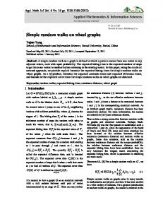
Let A be a countable alphabet. Two words w and w0 are conjugate, denoted by w ∼ w0 , iff w = uv and w0 = vu for some u, v in A∗ (the set of finite words over A). They are equivalent, denoted by w ≡ w0 , iff w ∼ w0 or w e ∼ w0 (where w e is the mirror image of w). We let D(A) be the set of words over A having two occurrences or no occurrence of each letter. The elements of W (A), defined as the quotient set D(A)/ ≡, are called double occurrence words. They will be used to represent the crossing points of closed curves. The word abcabc represents the curve on the left of Figure 1. In order to associate combinatorial objects with sets of intersecting closed curves, we define the notion of a double occurrence multiword : this is a multiset of ≡-equivalence classes of words, m = {[w1 ]≡ , ..., [wn ]≡ } such that w1 w2 ...wn ∈ D(A). We denote by M W (A) the set of double occurrence multiwords on A. In writing them, we will omit the brackets [...]≡ and when defining m = {w1 , ..., wn }, the order of the words w1 , ..., wn is irrelevant. We denote by V (m) the set of letters which occur in m. The two curves on the right of Figure 1 yield the double occurrence multiword {abdecabc, df f e}. Let C be a closed curve in the plane, with finitely many self-intersections but no triple self-intersection. We name each crossing point by a letter from A. By following the curve from some point and by retaining the names of the crossing points, we obtain a double occurrence word over A. Changing the starting point and/or the direction of traversal yields an ≡-equivalent word on A∗ , hence the same double occurrence word. We denote by w(C) the common equivalence class of the words associated with C. Such words are called Gauss words. If C has no self-intersection, i.e. if it is homeomorphic to a circle, w(C) is the empty word. Some double occurrence words like abab are not Gauss words as one checks easily. Gauss words are characterized in several articles by Lovasz and Marx [LM], Rosenstiehl [Ros], and de Fraysseix and Ossona de Mendez [FOM] to name a few. These works are reviewed in the book by Godsil and Royle [GodRoy]. Two non-homeomorphic such curves may define a same word. An example is the word abba. Two curves defining it are shown on Figure 3. We will characterize the Gauss words which characterize a unique curve, where as usual, unicity is understood up to homeomorphism (Theorem 3.4 below). 5

Figure 2: Intersecting closed curves

Figure 3: Two 4-regular plane graphs with same weak map With a set of closed curves C1 , ..., Cn in the plane with no triple point, we associate the double occurrence multiword Γ(C1 , ..., Cn ) = {w(C1 ), ..., w(Cn )}. We call Γ(C1 , ..., Cn ) a Gauss multiword. It is clear that changing the starting point and/or the direction of traversal of one or several curves yields the same double occurrence multiword. Examples are {ε, ε, ε}, {abcabdec, df f e} and {abcd, abcd}. The first one corresponds to three disjoint circles, the second one is defined by two curves shown on Figures 1 (right part) and the third one by two curves shown on Figure 2. This example shows that multisets are actually necessary. The plane can be replaced by a 2-dimensional compact surface Σ. This yields the notions of a Σ-Gauss word and of a Σ−Gauss multiword. The word abab is associated with a curve on the torus shown on Figure 4. We say that a set of curves on a surface is connected if it defines a connected subset of the surface. It is connected iff the corresponding multiword is not the union of two multiwords on disjoint subsets of A.

2.2

Graphs, maps and walks

We will consider (finite) graphs without isolated vertices, and possibly with loops and multiple edges. For a graph G with set of vertices VG , set of edges EG , we will write e : x − y to express that the undirected edge e links x and y. Occasionally, we will consider directed graphs. We will use the notation e : x −→ y to express that e is a directed edge from x to y. A graph is 4-regular iff every vertex has degree 4. A loop counts for 2 in the degree of its vertex.

6

Figure 4: A curve on the torus

Maps are combinatorial objects that formalize embeddings of graphs in oriented surfaces. Let E be an embedding of a graph G in an oriented surface. (See the books by Mohar and Thomassen [MT] or Ringel [Rin] for precise definitions). Around a vertex, the incident edges form a circular order if they are looked at in turn according to the orientation of the surface. Because these edges may be loops, we will have to use half-edges in order to distinguish the two incidences of a loop with a vertex. For every edge e of an embedded graph G, we choose arbitrarily an orientation (unless one is already given) and we define two half-edges e1 , e2 called darts. If e : x −→ y we let e1 be incident to x and the other to y. If x 6= y, we denote e1 by (x, e) and e2 by (y, e). We denote by DG the set of darts of G. We let α be the permutation of DG such that e1 = α(e2 ) and e2 = α(e1 ) for e ∈ EG . Its orbits correspond to the edges. We let σ be the permutation of DG such that fj = σ(ei ) where ei and fj represent incidences of edges e and f with a same vertex x and fj follows ei in the circular ordering of incidences around x, relative to E. We call M (E) =< DG , α, σ > the map describing the embedding E of G. More generally, a map is a triple M =< DM , αM , σM > such that DM is a set of even cardinality called the set of darts, αM and σM are permutations of DM and αM is involutive without fixed points. It is 4-regular iff each orbit of σM has 4 elements. An example of a 4-regular map is shown in Figure 5. The vertices are a, b, c and the darts are numbered from 1 to 12. Let M = M (E). If we change the orientation of the surface (or in the case of the plane, if we replace E by its image under the symmetry relative to a straight line) then the map of the corresponding embedding is obtained by replacing σM −1 by σM . We denote it by M −1 and call it the symmetric map of M . To every map M =< D, α, σ > corresponds a graph G = Graph(M ) defined as follows : VG is the set of orbits of σ, EG is the set of orbits of α, and [d]α : [d]σ − [α(d)]σ for all d in D, where [d]α denotes the orbit of d under α and similarly for [d]σ . We say that [d]σ (resp. [d]α ) is the vertex (resp. the edge) defined by d. It is 4-regular iff its graph is 4-regular. A walk in a map M =< D, α, σ > is a sequence of darts w = (d1 , ..., d2n ) such that, for each relevant i, d2i = α(d2i−1 ) and d2i+1 and d2i define the

7

Figure 5: A 4-regular planar map

same vertex. The walk is closed if d1 and d2n define the same vertex. There corresponds to w a walk in Graph(M ) defined as : (v1 , e1 , v2 , ..., en , vn+1 ) where vi is the vertex defined d2i−1 (and vn+1 = v1 is defined by d2n ), and ei is the edge defined by d2i for each i. The opposite walk (vn+1 , en , vn , ..., v2 , e1 , v1 ) is defined from the opposite walk in the map : (d2n , ..., d1 ). Maps on surfaces

A map M is planar if it is associated with an embedding of Graph(M ) in the plane (or in the sphere). It is a Σ−map if it is associated with an embedding of Graph(M ) in an oriented surface Σ. An embedding of a graph on a surface is proper if the complement of the graph (a finite union of curve segments, hence a closed set) is a union of open sets, each homeomorphic to an open disk. If two proper embeddings of a graph yield two equivalent maps, i.e., maps that are equal or symmetric, then they are homeomorphic. (Theorem 3.2.4 of [MT] ; this applies to the sphere, not to the plane). We will consider them as the same embedding. Hence, two equivalent maps specify a "unique" proper embedding on a unique surface Σ. A map M =< D, α, σ > is planar iff it satisfies Euler’s equality z(σ) − z(α) + z(σ ◦ α) = 2, where z(π) denotes the number of orbits of a permutation π. For an oriented surface of genus g, the characteristic equality is z(σ) − z(α) + z(σ ◦ α) = 2 − 2g. A pointed map is a pair (M, d) where d is a dart. If M is connected and planar, there is a unique planar embedding (up to a homeomorphism of the plane) such that the closed walk (d1 , ..., d2n ) with d1 = σ(d), d2 = α(σ(d)), d2i+1 = σ(d2i ) for each i > 0 is the border of the unique infinite topological face, which lies to the right of the walk. The embedding of the map M shown in Figure 5 is defined by the pointed maps (M, 4), (M, 8) and (M, 12). More definitions : Submaps, G-maps, Ae -maps, Av -maps. Let M =< D, α, σ > be a map. A map N =< DN , αN , σN > is a submap of M if DN ⊆ D, αN is the restriction of α to DN and σN (d) = σ n (d) where n is the least positive integer such that σ n (d) ∈ DN . If X is a subset of D and 8

DN = X ∪ α(X), we say that N is the submap of M induced by X. If M is the map of an embedding of a graph G in a surface, then N is the map of the induced embedding of the subgraph of G consisting of all edges defined by the darts in X. An isomorphism of maps M =< D, α, σ > −→ M 0 =< D0 , α0 , σ 0 > is a bijection h : D −→ D0 such that α0 ◦ h = h ◦ α, σ 0 ◦ h = h ◦ σ. It yields an isomorphism h : Graph(M ) −→ Graph(M 0 ). Intuitively, M and M 0 define the same embedding in some surface of the graph Graph(M ). We make this more precise. Let G be a graph. A G-map is a pair (M, g) where g is a graph isomorphism Graph(M ) −→ G. An isomorphism of G-maps (M, g) −→ (M 0 , g 0 ) is an isomorphism h : M −→ M 0 such that g 0 ◦ h = g. Let A be a countable alphabet. An Ae -map (shorthand for map with edges named in A) is a pair (M, g) where M is a map and g is one-to-one : EM −→ A. (We let EM denote EGraph(M) and VM denote VGraph(M) ). The mapping g gives names to the edges of Graph(M ). An isomorphism of Ae -maps h : (M, g) −→ (M 0 , g 0 ) is an isomorphism of maps that preserve the names of edges, i.e., such that g 0 ◦ h = g. Similarily, an Av -map (shorthand for map with vertices named in A) is a pair (M, g) where M is a map and g is one-to-one : VM −→ A. The mapping g gives names to the vertices of Graph(M ). An isomorphism of Av -maps is an isomorphism of maps that preserves the names of vertices. Isomorphism is denoted by '. We will use the notations 'G , 'e and 'v to stress that we consider isomorphisms of G-maps, of Ae -maps or of Av -maps. Remark : There exists another more complicated way to specify maps, which works also for nonoriented surfaces. Each edge is split into 4 flags, instead of 2 darts. These objects formalize the left and right sides of each edge. See Crapo and Rosensthiel [CraRos], Lins et al. [Lins, LRS] or the book by Godsil and Royle [GodRoy].

2.3

Weak maps and straight walks

The weak map associated with a 4-regular map M =< D, α, σ > is the structure W eak(M ) =< D, α, σ 2 , neigh > such that neigh is the binary relation {(d, σ(d)), (σ(d), d) | d ∈ D}. We say that two darts a, b such that neigh(a, b) holds are neighbour. It is clear that W eak(M ) = W eak(M −1 ) because σ 2 = (σ−1 )2 and neigh is invariant under taking the inverse of σ. Figure 3 shows two different maps with same weak maps (their vertices are a and b). More generally, a weak map is a structure W =< D, α, ω, neigh > where D is the set of darts, α and ω are involutive permutations without fixed points, neigh is a symmetric binary relation defining a union of pairwise disjoint 4-cycles and ω exchanges opposite elements on these cycles. We say that two darts d, d0 such that d = ω(d0 ) are opposite. A 4-regular graph Graph(W ) is associated with it in an obvious way. An embedding of W in a surface is an embedding E of Graph(W ) such that W = W eak(M (E)).

9

The notions of weak G-map, weak Ae -map and weak Av -map extend immediately from the case of maps. Isomorphism is denoted by ', 'G , 'e and 'v in the obvious way. Let M =< D, α, σ > be a 4-regular map. A straight walk in M is a walk (d1 , d2 , ..., dk ) such that d2i+1 = σ(σ(d2i )) for all i > 0. The notion of a straight walk depends only on α and σ 2 . From each dart d1 , we get a unique straight closed walk (d1 , d2 , ..., d4n ) such that d1 = σ(σ(d4n )). The graph Graph(M ) is thus a union of edge-disjoint closed walks where each vertex occurs once in two of them or twice in a single one. (In other words, we have a cover by edge-disjoint cycles, hence we have an Eulerian tour in the case of a unique cycle.) For an Av -map (M, g) we denote by Γ(M ) (we omit the reference to g) the corresponding double occurrence multiword on A, where each vertex x is replaced by g(x). The notion of a straight walk of a 4-regular map depends only on the associated weak map. We can thus define Γ(W ) for a weak map W in such a way we have Γ(M ) = Γ(W eak(M )). Lemma 2.1 : A weak Av -map W is defined, up to isomorphism of Av -maps by Γ(W ) ∈ M W (A). Proof : A double occurrence multiword m in M W (A) can be given as a 4-tuple P (m) =< P, suc, slet, (leta )a∈A > where P is the set of occurrences of letters in m, suc is the successor relation on P (the elements of m are circular words up to reversal but for each of them we choose a traversal direction), slet is the symmetric binary relation expressing that two occurrences have the same letter, and leta (x) holds iff a is the letter at position x. Then, we associate with m the weak map W =< D, α, ω, neigh > with set of vertices V (m) (the set of letters occuring in m) defined as follows. The permutation ω is actually handled as a symmetric binary relation. D = P × {out, in}, α(x, out) = (y, in) and α(y, in) = (x, out) if suc(x, y) holds, ω((x, out), (x, in)) and ω((x, in), (x, out)) hold for all x in P , neigh(u, v) holds if u ∈ {x} × {out, in}, and v ∈ {x} × {out, in} for some x ∈ P , where for each x, we let x denote the unique element such that slet(x, x). The vertex incident with the darts in {x, x}×{out, in} is named a if leta (x). We denote by W (m) the weak Av -map associated in this way with m ∈ M W (A). Claim : Γ(W (m)) = m and W (Γ(M )) 'v M for every weak map M . The verification is routine. This claim yields the result.¤ Remark : In the sequel, we will omit the sets leta in the relational structures representing double occurrence multiwords because the identity of letters does not matter. What matters is only the fact that two positions have the same

10

letter. For an example the Gauss multiword of the two curves on the right of Figure 1 is represented by the relational structure : P ({abcabdec, df f e}) =< {1, ..., 12}, suc, slet > with suc = {(1, 2), (2, 3), ..., (8, 1), (9, 10), (10, 11), (11, 12), (12, 9)}, slet = {{1, 4}, {2, 5}, {3, 8}, {6, 9}, {7, 12}, {10, 11}}. Curves, 4-regular maps and Gauss multiword.

Convention : From now on, "surface" means "orientable surface" like the plane (or the sphere) or the sphere with handles. Let S = {C1 , ..., Cn } be a set of closed curves in the plane or in an orientable surface Σ, with no triple point. It defines a 4-regular graph G(S) embedded in the considered surface : the vertices are the intersection points, and the curve segments between the intersection points represent the edges. Moreover, it defines a 4-regular map M (S). For this map, two consecutive segments on a curve with common end point v (a vertex of G(S)) define two opposite darts. Hence each curve is the union of the segments corresponding to edges of the closed straight walks in M (S). Let conversely M be a 4-regular map embedded in a surface Σ. Its closed straight walks form a set SM of intersecting curves and M (SM ) = M . It is clear that Γ(SM ) = Γ(M ). Hence, sets S of intersecting curves will be handled as 4-regular maps. This gives a combinatorial formalization suitable for expressing their properties in Monadic Second-order logic. Actually, we will mainly consider connected sets of curves (excluding the case of a single curve with no self-intersection) represented by connected 4-regular maps. Consider two sets S and S 0 of intersecting curves on a surface, with same Gauss multiword Γ(S) = Γ(S 0 ), that are not necessarly homeomorphic. The corresponding graphs are the same but the maps M (S) and M (S 0 ) may be different (i.e., not Av -isomorphic, even up to symmetry). However, W eak(M (S)) 'v W eak(M (S 0 )) by Lemma 2.1. Hence, Γ(S) = Γ(S 0 ) iff W eak(M (S)) 'v W eak(M (S 0 )). To summarize, sets of curves are handled as 4-regular maps and the associated double occurrence multiwords are in bijection with weak maps. Here is the picture : sets of curves up to homeomorphism on Σ ←→ 4-regular maps ↓ ↓ Σ-Gauss multiwords ←→ straight walks ←→ weak maps

11

2.4

Constructions and characterizations in Monadic Secondorder logic

Monadic Second-order (MS in short) logic is reviewed in Appendix. As in the reference articles, definitions are given for relational structures. However a map defined as a triple < D, α, σ > is not, strictly speaking, a relational structure because α and σ are mappings D −→ D and are not binary relations. However, we will consider these mappings as binary relations in the usual way, and without introducing a specific transformation of functions into relations, we will consider maps and weak maps as relational structures. We will frequently use the following fact stated formally as backwards translation in Proposition A.1 of Appendix : if τ is a mapping from graphs to graphs (or more generally from relational structutres to relational structures) defined by MS formulas, we will call τ an MS transduction, then every MS property of T = τ (S) can be expressed as an MS property of the relational structure S. Proposition 2.2 : Let Σ be a surface. That a map or a weak map is embeddable in Σ is MS definable. Proof: For maps, this is proved in [CouDus] with the help of a characterization of Σ−maps in terms of finitely many excluded minor-maps. (The characterization by Euler equality cannot be used because one cannot count in MS logic.) We now consider the case of a weak map W =< D, α, ω, neigh >. Our objective is to specify a map M such that W eak(M ) = W , in terms of two subsets X and Y of D. If M is a 4-regular map < D, α, σ > such that W eak(M ) = W , if d and e are two darts such that e = σ(d), then the restriction of σ to the σ-orbit of d can be determined from d, e, ω by the following first-order formula : y = σ(x) :⇐⇒ (x = d ∧ y = e) ∨ (x = e ∧ ω(y, d)) ∨ (ω(y, e) ∧ ω(x, d)) ∨ (y = d ∧ ω(x, e)). Hence the permutation σ on D can be specified by two disjoint subsets X and Y of D such that : (*) Every vertex v is defined by one and only one dart d in X and also by one and only one dart e in Y , and furthermore neigh(d, e) holds. Assuming satisfied this condition on X, Y, there is unique map M (W, X, Y ) =< D, α, σ > such that W eak(M (W, X, Y )) = W and σ(d) ∈ Y for every d ∈ X. Hence, W is a Σ−weak map iff there exist disjoint sets X and Y satisfying (*) such that M (W, X, Y ) is a Σ−map. By the first assertion and the method of backwards translation (cf. Proposition A.1), we obtain that this property is expressible by an MS formula. Let us detail the argument. The mapping associating the relational structure M (W, X, Y ) with the structure 12

W 0 consisting of W enriched with the two sets X and Y is an MS transduction τ . That the output M (W, X, Y ) is a Σ−map can be expressed by an MS formula. This formula can be translated backwards (wrt τ ) into an equivalent MS formula to be evaluated in W 0 . This formula has the form ϕ(X, Y ) since it depends on X and Y . The desired MS formula is thus ∃X, Y.ϕ(X, Y ) . ¤ The following Proposition contains a logical version of Lemma 2.1. Proposition 2.3 : The mapping Γ from weak maps to multiwords and its inverse are MS transductions. Proof : We first prove that Γ is an MS transduction. Let W =< D, α, ω, neigh > be a weak map. Claim : There exists a subset X of D satisfying the following conditions : 1) every vertex of Graph(W ) is defined by exactly two darts in X, which furthermore are neighbours (this is specified by neigh), 2) for every d ∈ X there exists e ∈ X such that ω(α(d), e) holds. Proof of claim : For each closed straight walk of W , we choose a representing sequence of darts w = (d1 , ..., d2n ), and we let X be the set of darts with odd indices of all these sequences. It satisfies Condition 1) because at every vertex, either two closed straight walks cross, or one crosses itself, and Condition 2) by the definition of straight walks. Conversely, every set X satisfying Conditions 1) and 2) is associated as above with choices of directions of traversal for the closed straight walks of W . From W and such a set X we define a relational structure P =< X, suc, slet > by : suc = {(d, d0 ) | d, d0 ∈ X, ω(α(d), d0 )} slet = neigh ∩ (X × X). It is then clear that P is isomorphic to P (Γ(W )), the relational structure describing Γ(W ) (cf. Lemma 2.1). The identity of letters is omitted. This shows that Γ is an MS transduction with one parameter X. Actually, for all choices of the set X satisfying 1) and 2), the associated structures are isomorphic. That Γ−1 is an MS transduction is actually proved by the construction of Lemma 2.1. ¤ Corollary 2.4 : For every surface Σ, the property of a multiword that it is a Σ−Gauss multiword is expressible by an MS formula. Proof : Let a multiword m be given by the relational structure P (m). The corresponding weak map Γ−1 (P (m)) is definable from P (m) by an MS transduction by Proposition 2.3. By Proposition 2.2, an MS formula can express that the weak map Γ−1 (P (m)) is embeddable in Σ. It follows by backwards

13

translation (see Proposition A.1 of Appendix) that this can be expressed in P (m) by an MS formula. This completes the proof. However, for the particular case of the plane and of a singleton m = {w}, another proof can be given. For a in V (w), we let N (a) be the set of letters b such that w ≡ aubvau0 bv 0 for some words u, v, u0 , v 0 . Rosensthiel proves in [Ros] (another proof is given in [FOM]) that w is a Gauss word iff there exists a bipartition (E, F ) of V (w) such that for every a, b ∈ V (w), a 6= b the cardinality of γ(a) ∩ ω(b) is even, where γ(a) = N (a) ∪ {a} and ω(a) = N (a) if a ∈ E, γ(a) = N (a) and ω(a) = N (a) ∪ {a} if a ∈ F . This is expressible by a C2 MS formula in the structure P ({w}), where C2 means that we may use the set predicate Even expressing even cardinality. This is MS expressible in the structure P ({w}) because a linear order on this structure is MS definable (routine argument, [CouX]), and thus the predicate Even(X) is itself MS definable. ¤ Remark : The first construction in this proof is not only more general than the second one but it is also more informative because, by the results of [CouDus], we can not only express in MS logic that a map is embeddable in a surface Σ but we can also specify an embedding when one does exist. Here, we can express in MS logic that a given multiword is a Σ−Gauss multiword, and we can also specify, in terms of 4-regular maps and by MS formulas, an embedding of the corresponding graph in Σ, hence actually a set of curves. Corollary 2.5 : The mapping that associates with a double occurrence multiword m the set of sets of curves on a fixed surface Σ having m as associated multiword is an MS transduction. Proof : Immediate consequence of Propositions 2.3 and 2.2. ¤ Although we have a logical characterization, we are not fully satisfied because it gives nothing about the common structure of the sets of curves having a same associated Σ−Gauss multiword. We will obtain in Section 6 a structural description for the case of the plane.

3

Weak maps having a unique planar embedding and unambigous Gauss words

The main theorem of this section characterizes as the prime multiwords those which describe a unique set of curves on the plane, where unique is understood as usual, up to an homeomorphism of the sphere. Using Whitney’s Theorem saying that a simple and 3-connected graph has a unique planar embedding (see any textbook in graph theory, e.g., [Die], or the book on graph and surfaces [MT]), we give a similar condition for planar weak maps. This is the main lemma for 14

the proof of the theorem. The condition of 2-connectivity is necessary as shows Figure 3, but it is is not strong enough to yield unambiguity of the associated Gauss multiwords. Proposition 3.1 : A planar weak map without loop, such that any two distinct vertices are linked by 3 edge-disjoint paths has a unique planar embedding. We need some definitions and lemmas. Let M be a 4-regular map or a weak map and let w = (d1 , ..., d2n ) and z = (f1 , ..., f2m ) be two walks in M . We say that they cross at a vertex x of Graph(M ) if for some even i and j with 1 < i < 2n, 1 < j < 2m we have x = {di , di+1 , fj , fj+1 }, di and di+1 are opposite, and so are fj and fj+1 . Two walks are noncrossing if they cross at no vertex. Lemma 3.2 : If in a weak map there are k edge-disjoint path from u to v 6= u (necessarily, k ≤ 4), then there are k pairwise noncrossing edge-disjoint paths from u to v. Proof : Each set of k edge-disjoint path from u to v, can be replaced by a set of k edge-disjoint paths from u to v, with one less crossing point. Because if two edge disjoint paths e1 − e2 − ... − en and f1 − f2 − ... − fp from u to v cross at x incident with ei , ei+1 , fj and fj+1 we can replace them by the paths e1 −e2 −...−ei −fj+1 −fj+2 −...−fp and f1 −f2 −...−fj −ei+1 −ei+2 −...−en . We still have exist k pairwise edge-disjoint paths from u to v with one less crossing. We can repeat this step until we have no crossing at all.¤

Definition : Graphs encoding weak maps With a weak map W =< D, α, ω, neigh >, we associate a graph H(W ), the planar embeddings of which determine all those of W . Here is the construction. We let G = Graph(W ). We let H(W ) be the undirected graph with set of vertices VG ∪ D, and edges of three types : the edges defined by α (between two elements of D), the edges d − v, where d ∈ D and v ∈ VG is the vertex defined by d, and finally the edges d − d0 for d, d0 ∈ D such that neigh(d, d0 ) holds. Intuitively, on an edge e of G, we put two new vertices, defined concretely as the two darts forming this edge. We define edges between these new vertices that "materialize" the neighbourhood relation neigh.

This is illustrated in Figure 6 : since neigh((u, e), (u, h)) holds, such a new edge is created between the new vertices x and t. In any planar embedding of H(W ), the (subdivided) edges e, h, f, g must be placed according to the constraints of W , in particular, e and f must be "opposite". 15

Figure 6: From W to H(W )

Lemma 3.3 : If W is a weak map without loop, such that any two distinct vertices are linked by 3 edge-disjoint paths, the graph H(W ) is simple and 3-connected. Proof : Let G = Graph(W ). The only possibility that H(W ) is not simple is in the case where α(d) = σ(d) for some d, which cannot happen if W has no loop. For proving 3-connectedness, we consider two vertices a and b of H(W ), and we want to prove that there are 3 vertex-disjoint paths in H(W ) linking them. Case 1 : a and b are both vertices of G . By Lemma 3.2, there are 3 edge-disjoint noncrossing paths between them. They yield 3 vertex disjoint paths in H(W ) because, since the considered paths in G are not crossing, if two paths share a vertex u (see Figure 6) with e, g on one path, both incident to u, and f, h on the other, then, in H(W ) we can avoid u and use instead x − y on the first path and t − z on the other. Case 2 : None of a and b is a vertex of G. There are vertices a and b in G respectively neighbours of a and b. Subcase 1 : a = b We need only look at Figure 6 considering that a = b = u and a and b are both in {x, y, z, t}. There are 3 vertex disjoint paths between a and b. For example if x = a and y = b, the three paths are x − y, x − u − y, x − t − z − y. The other cases are similar. Subcase 2 : a 6= b Again Figure 6 will help. Let u = a. As in Case 1, there are 3 edge-disjoint noncrossing paths between a and b. These paths, say pe , pf , pg , start from u = a and use respectively the edges e, f, g. They can be made to start from x = a : the path pf is modified to start with x − u − z, the path pg to start with x − y, and the path pe to start at x, avoiding u, t, y. By applying this observation also to b and b instead of a and a respectively, we obtain 3 vertex-disjoint paths, as in the first case. 16

Case 3 a is in G and b is not. Subcase 1 : b is neighbour of a. Using Figure 6, we have a = u and, say, b = x. The three paths are u − x, u − t − x, u − y − x. Subcase 2 : b is neighbour of b in G, b 6= a. The proof is as in the second subcase of Case 2. ¤ Proof of Proposition 3.1 : Let W be planar weak map without loop, such that any two distinct vertices are linked by 3 edge-disjoint paths. It has a planar embedding E. By adding on each edge two vertices corresponding to the two darts and edges according to the definition of the transformation H, one obtains a planar embedding E H of H = H(W ). See Figure 6. This embedding is described by a map NE such that Graph(NE ) = H. The map M (E) is defined from NE by deletions and contractions of edges. (See Courcelle and Dussaux [CouDus] for deletions and contractions of edges in maps ; in a few words, they preserve embeddings). Assume now that F is another planar embedding of W . From it we define similarly NF . Hence Graph(NE ) = Graph(NF ) = H. Since H is simple (because W has no loop) and 3-connected (by Lemma 3.3), it has a unique planar map, hence NE = NF or NE = NF−1 . Since M (E) and M (F) are defined from NE and NF by the same edge deletions and contractions, we have M (E) = M (F) or M (E) = M (F)−1 as was to be proved.¤ Remark : If W is a planar weak map and G = Graph(W ) is separable, then some planar embeddings of H(W ) may correspond to no planar embedding of G. Definition : Unambigous and prime Gauss multiwords A Gauss word or multiword m is unambigous if the corresponding weak map W (m) has a unique planar embedding. A double occurrence word is prime if it is not ε and is not (≡ −equivalent to) a concatenation of nonempty double occurrence words. Hence, aa and abab are prime whereas abba is not. A double occurrence multiword is prime if it is connected, not empty, is not {ε} and is not a product of two double occurrence multiwords, where we say that {u1 w1 , u2 , ..., un , w2 , ..., wp } is a product of {u1 , u2 , ..., un } and {w1 , w2 , ..., wp }. Note that two multiwords have several products. For examples {abcd, abcd} is prime whereas {abcd, ab, cd} is not. The prime multiword {abcd, abef, cdf e} corresponds to the curves of Figure 7. Theorem 3.4 : A connected Gauss multiword with at least 2 letters is unambigous iff it is prime. Proof : "Only if" direction. Let m be a connected Gauss multiword with at least 2 letters that is not prime. Hence m = {u1 w1 , u2 , ..., un , w2 , ..., wp } is 17

Figure 7: Three overlapping circles

a product of m1 = {u1 , u2 , ..., un } and m2 = {w1 , w2 , ..., wp } where the subsets V (m1 ) and V (m2 ) of A are disjoint. Let M =< D, α, σ > be a planar map such that W eak(M ) = W (m). Let G = Graph(W (m)). Its set of vertices is V (m1 ) ∪ V (m2 ). Let Di be the set of darts of M that define a vertex in V (mi ). We define the map M 0 =< D, α, σ 0 > by letting σ 0 (d) = σ(d) if d ∈ D1 and 0 σ (d) = σ −1 (d) if d ∈ D2 . It is clear that W eak(M 0 ) = W eak(M ). We claim that M 0 is planar. Consider an embedding of M . The vertices of V (m2 ) and the edges between them form a connected part, linked to the remaining by two edges. This part can be flipped, (this corresponds to replacing σ by σ −1 on D2 , hence to replace the portion of the drawing induced by V (m2 ) by a symmetric one) while preserving the linking edges. (An example can be seen on Figure 3 : the map to the right is obtained from that to the left by flipping the part corresponding to b. In this example, D2 is the set darts incident with vertex b.) This gives a planar embedding of M 0 . It is clear that M 0 is neither G−isomorphic to M nor to M −1 . Hence the multiword m is ambigous. ¤ One more lemma is needed for the other direction. Lemma 3.5 : If m is a prime Gauss multiword with at least 2 letters, the multigraph Graph(W (m)) is 4-edge-connected. That Graph(W (m)) is 3-edge-connected suffices actually for the sequel. Proof : We first assume that m consists of a single word w of length at least 4. The graph G = Graph(W (m)) has set of vertices V (w) and an undirected edge a − b (possibly a loop) for each occurrence of a followed by an occurrence of b. Let G0 be G minus 3 edges. We claim that G0 is connected. Choosing 3 edges in G amount to writing w ∼ w1 w2 w3 , where w1 , w2 , w3 are nonempty and the chosen edges are between the last position in w1 (resp. w2 , w3 ), and the first position in w2 , (resp. w3 , w1 ). Let Ai = V (wi ). Each induced subgraph G0 [Ai ] is connected (because the positions in wi define a traversal of this graph). If A1 has no letter in common with A2 and A3 , then w1 is a double occurrence word and w is not prime. Hence wlog, we have a letter a in A1 ∩ A2 . 18

Similarly, we have b in A2 ∩ A3 . It follows that any two letters in V (w) are connected by a path in G0 built from paths in the graphs G0 [Ai ]. Hence G0 is connected, and G is 4-edge connected. We now extend this proof to the case of a multiword m. We define G and G0 in the same way. We distinguish three cases to adapt the above proof. Case 1 : the 3 deleted edges are from a same word in m. We have m = {w1 w2 w3 , w4 , w5 , ..., wn }. Then we let Bi = V (wi ) . We defineSa binary relation R by letting iRj iff Bi ∩ Bj 6= ∅. For i = 1, 2, 3 we let Ai = {Bj | iR∗ j} and C = V (m) − A1 ∪ A2 ∪ A3 . If C is not empty, then m is not prime because it can be expressed as m = {w1 w2 w3 , ...}∪m0 where m0 is the multiset of words wj , for j with Bj ⊆ C. Hence V (m) = A1 ∪ A2 ∪ A3 . Each induced subgraph G0 [Ai ] is connected. If A1 has no letter in common with A2 and A3 , then w is not prime because it can be written as a product of {w1 , ...} and {w2 w3 , ...}. For the same reason, at least one of A2 ∩ A3 and A1 ∩ A3 is not empty. It follows that G0 is connected. Case 2 : 2 deleted edges are in a same a same word in m. Hence, we have m = {w1 w2 , w3 , u1 , u2 , ..., un } and the deleted edges are between the last position in w1 (resp. w2 , w3 ), and the first position in w2 , (resp. w1 , w3 ). The argument is essentially the same as in Case 1. Case 3 : The three deleted edges are in different words in m. Hence, we have m = {w1 , w2 , w3 , u1 , u2 , ..., un } and the deleted edges are between the last position in w1 (resp. w2 , w3 ), and the first position in w1 , (resp. w2 , w3 ). The argument is essentially the same as in the previous two cases. Hence, we obtain that G is 4-edge-connected.¤ Proof of Theorem 3.4. End : Let m be a prime Gauss multiword with at least 2 letters. The weak map W (m) has no loop (otherwise m can be factorized as {aa}m0 ), it is 4-edge-connected by Lemma 3.5, hence 3-edge-connected and, by Proposition 3.1, it has a unique planar embedding and m is unambigous.¤ Remarks : 1) The "if" direction of Theorem 3.4 is proved with a different technique and for the particular case of Gauss words (and not of multiwords) by Chaves and Weber in [ChaWeb]. 2) Whether a multiword is prime is easily expressible by an MS formula. It follows that the characterization of unambigous Gauss multiwords of Theorem 3.4 is expressible by an MS formula. The notion of unambiguity can be defined for Σ-Gauss multiwords, but we have no characterization similar to Theorem 3.4. However, one can express this property in MS logic. The construction is based on the proof of Proposition 2.2. We let W be a weak map and (X, Y ) and (X 0 , Y 0 ) be two pairs of sets of darts satisfying condition (*) of the proof of this proposition. It is straightforward the express by an MS formula the property : (**) M (W, X, Y ) = M (W, X 0 , Y 0 ) or M (W, X, Y ) = M (W, X 0 , Y 0 )−1 .

19

Hence, W is uniquely embeddable in a surface Σ iff it is embeddable in Σ and, for every 4-tuple of sets of darts (X, Y, X 0 , Y 0 ), if (X, Y ) and (X 0 , Y 0 ) satisfy condition (*) then they satisfy condition (**). This is expressible in MS logic. It remains an open question to understand combinatorially the unique embeddability property of Gauss multiwords in surfaces. (The article by Negami [Neg] which characterizes the maps which are uniquely embeddable in the torus might help). The picture is here : certain sets of curves up to homeo ←→ 4-regular 3-edge-connected maps l l prime Gauss m-words ←→ straight walks ←→ 3-edge-connected weak maps

In order to understand the case of Gauss multiwords that are not prime, and to understand the structure of the set of all sets of curves defining one of them, we introduce new notions.

4

Diagonal walks and medial maps

In this section, we recall that sets of curves on the plane are in bijection with the so-called diagonal walks on planar maps. These walks are actually the straight walks of a 4-regular map called the medial map of the considered map. Since every 4-regular planar map is the medial map of some map, we obtain in this way another characterization of Gauss multiwords. The main references for this section are Richter [Ric], Archedeacon et al. [ABL], Crapo and Rosenstiehl [CraRos] or the book by Godsil and Royle [GodRoy]. We recall that the medial maps of a map and of its dual are the same. Most of the results of this section hold for all maps, not only for planar ones. Some proofs in the planar case are easier because they can be based on plane embeddings and take advantage of geometric intuition.

Diagonal walks A diagonal walk in a map M =< D, α, σ > is a closed walk (d1 , d2 , ..., d4n ) such that d2i+1 = σ(d2i ), if i is odd and 1 ≤ i ≤ 2n − 1, and d2i+1 = σ −1 (d2i )) if i is even and 2 ≤ i ≤ 2n (with d4n+1 = d1 ). The corresponding walk in Graph(M ) is also called a diagonal walk (this notion depends on the considered map). We identify in both cases a diagonal walk and its opposite walk (which is also diagonal), and we also consider (d1 , d2 , ..., d4n ) and (di+1 , ..., d4n , d1 , ..., di ) as the same walk. 20

Figure 8: A map M0

It is a classical fact that D is the union of the sets {d1 , d2 , ..., d4n } arising from all diagonal walks. Each dart occurs twice in a same set or once in two sets. These sets yield a set of closed walks of the graph where each edge has two occurrences, either in a same walk or in different ones. For an Ae -map N = (M, g), we denote by ∆(N ) ∈ M W (A) the double occurrence multiword which is the image under g of the circular sequences of edges of the diagonal walks, and we call it the diagonal of N. (We recall that the components of multiwords are defined up to reversal and conjugacy, and so are closed walks.) Clearly we have ∆(M −1 ) = ∆(M ) because if (d1 , d2 , ..., d4n ) is a diagonal walk for M , then (d3 , ..., d4n , d1 , d2 ) is one for M −1 , and is defined as "the same". In the example of Figure 5, let us name u, v, w, x, y, z the edges (4,5), (3,6), (1,12), (2,11), (7,10), (8,9) respectively. Then ∆(M ) = {wzyx, yzuv, wxvu}. A map is diagonally connected if ∆(M ) is singleton. Such maps are characterized algebraically in [Ric, ABL, CraRos, GodRoy] as those such that Graph(M ) has no set of edges which is both a cycle and a cocycle. For the map M0 of Figure 8, ∆(M0 ) = {eabdcbacdef hgf mmhg}. It is diagonally connected. The corresponding walk is shown in Figure 10 (where the edges of the map M0 are traversed rather than followed). Medial maps Let M =< D, α, σ > be a map with G = Graph(M ). In order to help the understanding of the definition, we first describe H = Graph(M edial(M )). Its set of vertices is EG (the set of edges of G). Its set of edges is D. The two end vertices of an edge d are [d]α and [σ(d)]α . Intuitively, the middle points of edges of G are made into vertices of H, and these vertices are linked by an edge in H if they correspond to consecutive edges around a vertex of G (consecutive with respect to the map M ). We now define M edial(M ). Its set of darts is D × {+, −}, the two darts of an edge d are (d, +) and (σ(d), −), and the "next dart" permutation σMedial(M) 21

Figure 9: The map M edial(M0 ) : detail

associates (d, −) with (d, +) and (α(d), +) with (d, −) for all d in D. From this construction it is clear that the mapping from M to M edial(M ) is an MS transduction. If M is embeddable in a surface, then M edial(M ) is embeddable in the same surface. This is clear from the construction with help of Figure 9. Using an embedding of M , one can place a vertex e of M edial(M ) (which is an edge of M ) in the middle of the segment representing this edge, and draw an edge of M edial(M ) with two darts (d, +) and (σ(d), −) by a segment in the face defined by d and σ(d), "close" to the half-edges of M associated with these darts. For an example, consider the map M0 of Figure 8. We have EG = {a, b, c, ..., m}, DM0 = {1, 2, ..., 18}. The vertices of M edial(M0 ) are thus a, b, c, ..., m, its edges are 1,2,3, ...,18. We have DMedial(M0 ) = {1, 2, ..., 18} × {+, −}. The "edge permutation" α = αMedial(M0 ) satisfies : α(1, +) = (2, −), α(2, +) = (1, −), α(5, +) = (3, −), α(6, +) = (7, −), ... The permutation σMedial(M0 ) = σ satisfies : σ(2, +) = (2, −), σ(3, +) = (3, −), σ(4, +) = (4, −), ..., σ(2, −) = (3, +), σ(3, −) = (2, +), σ(4, −) = (7, +), σ(7, −) = (4, +), ... Figure 9 shows a detail of M edial(M0 ) (where M0 is also shown in thick lines). Figure 10 shows M edial(M0 ) in totality.

Remarks : 1) Let us say that a dart (d, +) of M edial(M ) is positive, and that (d, −) is negative. If N = < DN , αN , σN > is a 4-regular map and P ⊆ DN , then, one can construct at most one map M such that N is isomorphic 22

Figure 10: The maps M0 (thick lines) and M edial(M0 )

to M edial(M ) and P corresponds to the positive darts. For this construction, one can take DM = P . This construction can be done by an MS transduction. 2) A 4-regular map may be the medial map of no map. An example is NT orus =< {1, 2, 3, 4}, α, σ > where σ(i) = i + 1, σ(4) = 1, α(1) = 3, α(2) = 4, as one checks by examining all possibilities. It is embeddable in the torus and will be used as a counter-example on further occasions. Lemma 4.1 : For every map M , we have M edial(M −1 ) 'H M edial(M )−1 where H = Graph(M edial(M )). Proof : Let M =< D, α, σ > be a map and M edial(M ) =< D × {+, −}, α b, σ b > . By the definitions α b(d, +) = (σ(d), −), α b(d, −) = (σ−1 (d), +), σ b(d, +) = (d, −), σ b(d, −) = (α(d), +). Clearly, M edial(M )−1 is an H-map, its vertices and edges as those of M edial(M ). We have also M edial(M −1 ) =< D × {+, −}, α e, σ b > with : α e(d, +) = (σ −1 (d), −), α e(d, −) = (σ(d), +). Let h map (d, +) to (d, −) and (d, −) to (d, +) for every d. It is easy to check, first that (M edial(M −1 ), h) is an H-map, where h is the isomorphism : Graph(M edial(M −1 )) −→ H associated with h, and second, that h is an isomorphism of M edial(M −1 ) onto M edial(M )−1 yielding an isomorphism of (M edial(M −1 ), h) onto (M edial(M )−1 , Id). In particular, the image of a vertex of M edial(M −1 ) which is a set of the form {(d, +), (d, −), (α(d), +), (α(d), −)} is the same set, hence the same vertex of M edial(M ) and of M edial(M )−1 . The image of an edge e of M edial(M −1 ) which is a set of the form e = {(d, +), (σ −1 (d), −)} is {(d, −), (σ −1 (d), +)} and h(h(e)) = e. Hence h is an isomorphism of H-maps. ¤ Remark : If M is planar, the result of Lemma 4.1 is intuitively clear : just 23

consider a planar embedding of M and add to it the edges of M edial(M ). By taking a symmetry with respect to a straight line, one obtains the embedding of M −1 and of M edial(M )−1 which is also, clearly, one of M edial(M −1 ). A similar argument holds for a surface. The above proof exhibits the isomorphism. Proposition 4.2 : For every Ae -map M , ∆(M ) = Γ(M edial(M )). Proof : Let D = (d1 , d2 , ..., d4n ) be a diagonal walk of M . Let us consider in N = M edial(M ) the walk : ((d2 , +), (d3 , −), (d4 , −), (d5 , +), (d6 , +), (d7 , −), (d8 , −), (d9 , +), (d10 , +), ... ..., (d4n , −), (d1 , +)) . It is a straight walk in M edial(M ) : because d3 = σM (d2 ), hence (d3 , −) = αN (d2 , +), because d4 = αM (d3 ), hence (d4 , −) = σN (σN (d3 , −)), −1 because d5 = σM (d4 ), hence, (d5 , +) = αN (d4 , −), because d6 = αM (d5 ), hence (d6 , +) = σN (σN (d5 , +)), because d7 = σM (d6 ), hence, (d7 , −) = αN (d6 , +), (same computation as for (d3 , −)), etc... The sequence of edges of M associated with D is de2 , de4 , de6 , ... (where de denotes the edge defined by d). It is the sequence of vertices of M edial(M ) associated with the straight walk (d2 , +), (d3 , −), (d4 , −), ... (Recall that in M edial(M ), the same vertex is associated with darts (d, +) and (d, −) and this vertex is the edge of M to which d belongs.) It follows that ∆(M ) ⊆ Γ(M edial(M )). Actually, the above mapping is a bijection between diagonal walks of M and straight walks of M edial(M ). Hence we have the desired equality. ¤ This result is stated without proof in [LRS]. It is immediate if one uses the graph encoded maps of Lins [Lins]. (In this article, a map M of a graph G is represented by a cubic graph C having 4 vertices for each edge of G. The graph Graph(M edial(M )) is obtained from C by the contraction of certain edges forming 4-cycles in bijection with the edges of G.) We have given a proof for completeness. A triple bijection Connected 4-regular planar maps play a central role : First they correspond bijectively, up to symmetry, to sets of intersecting curves in the plane up to homeomorphism, and their straight walks correspond via this bijection to the associated Gauss multiwords of the curves. curves up to homeomorphism ←→ 4-regular maps ←−M edial ←− maps ↓ ↓ ↓ Gauss multiwords ←→ straight walks ←→ weak maps ←→ diagonal walks 24

Figure 11: A closed curve and a bicoloring of its complement

Second they are associated as medial maps with planar connected maps. Their straight walks are the diagonal walks of the planar maps they come from. We have actually more : every connected 4-regular planar map is the medial map of a planar map and also of its dual, as we will see. We recall a well-known construction. Consider a plane 4-regular graph G. Its complement consists of several open regions that can be colored in black or white, so that both sides of an edge are in regions with different colors. (This coloring is not always possible for curves in the torus : the map NT orus defined before Lemma 4.1 has a single face, hence both sides of an edge have the same color). By choosing to represent each black region by a vertex and by drawing edges through the "crossings" one obtains a plane graph, hence a planar map P , the medial graph of which is G. The dual of P is obtained by taking the white regions as vertices. We have thus a bijection between connected 4-regular planar maps and connected planar maps up to duality. By combining the two bijections, we can relate connected sets of curves in the plane up to homeomorphism and connected planar maps up to symmetry and duality. For example, a curve with Gauss word abdcbacdef hgf mmhge and the corresponding bicoloring of the regions of the plane are shown in Figure 11. The corresponding map M is the map M0 of Figure 8. Dual maps Let M =< DM , α, σ > be a map properly embedded in a surface. Its faces, namely the open sets forming the complement can be described combinatorially as the orbits of the permutation σ −1 ◦ α. Hence the geometric dual map of M is defined as M ∗ =< DM , α, σ −1 ◦ α >. We denote by δ the "duality bijection" on edges : EM −→ EM ∗ which is actually the identity on the set of orbits of α (that is : δ({d, α(d)}) = {d, α(d)}). If M is an Ae -map so is M ∗ in a canonical way by using δ. The dual of M ∗ =< DM , α, σ −1 ◦ α > is M ∗∗ =< DM , α, α ◦ σ ◦ α > which is isomorphic as a Graph(M )-map to M by α, but is not identical. Figure 12 shows the dual of the map M1 defined as the submap of M0 (see Figure 8) induced by darts 11-17. This figure shows simultaneously the map M1 25

Figure 12: The map M1 and its geometric dual

(thick lines) and its dual (thin lines). Lemma 4.3 : For every map M , M −1∗ 'Graph(M ∗ ) M ∗−1 . Proof : Let M =< D, α, σ > be a map. Then M −1∗ =< D, α, σ ◦ α > and M ∗−1 =< D, α, α ◦ σ >. The bijection α : D −→ D is an isomorphism of M −1∗ onto M ∗−1 . It maps an edge {d, α(d)} to the same edge. A vertex of M −1∗ is a set of the form {d, σ(α(d)), σ(α(σ(α(d))), ...} and its image under α is {α(d), α(σ(α(d))), α(σ(α(σ(α(d)))), ...} which is the orbit of α(d) under α ◦ σ. Hence α : D −→ D is an isomorphism of Graph(M ∗ )−maps of M −1∗ onto M ∗−1 . ¤ Note that, again, we have an isomorphism, not an equality. However, the symmetric-dual operation M 7→ M † = M ∗−1 =< D, α, α ◦ σ > satisfies M †† = M. Proposition 4.4 : 1) For every Ae -map M , M edial(M ∗ ) 'v M edial(M ). 2) Let M be a connected Ae -map and G = Graph(M edial(M )). If N is a map such that M edial(N ) 'G M edial(M ), then N is isomorphic either to M or to M ∗ by a unique isomorphism of Ae -maps. Proof : 1) Let M =< D, α, σ > be a map, and M edial(M ) =< D × {+, −}, α b, σ b > as in the proof of Lemma 4.1 (with same notation) We have M ∗ =< D, α, σ −1 ◦ α > hence M edial(M ∗ ) =< D × {+, −}, α e, σ b> where α e(d, +) = (σ −1 (α(d)), −), α e(d, −) = (α(σ(d), +). The mapping i = σ b is a bijection of D × {+, −} onto itself and an isomorphism of M edial(M ) onto M edial(M ∗ ). The image of a vertex of M edial(M ) which is a set of the form : {(d, +), (d, −), (α(d), +), (α(d), −)} is the same set, hence the same vertex. This proof is illustrated in Figure 13 (comments are given below). 2) The second assertion is a classical fact stated without proof as Theorem 2.1 of [Arc]. We first give a quick and intuitive argument for the planar case. 26

Let M be a connected Ae -map embedded in the plane. This yields a planar embedding of M edial(M ). Since M edial(M ) is 4-regular, there exists a coloring of the faces with two colors such that two faces the border of which contains an edge have different colors. The faces of one color correspond to the vertices of M , and those of the other color correspond to its faces. Hence one obtains in this way from M edial(M ), either M or its geometric dual, by exchanging the colors and reversing the construction. We now give a combinatorial proof working for arbitrary maps. Let M be a connected Ae -map and G = Graph(M edial(M )). Let N be a map such that M edial(N ) 'G M edial(M ) by an isomorphism denoted by h. Let d be a dart of M . There are two cases. First case : h(d, +) = (e, +) for some dart e of N . Consider the straight walk w in M edial(M ) starting at (d, +). Observe that in any medial map M edial(P ), two opposite darts at any vertex are both positive or both negative (this is defined in the remark before Lemma 4.1), and two darts of a same edge have opposite signs. It follows that h preserves the sign of every dart of the straight walk w. This is so because h(d, +) = (e, +). Consider another straight walk z crossing the first at a vertex v. The two opposite darts at v on w , say d, d0 have the same sign, so have their images under h. By the definition of a medial map, two neighbour darts have opposite signs. Hence the darts e, e0 which are the neighbours of d and d0 have both the opposite sign to that of d, d0 . So have by the same argument their images under h. Hence, on this straight walk, because it crosses the first h also preserves signs. We continue the proof in the same way by considering all other walks crossing w, and those crossing them, etc... Since M is connected, h preserves the signs on all M edial(M ). By the remark before Lemma 4.1, M can be reconstructed in a unique way from M edial(M ) and the knowledge of which darts are positive. Hence N can be reconstructed in the very same way since M edial(N ) is isomorphic to M edial(M ) by h, and h preserves signs. It follows that M and N are isomorphic by h (since the darts of M are the positive darts of M edial(M ) and similarly for N ). Second case : h(d, +) = (e, −) for some dart e of N . In this case we use consider the isomorphism k of M edial(M ) onto M edial(N ∗ ) which is the composition of h and the isomorphism i defined in the proof of the first assertion. It follows that k maps (d, +) to (e0 , +) for some e0 . We can use the argument of the first case. Hence M is isomorphic by k to N ∗ , as was to be proved.¤

Comments on Figure 13: This figure shows a portion of a map M (edges are thick lines, darts are designated by numbers in Italic), its dual M ∗ (edges are thiner than those of M , darts are designated by numbers in Roman), and their common medial map (edges are very thin lines). The isomorphism i of M edial(M ) onto M edial(M ∗ ) is indicated by equalities : 2 − = 1+ means that i maps the dart (2, −) of M edial(M ) to the dart (1, +) of M edial(M ∗ ). 27

Figure 13: M edial(M ) isomorphic to M edial(M ∗ )

Similarly, 3 + = 3− means that i maps the dart (3, +) of M edial(M ) to the dart (3, −) of M edial(M ∗ ).

5

Two-connected planar maps and their weak maps

The main result is Theorem 5.2 stating that planar 2-connected maps are characterized up to symmetry and duality by their sets of diagonal walks. Some results of Section 3 will be useful here. This is a weak converse to the following: Proposition 5.1 : If M and N are two Ae -maps such that N is isomorphic to one of M , M −1 , M ∗ or M † , then ∆(M ) = ∆(N ). Proof : Using the observation that Γ(M edial(M )−1 ) = Γ(M edial(M )) (cf. Section 2), we have by Lemma 4.1, Propositions 4.2 and 4.4 : ∆(M −1 ) = Γ(M edial(M −1 )) = Γ(M edial(M )−1 ) = Γ(M edial(M )) = ∆(M ). ∆(M ∗ ) = Γ(M edial(M ∗ )) = Γ(M edial(M )) = ∆(M ) whence ∆(M † ) = ∆(M ) since M † = M ∗−1 .¤ Theorem 5.2 : If M and N are two planar Ae -maps such that ∆(M ) = ∆(N ) and M is 2-connected, then N is isomorphic to one of M , M −1 , M ∗ or M †. 28

Lemma 5.3 : If M is a planar 2-connected map with at least 2 edges. Then M edial(M ) is 4-edge connected in the following strong sense : every two distinct vertices e, f are linked by 4 edge-disjoint non-crossing paths. Proof : The map M has no loop since it is 2-connected. Consider two vertices e, f of M edial(M ). They are edges of M and they belong to some cycle C since M is 2-connected (because in a 2-connected graph, any two edges belong to some cycle). Let e = e0 , e1 , e2 , ..., en = f = fm , ...., f2 , f1 , f0 = e be the edges of C in the orientation of the plane. Let vi+1 be the vertex incident with ei and ei+1 . Let the incident edges around vi+1 be : ei , hi,1 , hi,2 , ..., hi,si , ei+1 , ki,ti , ..., ki,2 , ki,1 , ei , in this order. Intuitively, we have hi,1 , hi,2 , ..., hi,si on one side of the path defined by ei and ei+1 , and ki,1 , ki,2 , ..., ki,ti on the other. One takes from e to f in M edial(M ) the paths with sequences of vertices : e, h0,1 , h0,2 , ..., h0,s0 , e1 , h1,1 , h1,2 , ..., h1,s1 , e2 , h2,1 , ..., en−1 , ..., hn−1,sn−1 , f and e, k0,1 , k0,2 , ..., k0,t0 , e1 , k1,1 , k1,2 , ..., k1,t1 , e2 , k2,1 , ..., en−1 , ..., kn−1,tn−1 , f . Intuitively, the first of these paths is outside the region defined by C and the second one is inside. Two other paths can be defined between e and f by using similarly fm , ...., f2 , f1 , f0 , one inside C, the other one outside. These four paths have vertices in common. In particular, each of the vertices e1 , e2 , ..., en−1 , fm−1 , ...., f2 , f1 belongs to two paths, and possibly to other ones (one may have hi,j = ki0 ,j 0 for some i, j, i0 , j 0 ). However, they have no edge in common, and they are noncrossing by the construction. ¤ Hence, by Proposition 3.1, the map W eak(M edial(M )) has a unique planar embedding. Proof of Theorem 5.2 : Let M and N be two Ae -maps such that ∆(M ) = ∆(N ) and M is 2-connected. By Proposition 4.2 we have Γ(M edial(M )) = Γ(M edial(N )), hence, by Lemma 2.1, we have : W eak(M edial(M )) = W eak(M edial(N )). By Proposition 3.1 and Lemma 5.3 M edial(N ) is isomorphic to M edial(M ) or to M edial(M )−1 . It follows from Proposition 4.4.2 that N is isomorphic either to M , to M ∗ , to M −1 or to M −1∗ 'e M † .¤

29

6

Local duality

In this section, we characterize the set of planar maps M having a same set of diagonal walks, i.e., the same associated double occurrence multiword ∆(M ). For this purpose we define the new notion of local duality, a notion which is particular to planar maps and trivial for 2-connected maps. We define vertex gluings of maps and their counter-parts in terms of medial maps. The proof also uses the notion of a planar map invariant by symmetry. Definitions : Vertex gluing of graphs and maps We first review some definitions concerning graphs. We write G = H//v K if G is a graph that is the union of two subgraphs H and K which have only vertex v in common. We write G = H//v,w K if H and K are two graphs, v is a vertex of H, w is a vertex of K, and G is the union of H and a copy of K that is disjoint with H, except for the vertex of the copy of K corresponding to w that is equal to v. A graph is 2-connected iff it is connected and cannot be written H//v K except with H or K reduced to v. A 2-connected component of a graph G is a maximal subgraph that is 2-connected. A loop and a pending edge are 2-connected components. If G = H//v K, H and K are both connected and not reduced to v, we say that G is separable with separating vertex v. We say that an edge of H and one of K are separated by v. The same notion of 2-connected component applies to maps : a 2-connected component of a map M is the submap induced by a 2-connected component of Graph(M ). However the operation on maps corresponding to //v must be defined with some care so as to preserve embeddings. The vertex gluing of two disjoint pointed maps (M, d) and (N, e) is the map P = (M, d)//(N, e) defined as the union of the sets of darts of M and N with : σP (d) = σN (e), σP (e) = σM (d), σP (x) = σM (x) if x ∈ M − {d}, σP (y) = σN (y) if y ∈ N − {e}, αP (x) = αM (x) if x ∈ M , αP (y) = αN (y) if y ∈ N. If M and N are not disjoint, we replace one of them by an isomorphic disjoint copy. If M and N are Ae -maps, we assume that no letter in A names an edge of M and one of N . The vertex of P defined by d (as well as by e) is a separating vertex of P and we say that P is separable. For the example of Figure 8, M0 = (M2 , 10)//(M1 , 12), where M2 is the submap of M0 induced by darts 1-10 and M1 is the one induced by darts 11-18. We state some easily verifiable properties of the operation //. Lemma 6.1 : Let (M, d), (N, e), (P, f ) be pairwise disjoint pointed maps and h be a dart in N , h 6= e. We have : 1) (M, d)//(N, e)) = (N, e)//(M, d) 2) ((M, d)//(N, e), e)//(P, f ) = (M, d)//((N, e)//(P, f ), f ) 3) ((M, d)//(N, e), h)//(P, f ) = (M, d)//((N, h)//(P, f ), e) 30

The following is clear : Fact : Graph((M, d)//(N, e)) = Graph(M )//v,w Graph(N ) where v is the vertex of Graph(M ) defined by d and w is that of Graph(N ) defined by e. The converse that one could expect does not hold. If M is a planar map such that Graph(M ) = H//v K, if N is the submap of M induced by H, and P is that of M induced by K, we do not have necessarily M = (N, d)//(P, e) for some d and e. For a counter-example take M with vertices a, b, c, d, v defined as the union of two crossing paths H and K, H = a − v − b and K = c − v − d. We define some notation. We let M =< D, α, σ > . We denote by de the vertex defined by a dart d. We let Orb(M, a) be the σ−orbit of a dart a listed as a sequence beginning with a. Hence Orb(M, a) = aa1 ...an with a1 = σ(a), a = σ(an ), ai = σ i (a) and ai 6= a for i = 1, ..., n. We define an equivalence relation ≈ on the orbit {a = a0 , a1 , ..., an } by d ≈ d0 iff d = d0 or there is a walk of the form (d, d1 , ..., dk , d0 ) such that dei 6= de for each i = 1, ..., k. It is indeed an equivalence relation as one checks easily. If d and d0 form a loop, then d ≈ d0 and k = 0. If d defines an isthmus, it is alone in its class. A cone is a subset X of {a0 , a1 , ..., an } that is ≈-saturated (i.e., is a union of classes of ≈). If X is a cone, we let M < X > denote the submap of M induced by the set of darts Y which belong to some walk (d, d1 , ..., dk ) such that d ∈ X and dei 6= v for each i = 1, ..., k. (The same notation is used if X is defined as a sequence of darts.) Clearly, M = M < Orb(M, a) > if M is connected. Lemma 6.2 : Let M be a connected planar map such that Graph(M ) = H//v K. Let a and b be darts of M that define respectively an edge of H and one on K, both incident with v. Then M = N//P for two pointed maps N and P containing respectively a and b. Proof : We let Orb(M, a) = a0 a1 ...an , a0 = a; we have b = aj for some j, 1 ≤ j ≤ n. Claim : If 0 ≤ m < p < q < r ≤ n, am ≈ aq and ap ≈ ar , then am ≈ ap ≈ aq ≈ ar . Proof of claim : We have two cycles in Graph(M ) going through v, and using, one the darts am and aq and the other the darts ap and ar . If we do not have am ≈ ap , they have in common no other vertex than v, they form a pair of crossing cycles in the map M and this map is not planar (by a result of [CouXII]). Hence am ≈ ap and by transitivity am ≈ ap ≈ aq ≈ ar . ¤ We continue the proof of Lemma 6.2. We let m the minimum index such that am ≈ b. Since a and b are separated by v, we cannot have a = am . We let p be the maximum index such that ap ≈ b. Hence 1 ≤ m ≤ j ≤ p. The set X = {am , ..., b, ..., ap } is ≈-saturated because if d ≈ f with d ∈ X and f ∈ / X, then by the claim, we would have f ≈ am ≈ ap , and this would contradict the 31

definition of m or that of p. Hence, we can take N = (M < Orb(M, a) − X > , am−1 ) and P = (M < X >, ap ). ¤ Remark : This result is false for maps on the torus, as shows the example of NT orus defined before Lemma 4.1. We recall that M † = M ∗−1 . Lemma 6.3 : For pointed maps (M, d) and (N, e), we have : ((M, d)//(N, e))−1 = (M −1 , σM (d))//(N −1 , σN (e)) ((M, d)//(N, e))∗ = (M ∗ , αM (σM (d)))//(N ∗ , αN (σN (e))) ((M, d)//(N, e))† = (M † , d)//(N † , e) Proof : The first two equalities can be verified from the definitions. The third one follows from them and the observation that σM ∗ (αM (σM (d))) = −1 σM (αM (αM (σM (d)))) = d. ¤ We define (M, d)−1 = (M −1 , σM (d)), (M, d)∗ = (M ∗ , αM (σM (d))). An easy calculation yields (M, d)∗−1 = (M ∗−1 , d), hence we can also define (M, d)† = (M † , d). We obtain thus from Lemma 6.3, for pointed maps P and Q the simpler formulations : (P//Q)−1 = P −1 //Q−1 , (P//Q)∗ = P ∗ //Q∗ , and (P//Q)† = P † //Q† . Definition : Local duality Two connected maps M and N with same sets of darts are 1-locally dual if for some pointed maps P and Q we have M = P//Q and N = P//Q† . We write this M −→ N. Two 1-locally dual maps have the same mapping α, whence, the same edges. Since Q†† = Q for every pointed map Q, we have M −→ N iff N −→ M . We let LD(M ) be the set consisting of M, M † , and the maps N obtained from M by finitely many steps of 1-local duality, written M −→∗ N . We say that two connected planar Ae -maps M and N are locally dual, denoted by M ≈ N , if N is 'e -isomorphic to some P in LD(M ). This relation is an equivalence relation as one checks by a routine proof based on the fact that if M −→ P 'e N , then M 'e Q −→ N , for some pointed map Q. Example : Figure 14 shows the symmetric of the dual of the map M1 (see Figure 12). Figure 15 shows a map 1-locally dual to M0 of Figure 8. Proposition 6.4 : Local duality is a congruence for the operations and //.

32

−1 ∗ †

, ,

Figure 14: The map M1†

Proof : We first consider duality. Let M and N be 1-locally dual. We have M = P//Q, N = P//Q† . Hence M ∗ = P ∗ //Q∗ , N ∗ = P ∗ //Q†∗ . We will prove that the pointed maps Q†∗ = Q∗−1∗ and Q∗† are isomorphic. We let Q = (R, d). Then : Q†∗ = (R†∗ , αR† (σR† (d))) = (R†∗ , αR (αR (σR (d))) = (R∗−1∗ , σR (d)). On the other hand : Q∗† = (R∗† , αR (σR (d))) = (R∗∗−1 , αR (σR (d)). By Lemma 4.3, αR∗ is a Graph(R)-isomorphism of R∗−1∗ onto R∗∗−1 , but αR∗ = αR . Hence we have an isomorphism of Q†∗ onto Q∗† . Hence M ∗ is 1-locally dual to P ∗ //Q∗† 'e P ∗ //Q†∗ = N ∗ . Hence M ∗ and N ∗ are locally dual. The proof is similar for the case of symmetry. Letting M = P//Q, N = P//Q† we have M −1 = P −1 //Q−1 , N −1 = P −1 //Q†−1 . We let Q = (R, d). Then : Q†−1 = (R†−1 , σR† (d)) = (R∗−1−1 , αR (σR (d))). On the other hand : Q−1† = (R−1† , σR (d)) = (R−1∗−1 , σR (d)). By Lemma 4.3, αR is a Graph(R∗ )-isomorphism of R−1∗ onto R∗−1 , hence of R−1∗−1 onto R∗−1−1 , whence of Q−1† onto Q†−1 . As in the previous case, we obtain that M −1 and N −1 are locally dual. The case of

†

is straightforward.

We now consider the operation // for which the proof is slightly more complicated. It is enough to prove that if Q and Q0 are 1-locally dual, then (Q, g)//(P, f ) and (Q0 , g)//(P, f ) are locally dual. We let Q = (M, d)//(N, e), and Q0 = (M, d)//(N † , e). Then there are several cases ; for all of them, we use Lemma 6.1 : Case 1 : g = d ((M, d)//(N, e), g)//(P, f ) = ((N, e)//(M, d), d)//(P, f ) = (N, e)//((M, d)//(P, f ), f ) which is 1-locally dual to : (N † , e)//((M, d)//(P, f ), f ) = ((M, d)//(N † , e), g)//(P, f ) 33

Figure 15: A map locally dual to M0

by the same computations. Hence (Q, g)//(P, f ) ≈ (Q0 , g)//(P, f ). Case 2 : g ∈ M, g 6= d : ((M, d)//(N, e), g)//(P, f ) = ((N, e)//(M, d), g)//(P, f ) = (N, e)//((M, g)//(P, f ), d) which is 1-locally dual to : (N † , e)//((M, g)//(P, f ), d) = ((M, d)//(N † , e), g)//(P, f ) by the same computations as above. Hence (Q, g)//(P, f ) ≈ (Q0 , g)//(P, f ). Case 3 : g = e ((M, d)//(N, e), e)//(P, f ) = (M, d)//((N, e)//(P, f ), f ) which is 1-locally dual to : (M, d)//(((N, e)//(P, f ))† , f ) = (M, d)//((N † , e)//(P † , f ), f ) which is equal to : ((M, d)//(N † , e), e)//(P † , f ) which is 1-locally dual to ((M, d)//(N † , e), e)//(P, f ) and this yields the result. Case 4 : g ∈ N, g 6= e : ((M, d)//(N, e), g)//(P, f ) = (M, d)//((N, g)//(P, f ), e) which is 1-locally dual to : (M, d)//(((N, g)//(P, f ))† , e) = (M, d)//((N † , g)//(P † , f ), e) which is equal to ((M, d)//(N † , e), g)//(P † , f ) which is 1-locally dual to ((M, d)//(N † , e), g)//(P, f ) and this yields the result.¤ We write M ∼ = N if M and N are connected planar Ae -maps such that M or M is 'e -isomorphic to a map in LD(N ). We extend this definition to maps that are not connected by requiring that the connected components of M are M1 , ..., Mn , those of N are N1 , ..., Nn , and Mi ∼ =e Ni for each i. −1

Fact : ∼ = is an equivalence relation. Proof : The relation ∼ = is clearly reflexive. By Proposition 6.4, if M −→ N , M = P//Q and N = P//Q† we have : M −1 = P −1 //Q−1 −→ P −1 //Q−1† 'e P −1 //Q†−1 = N −1 . 34

Figure 16: P = (M, a) ~ (N, b) This fact will be used in the following proofs. For the proof of transitivity, one of the different cases is : M 'e P −→∗ Q and Q−1 'e R −→∗ N, then M −1 'e P −1 −→∗ Q0 'e Q−1 for some Q0 , whence M −1 'e P −1 −→∗ Q0 'e Q−1 'e R −→∗ N, and M −1 'e P 0 −→∗ R −→∗ N for some P 0 . Finally M ∼ = N , as was to be proved. The other cases for proving symmetry and transitivity are fully similar.¤ Note that M ∼ = M −1 ∼ = M† ∼ = M ∗ where the proof of the last equivalence uses the facts that M ∗ = M †−1 and M † ∈ LD(M ). Our objective is to prove the following theorem :

N.

Theorem 6.5 : Two Ae -maps M and N satisfy ∆(M ) = ∆(N ) iff M ∼ = Definition : Edge gluing of maps and weak maps

We define another gluing operation on pointed maps which corresponds tothe vertex gluing of pointed maps by the medial transformation. If (M, a) and (N, b) are disjoint pointed maps (resp. disjoint pointed weak maps), we let (M, a) ~ (N, b) be the map (resp. the weak map) P formed as the union of M and N and : αP (a) = αN (b), αP (αN (b)) = a, αP (b) = αM (a), αP (αM (a)) = b, αP (x) is αM (x) or αN (x) otherwise, and the other components, namely σP (resp. ωP , neighP ) are as in M and N. If M and N are planar, then one can combine two planar embeddings defined by the pointed maps (M, a) and (N, b) (see Section 2) in order to obtain a planar embedding of P = (M, a) ~ (N, b) which is thus also planar. See Figure 16. 35

Figure 17: M edial(P//Q) = M edial(P ) ~ M edial(Q) If (M, a) is a pointed 4-regular map, we define : W eak(M, a) = (W eak(M ), a). If (N, b) is another pointed 4-regular map, we have obviously : W eak((M, a) ~ (N, b)) = W eak(M, a) ~ W eak(N, b). If (M, d) is a pointed map, we define M edial(M, d) = (M edial(M ), (d, +)). (The notation (d, +) is from the definition of M edial(M ), see Section 4.) Lemma 6.6 : For disjoint pointed maps P and Q, we have : M edial(P//Q) = M edial(P ) ~ M edial(Q) and W eak(M edial(P//Q)) = W eak(M edial(P )) ~ W eak(M edial(Q)). Figure 17 shows fragments of pointed maps P = (P , d) and Q = (Q, e) (thick edges), some darts (thin lines) of their medial maps, and, to the right, the corresponding fragment of P//Q and of its medial map. Proposition 6.7 : If two planar Ae -maps M, N are locally dual, then ∆(M ) = ∆(N ). Proof : It suffices to consider 1-locally dual maps M and N . Thus we let M = P//Q and N = P//Q† . We have W eak(M edial(M )) = W eak(M edial(P//Q)) = W eak(M edial(P )) ~ W eak(M edial(Q)) (by Lemma 6.6), 'v W eak(M edial(P ) ~ W eak(M edial(Q† )) (by Propositions and Lemmas 4.1, 4.2, 4.4), = W eak(M edial(N )) which gives ∆(M ) = ∆(N ) by the observation made in Section 2 that Γ(R) = Γ(W eak(R)) for a 4-regular map R. ¤

36

The remaining of this section is devoted to the proof of the converse, which will give Theorem 6.5. Several technical definitions and lemmas will be necessary. Lemma 6.8 : Let P be a map such that W eak(M edial(P )) = Q ~ R, for some pointed weak maps Q and R. There exist pointed maps M and N such that Q = W eak(M edial(M )), R = W eak(M edial(N )) and either P or P −1 is equal to M//N . Proof : Let a be the distinguished dart of Q, let a = αQ (a) and b, b be the corresponding darts in R. Let va , va be the vertices of Q defined by the darts a, a respectively and similarly for vb , vb . These vertices are also edges of P . We let Q (resp. R) be the set of edges of P which are vertices of Q (resp. R). Hence Q and R form a partition of the set of edges of P , hence two subgraphs of P , also denoted by Q and R. Since a and b form an edge in M edial(P ), there is in P a vertex x common to the edges va , vb hence common to the subgraphs Q and R of P . There is also a path in W eak(M edial(P )) between va and vb , taking the "other side of x" (cf. the proof of Lemma 3.3). This path must contain the edge between va , vb (because the edges {a, b} and {a, b} form an edge-cut of W eak(M edial(P )) ). It follows that the edges va , vb of P are incident with x. Hence the subgraphs Q and R of Graph(P ) share the vertex x and no other vertex because otherwise, there would be a path in M edial(P ) between Q and R not containing the two edges {a, b} and {a, b} hence we would not have W eak(M edial(P )) = Q ~ R. We let M and N be the submaps of P induced by Q and R. If we look at the edges of P around x according to the given orientation or to the opposite one, we can see, by starting at a, the edge b just after it, then the edges from R, the last one being b, then a and the edges from Q. (If we had edges of R between a and a, then we would have paths between Q and R not containing the edges {a, b} and {a, b}, which is not possible as already observed). It follows that we have σM (a) = a and σN (b) = b, or σM (a) = a and σN (b) = b. In the former case, we take M = (M , (a, +)) and N = (N , (b, +)), in the latter one, we take M = (M , (a, +)) and N = (N , (b, +)). Thus we have P or P −1 is equal to M//N .¤ Definition : Symmetric maps. A pointed map (M, d) is symmetric if there exists an isomorphism of Graph(M )maps of M onto M −1 , and furthermore, either σM (d) = d or σM (d) = αM (d). (In the former case, the vertex de defined by d has degree 1, in the latter case, the edge defined by d is a loop.) For a dart x, we define βM by βM (x) = αM (x) if the edge defined by x −1 is a loop and βM (x) = x otherwise. Clearly, (M, d) is symmetric iff σM = βM ◦ σM ◦ βM and σM (d) = βM (d). Let us say that a map P is nonsymmetric e that at d if d and σP (d) define two different edges incident with the vertex d, 37

will be called the clashing edges. For an example, the pointed map (P, d) if P is the map of a path with d at one end is symmetric. If M is a map and X ⊆ DM , we denote by M − X the submap of M induced by DM − X. We let Red be the reduction mapping on pointed maps defined as follows : Red(M, d) = M if M is nonsymmetric at d, otherwise : Red(M, d) = ∅ if d defines a loop or the vertex de has degree one and M − {d, αM (d} is empty, −1 otherwise : Red(M, d) = (M − {d, αM (d}, σM (d)) if d defines a loop, −1 otherwise : Red(M, d) = (M − {d, αM (d}, σM (αM (d))) (then the vertex de has degree one). Intuitively, one deletes by starting from d the "symmetric part of M ", until one reaches an evidence of nonsymmetry. Lemma 6.9 : 1) If a pointed map M is symmetric, then for every pointed map N disjoint with M , we have ∆(M//N ) = ∆(M −1 //N ). 2) If M and N are disjoint pointed maps that are not symmetric and have their edges labelled in disjoint sets AM and AN , then ∆(M//N ) 6= ∆(M −1 //N ). Proof : 1) We have an isomorphism of Ae -maps of M//N onto M −1 //N. The result follows. 2) We use the following facts about symmetric (pointed) maps, easy to prove by induction on the size of the considered maps. Claim 1 : A pointed map (P, d) is symmetric iff Red(P, d) is empty or symmetric, iff there exists an integer n such that Repn (P, d) is empty. Claim 2 : If (P, d) is nonsymmetric at d, then ∆(P ) contains a word of the form bxc where b and c are the names of the clashing edges, and x ∈ A∗ . Claim 3 : If (P, d) is not symmetric but is not nonsymmetric at d, then ∆(P ) contains a word of the form awbxcwa e where a is the name of the edge defined by d, b and c are the names of the clashing edges of Repn (P, d) for some n, and x, w ∈ A∗ . The length of w is n − 1. Proofs of the claims : By induction on the number of darts of P .¤ We now prove the lemma. We first consider the particular case where M = (M , d) is nonsymmetric at d and N = (N , e) is nonsymmetric at e. We let b and b0 be the edges defined by d and σM (d), we let c and c0 be the edges defined by e and σN (e). By Claim 2, we have in ∆(M ) a word of the form bxb0 (we recall that words are here considered up to mirror image and conjugacy), and, in ∆(N ) a word of the form cyc0 where x ∈ (AM )∗ and y ∈ (AN )∗ . Hence ∆(M//N ) 38

contains the word bxb0 cyc0 and ∆(M −1 //N ) contains the word b0 x ebcyc0 . All −1 other words in ∆(M//N ) and in ∆(M //N ) are either in ∆(M ) or in ∆(N ) hence in (AM )∗ or in (AN )∗ . If we had ∆(M//N ) = ∆(M −1 //N ) then the words bxb0 cyc0 and b0 x ebcyc0 would be equivalent, which is not the case. Hence −1 ∆(M//N ) 6= ∆(M //N ). We now consider the case where M and N both satisfy the hypothesis of Claim 3. We have a word of the form awbxb0 wa e in ∆(M ), a word of the form f0 a0 in ∆(N ), hence we have in ∆(M//N ) and ∆(M −1 //N ) the words: a0 w0 cyc0 w f0 a0 and awb f0 a0 awbxb0 waa0 w0 cyc0 w e 0x ebwaa0 w0 cyc0 w

which are not equivalent. Hence, as in the particular case, we can conclude that ∆(M//N ) 6= ∆(M −1 //N ). ¤ Proof of Theorem 6.5 : The general case follows easily from the particular case of connected maps. Let M and N be two connected Ae -maps such that ∆(M ) = ∆(N ). We have W eak(M edial(M )) 'v W eak(M edial(N )) by Lemma 2.1. We now prove the following : (*) There exists an Ae −map P ∈ LD(N ) such that M or M −1 is isomorphic to P . If N is 2-connected the result follows from Theorem 5.2. Otherwise, the proof is by induction on the number of 2-connected components of N.(Letters M, N, P, Q, W and their variants will denote Ae -maps ; letters R, S, T, U and their variants will denote pointed Ae -maps.) Assume N is not 2-connected. So is M by the initial observation and Theorem 3.2. Hence M = R//S for pointed maps R and S by Lemma 6.2, and we have : W eak(M edial(M )) = W eak(M edial(R)) ~ W eak(M edial(S)) = W eak(M edial(N )). By Lemma 6.8, we have pointed maps T and U such that : N or N −1 is isomorphic to T //U , W eak(M edial(T )) = W eak(M edial(R)) and W eak(M edial(U )) = W eak(M edial(S)). Using the induction hypothesis, since T and U have less 2-connected components than N , we have Rμ isomorphic to a map in LD(T ) and S ν isomorphic to a map in LD(U ), where μ and ν are either 0 or -1 (where R0 = R).We have thus 4 cases. If μ = ν = 0, then R//S is 'e -isomorphic to a map W in LD(T //U ), W is 'e -isomorphic to W 0 either in LD(N ) or in LD(N −1 ) hence N ∼ = M. If μ = ν = −1, then R−1 //S −1 is 'e -isomorphic to a map W in LD(T //U ), W is 'e -isomorphic to W 0 either in LD(N ) or in LD(N −1 ), M −1 = R−1 //S −1 'e W0 ∼ = N and N ∼ = M. If μ = −1, ν = 0, then R−1 ∈ LD(T ), S ∈ LD(U ) and M = R//S ∈ LD(T −1 //U ). 39

But ∆(M ) = ∆(T −1 //U ) = ∆(N ) = ∆(T //U ) which implies by Lemma 6.9 that T or U is symmetric, hence T −1 //U 'e T //U . Since N or N −1 is isomorphic to T //U , we get N ∼ = M. The last case where μ = 0, ν = −1 is of course similar. ¤ Diagrammatically we have thus : Planar maps up to duality, symmetry and local duality l Diagonal walks

7

Local duality formalized in Monadic SecondOrder logic

This section "implements" the notion of local duality in Monadic Second-order logic. A description of local duality in Monadic Second-order logic We recall that LD(M ) denotes the set of maps derived from a connected planar map M by finitely many applications of 1-local duality. We have M ∈ LD(M ) and M † ∈ LD(M ). If M =< D, α, σ >, the maps in LD(M ) are all of the form N =< D, α, σ 0 > for different permutations σ 0 in place of σ. In particular M † =< D, α, α ◦ σ > (whence M †† = M since α ◦ α is the identity). If N is obtained from M by 1-local duality, that is N = P//Q† where M = P//Q, then letting X be the set of darts of Q, we have N =< D, α, σ 0 > where σ 0 is defined as follows : 1) σ 0 (d) = α(σ(d)) if d ∈ D − X and σ(d) ∈ X, 2) σ 0 (d) = σ(d) if d, σ(d) ∈ D − X, 3) σ 0 (d) = σ(d) if d ∈ X and σ(d) ∈ / X, 4) σ 0 (d) = α(σ(d)) if d, σ(d) ∈ X. There is a unique dart e satisfying Case 1), and P = (P , e) where P is submap of M induced by D − X. There is a unique dart f satisfying Case 3), and Q = (Q, f ) where Q is submap of M induced by X. Note that X is a union of 2-connected components of M . We will write N = O(M, X). A set of darts X of M =< D, α, σ > is α-saturated if α(X) ⊆ X, which implies α(X) = X. Lemma 7.1 : 1) O(M, X) is well-defined by the above 4 conditions if X is any α-saturated set of darts. 2) If X and Y are α-saturated then : O(O(M, X), X) = M and 40

O(O(M, X), Y ) = O(M, (X − Y ) ∪ (Y − X)). Proof : 1) That O(M, X) is a map, well-defined by the above 4 conditions if X is α-saturated is easy to check. (This map is not necessarily planar when M is planar ; for a counter-example take for M two parallel edges and for X the two darts of one edge ; then O(M, X) is the nonplanar map NT orus of Section 4.) 2) That O(O(M, X), X) = M is clear (X is α-saturated in O(M, X)). It is easy to check that if X and Y are disjoint then O(O(M, X), Y ) = O(M, X ∪ Y ). The equality O(O(M, X), Y ) = O(M, (X − Y ) ∪ (Y − X)) follows easily from these two facts, noting that X ∩ Y , X − Y and Y − X are α-saturated.¤ Clearly, M = O(M, ∅), M † = O(M, D). We denote by CC(M ) the set of sets of darts of the 2-connected components of M . This set is thus a partition of the set of darts of M because the sets of edges of two 2-connected components are equal or disjoint. Proposition 7.2 : If M is a connected planar map, then LD(M ) is the set of maps O(M, X) where X ranges over unions of sets in CC(M ). We will use the insertion operation on pointed maps defined as follows: M [d1 //N1 , d2 //N2 , ..., dk //Nk ] = (P, d) if : M = (M , d), P = (...((((M , d1 )//N1 , d2 )//N2 ), d3 )//N3 , ..., dk )//Nk where M, N1 , N2 , ..., Nk are pairwise disjoint pointed maps, and d1 , d2 , ..., dk are pairwise distinct darts in M (one of them may be d). This applies also to non-pointed maps M and P in an obvious way. Intuitively, the pointed maps N1 , N2 , ..., Nk are inserted in M at positions defined by d1 , d2 , ..., dk . It follows from rules 1) and 3) of Lemma 6.1 that : ((M, d)//N, e)//P = ((M, e)//P, d)//N, where d and e are distinct darts in M . Hence, these insertions can be performed in any order. Figure 18 shows the decomposition of a connected planar map M in 2connected components. It can thus be expressed in terms of insertions as follows : M = C[c1 //((B, b)//(A, a)), c2 //(D, d), c3 //(E, e), c4 //(F [f2 //(H, h)], f1 ]. However, this is not a unique expression. We also have : M = F [f2 //(H, h), f1 //(C[c1 //((B, b)//(A, a)), c2 //(D, d), c3 //(E, e)], c4 )].

41

Figure 18: A map decomposed in 2-connected components Lemma 7.3 : If C is a 2-connected component of a planar connected map M , then M = C[d1 //N1 , d2 //N2 , ..., dk //Nk ] for darts and submaps d1 , N1 , d2 , N2 , ..., dk , Nk and furthermore : M † = C † [d1 //N1† , d2 //N2† , d3 //N3† , ..., dk //Nk† ] Proof : If M is 2-connected, then M = C and the result holds with k = 0. Otherwise, let d be a dart of C that defines a separating vertex. The sequence Orb(M, d) (see the definition in the beginning of Section 6), can be written in a unique way as a concatenation of sequences X1 , Y1 , X2 , Y2 , ..., Xk , Yk , Z : Orb(M, d) = X1 Y1 X2 Y2 ...Xk Yk Z where k > 0, Y1 , Y2 , ..., Yk are α−saturated and nonempty, X1 , X2 , ..., Xk are nonempty, d is the first element of X1 and X1 X2 ...Xk Z is the ≈-equivalence class of d. Then, one takes Ni = M < Yi > and di the last element of Xi for each i = 1, ..., k. The second assertion follows from Lemma 6.3. ¤ Proof of Proposition 7.2 : We let M =< D, α, σ >. 1) We prove that every N in LD(M ) is O(M, X) for some union X of 2connected components, using induction on the number n of steps of 1-local duality used to transform M into N . The case n = 0 is clear, because N = M = O(M, ∅). Claim 1 : If M −→ N , then CC(M ) = CC(N ). Proof of Claim 1 : We first observe the following facts for all pointed maps M, P, Q : 1) CC(M −1 ) = CC(M ) whence : 2) CC(M † ) = CC(M ∗ ), and also : 3) CC(P//Q) = CC(P ) ∪ CC(Q). 42

Then we prove that CC(P ) = CC(P † ) for all pointed map P , by induction on the number of 2-connected components. If P is 2-connected, so is P ∗ : this is clear if P is just one edge (either a loop or not). Otherwise we first note that P ∗ is connected. If P ∗ is not 2connected, it has a separating vertex, hence P ∗ is of the form H//K by Lemma 6.2. The map (H//K)∗ has also a separating vertex, as one checks easily, but P is isomorphic to (H//K)∗ (since P ∗∗ is isomorphic to P ), hence P is not 2-connected. Contradiction. It follows that P † is also 2-connected. Hence CC(P ) = CC(P † ) = {P }. If P is not 2-connected, then by Lemma 7.3, P = C[d1 //N1 , d2 //N2 , ..., dk //Nk ] and P † = C † [d1 //N1† , d2 //N2† , d3 //N3† , ..., dk //Nk† ]. From the above remarks it follows that : CC(P ) = CC(C) ∪ CC(N1 ) ∪ ... ∪ CC(Nk ) CC(P † ) = CC(C † ) ∪ CC(N1† ) ∪ ... ∪ CC(Nk† ). Using 2) above, and the induction hypothesis, we get CC(P ) = CC(P † ). Finally, let M = P//Q −→ N = P † //Q. From the above facts, we get CC(M ) = CC(N ) . ¤ We continue the proof of the proposition : assume N = O(M, X) is obtained by n steps of 1-local duality and N 0 = O(O(M, X), Y ) is obtained by one more step. This step "dualizes" a set of 2-connected components, the union of which is Y . We have by Lemma 7.1 : O(O(M, X), Y ) = O(M, (X − Y ) ∪ (Y − X)) and (X −Y )∪(Y −X) is the union of the sets of a subset of CC(M ) (because CC(M ) is a partition of D, the set of darts of M .) Hence, the first direction of the proof is obtained. 2) For the other direction, it is enough to prove that, for every union X of 2-connected components of M, for every 2-connected component C, we have O(M, X ∪ C) ∈ LD(O(M, X)), because then, by using induction on the number of 2-connected components, we get that every map O(M, X) is in LD(M ). It is actually enough to prove the following Claim 2 : For every 2-connected component C of M, we have for O(M, C) ∈ LD(M ). Proof of Claim 2: If M has a unique 2-connected component, then O(M, C) = M † , and the result holds. Otherwise we have by Lemma 7.3 M = C[d1 //N1 , d2 //N2 , ..., dk //Nk ] = N1 //Q so that, by using Lemma 6.3 : M −→ N1 //Q† = C † [d1 //N1 , d2 //N2† , d3 //N3† , ..., dk //Nk† ] −→ C † [d1 //N1 , d2 //N2 , d3 //N3† , ..., dk //Nk† ] 43

... −→ C † [d1 //N1 , d2 //N2 , d3 //N3 , ..., dk //Nk ] = O(M, C).¤ This completes the proof of the proposition.¤ Corollary 7.4 : There exists an MS transduction that associates with every planar connected Ae -map M the set {N, N −1 | N ∈ LD(M )}. Up to isomorphism, this is the set of maps P such that ∆(M ) = ∆(P ). Proof : Let M =< D, α, σ >. For every set of darts X, the permutation σ0 of O(M, X) is definable from X, α, σ by an MS formula. However, we also need an MS formula expressing in M that X is the union of the sets of a subset of CC(M ). This is just a routine exercise. The second assertion follows then from Proposition 7.2 and Theorem 6.5.¤ Summary The 2-connected components of a graph form a tree. By using Lemma 7.3 recursively, one obtains that the 2-connected components of a planar connected map M form a tree T (M ), which has a more constrained structure than the tree of 2-connected components of Graph(M ) although these trees have the same nodes (because the 2-connected components of a map are induced by the 2-connected components of the associated graph). Furthermore, for every choice of a 2-connected component as root of T (M ), one can make this tree into an algebraic expression of the decomposition of the map M in terms of its 2connected components and the insertion operation. By dualizing (using † ) each 2-connected component independently, one obtains from this decomposition all maps N such that ∆(M ) = ∆(N ). This can be done in 2n ways, where n is the number of 2-connected components of M . Every set C of intersecting curves in the plane has an associated planar map M (C), and the curves associated with the maps N such that ∆(N ) = ∆(M (C)) are those having the same associated Gauss-multiword as C. All these sets of curves have a common structure represented by the tree T (M (C)). As a consequence, the set D(C) of sets of curves in the plane with which is associated the Gauss multiword ∆(M (C)) has at most 2n−1 elements, where n is the number of 2-connected components of M (C). We leave as an open question to determine the exact cardinality of D(C). Given a multiword m, a planar map N such that ∆(N ) = m can be built from m by an MS transduction, if such N does exist. This transduction is the composition of the MS transductions of Proposition 2.3, 2.2 and of remark 1 before Lemma 4.1. We review this construction. From m one constructs the planar weak map W = W (m) (Lemma 2.1 and Proposition 2.3), then from it a planar 4-regular map M such that W eak(M ) = W (Proposition 2.2). Then from M one constructs a planar map N such that M edial(N ) = M and ∆(N ) = m by using the remark before Lemma 4.1. The map N is not uniquely defined, because M is not uniquely defined (in general) from W . All other steps are deterministic. Furthermore, the tree T (N ) can be constructed from N by an MS transduction, by the techniques of [CouXI]. However, the MS transduction 44

of Corollaries 2.5 that transforms a multiword into the set of all corresponding sets of curves does not need to construct such a tree. That of Corollary 7.4 does not either.

8

Conclusion

Let us comment the main results established in this article. The mapping Graph that associates the graph Graph(M ) with a planar map M can be factorized as follows : M −→ M edial(M ) −→ W eak(M edial(M )) −→ Graph(M ) If Graph(M ) is 3-connected, then M −1 is, apart from M , the only planar map N such that Graph(N ) = Graph(M ). Furthermore, if Graph(M )) is connected, then all its planar maps can be defined from the decomposition of Graph(M ) in 3-connected components. If Graph(M ) is 2-connected, then from the multiword ∆(M ) of its diagonal walks (or equivalently from W eak(M edial(M )) one can reconstruct the four maps M, M −1 , M ∗ , M † which are the only ones having the same diagonal walks as M . If Graph(M ) is connected, then all the planar maps N such that ∆(N ) = ∆(M ) can be defined from the decomposition of Graph(M ) in 2-connected components, by means of symmetry and local duality. There is also a certain similarity with Whitney’s "2-isomorphism" Theorem that characterizes all connected graphs having the same cycle matroid as a given graph G. They are characterized in terms of its decomposition in 2-connected components and the operation of twisting, that transforms graphs like does our local duality. (See [CouXVI] for a formalization of this theorem in MS logic). Actually, the elementary transformation step of local duality is a twisting of the "full graph" that combines a pointed planar map and its dual. Figure 12 shows the "full graph" associated with the map M1 . The links between local dually and iterated twistings remain to be explored. Many constructions yielding canonical graph decompositions can be formalized in MS logic : this is the case of the Tutte decomposition of a graph in 3-connected components [CouXI], which is applied in [CouXII] to describe all planar maps of a planar graph in MS logic. This is also the case of the split decomposition defined by Cunnigham, and of the modular decomposition : see [CouXVI]. Concerning Gauss words and multiwords we have answered positively questions (1)-(3) of the Introduction. In particular, all sets of curves, up to homeomorphism, that yield a given multiword m can be described from the decomposition in 2-connected components of a planar map N associated with m, and constructible by an MS transduction. Open questions : 45

1) Can the results of this article be generalized to the description of curves with multiple intersections, and to the description of knots, extending results of [MM2] ? 2) Can they be generalized to other surfaces than the plane ? 3) What are the "forbidden" Σ-Gauss words for surfaces Σ other than the plane ? (Forbidden Gauss words for the planar case are given in [LM]).

9

References

[Arc] D. Archdeacon, The medial graph and voltage-current duality, Disc Maths 104 (1992) 111-141 [ABL] D. Archdeacon, C. P. Bonnington, C. Little, An algebraic characterization of planar graphs, J. of Graph Theory 19 (1995) 237-250 [ChaWeb] N. Chaves, C. Weber, Plombages de rubans et problème des mots de Gauss, Exp. Math. 12 (1994) 53-77. [Cou94], B. Courcelle, Monadic second-order definable graph transductions: a survey, Theoret. Comput. Sci. 126 (1994) 53-75 [Cou97] B. Courcelle. The expression of graph properties and graph transformations in monadic second-order logic. In G. Rozenberg, editor, Handbook of graph grammars and computing by graph transformations, Vol. 1: Foundations, pages 313—400. World Scientific, 1997. [CouX] B. Courcelle, The monadic second-order logic of graphs X: Linear orders, Theoretical Computer Science, 160 (1996) 87-143. [CouXI] B. Courcelle, The monadic second-order logic of graphs XI :Hierarchical decompositions of connected graphs, Theoret. Comput. Sci. 224 (1999) 35-58. [CouXII] B. Courcelle, The monadic second-order logic of graphs XII: Planar graphs and planar maps. Theoret. Comput.Sci. 237 (2000) 1-32. [CouXIII] B. Courcelle, The monadic second-order logic of graphs XIII: Planar gGraph drawings with edge crossings.Theoretical Computer Science, 244 (2000) 63-94. r maps. Theoret. Comput.Sci. 237 (2000) 1-32. [CouDus] B. Courcelle ,V. Dussaux, Map genus, forbidden maps and monadic second-order logic, The Electronic Journal of Combinatorics 9(1) (2002), R40. (See http://www.combinatorics.org/Volume_9/Abstracts/v9i1r40.html).

46

[CouXVI] B. Courcelle, The monadic second-order logic of graphs XVI : Canonical graph decompositions, Logical Methods in Computer Science, March 2006 : http://www.labri.fr/ ~courcell/ActSci.html [CouCG] B. Courcelle, Circle graphs and Monadic Second-order logic, June 2005, Submitted, http://www.labri.fr/ ~courcell/ActSci.html [CMR] B. Courcelle, J.A. Makowsky and U. Rotics, On the Fixed Parameter Complexity of Graph Enumeration Problems Definable in Monadic Second Order Logic, Discrete Applied Mathematics 108 (2001) 23-52. [CouOli] B. Courcelle, F. Olive, Une axiomatisation au premier ordre des arrangements de pseudo-droites euclidiennes, Annales de l’Institut Fourier, (Université J. Fourier, Grenoble, France) 49 (1999) 883-903 [CraRos] H. Crapo, P. Rosenstiehl, On lacets and manifolds Discrete Mathematics 233 (2001) 299-320. [Die] R. Diestel, Graph theory, Springer-Verlag, Graduate Texts in Mathematics, Volume 173, 3rd edition, 2005. Can be read freely online at : http://www.math.uni-hamburg.de/home/diestel/books/graph.theory/ [FOM] H. de Fraysseix, P. Ossona de Mendez, Discrete Comput. Geom. 22 (1999) 287-295. [Gio] E. Gioan, Complete graph drawings up to triangle mutations, Proceedings of WG 2005, LNCS, 3787 (2005) 139-150 [GodRoy] C. Godsil and G. Royle, Algebraic Graph Theory, volume 207 of Graduate Texts in Mathematics. Springer, 2001. [Lins] S. Lins, Graph-encoded maps, J. Comb. Th. B 32 (1982) 171-181. [LRS] S. Lins, B. Richter, H. Shank, The Gauss code problem off the plane. Aequationes Mathematicae 33 (1987) 81-95. [LM] L. Lovasz, M. Marx, A forbidden substructure characterization of Gauss codes, Bulletin of the AMS, 82 (1976) 121-122. [MM] J.A. Makowsky and J.P. Marino, Farrell polynomials on graphs of bounded tree width, Journal of Combinatorial Theory Series A 103 (2003), 121-136 [MM2] J.A. Makowsky and J.P. Marino, The parametrized complexity of knot polynomials, Journal of Comp. Syst. Sci. 67 (2003), 742-756 47

[MT] B. Mohar, C. Thomassen, Graphs on surfaces, Graphs on Surfaces, The Johns Hopkins University Press, 2001. [Neg] S. Negami, Uniqueness and faithfulness of embedding of toroidal graphs, Discrete Mathematics 44 (1983) 161-180 [Ric] B. Richter, Walks through every edge exactly twice, J. of Graph Theory 18 (1994) 751-755. [Rin] G. Ringel, Map color theorem, Springer, 1974. [Ros] P. Rosenstiehl, Solution algébrique du problème Gauss sur la permutation des points d’intersection d’une ou plusieurs courbes fermées du plan, C.R. Acad. Sc. Paris, Sér. A, 283 (1976) 551-553.

10

Appendix : Monadic second-order logic

We review Monadic Second-Order (MS) logic and transformations of structures expressed in this language, called MS transductions. The reader is refered to the book chapter [Cou97], or to the articles [Cou94, Cou97, CouX, CouXI, CouXII, CouXVI] for more detailed expositions. However all necessary definitions are given in full in the present section. Relational structures and monadic second-order logic Let R = {A, B, C, ...} be a finite set of relation symbols each of them given with a nonnegative integer ρ(A) called its arity. We denote by ST R(R) the set of finite R-structures S =< DS ,(AS )A∈R > where AS ⊆ DS ρ(A) if A ∈ R is a relation symbol. If R consist of relation symbols of arity one or two, then we say that the structures in ST R(R) are binary. A simple graph G can be defined as an {edg}-structure G =< VG , edgG > where VG is the set of vertices of G and edgG ⊆ VG × VG is a binary relation representing the edges. For undirected graphs, the relation edgG is symmetric. If in addition we need vertex labels, we will represent them by unary relations. Binary structures can be seen as vertex- and edge- labelled graphs. If we have several binary relations say A, B, C, the corresponding graphs have edges of types A, B, C. We recall that Monadic Second-order logic (MS logic for short) is the extension of First-Order logic (FO logic for short) by variables denoting subsets of the domains of the considered structures, and new atomic formulas of the form x ∈ X expressing the membership of x in a set X. (Uppercase letters will denote set variables, lowercase letters will denote ordinary first-order variables).

48

We will denote by M S(R, W ) the set of Monadic Second-order formulas written with the set R of relation symbols and having their free variables in a set W consisting of individual as well as of set variables. Hence, we allow first-order formulas with free set variables and written with the atomic formulas x ∈ X. In first-order formulas, only individual variables can be quantified. As a typical and useful example of MS formula, we give a formula with free variables x and y expressing that (x, y) belongs to the reflexive and transitive closure of a binary relation A : ∀X(x ∈ X ∧ ∀u, v[(u ∈ X ∧ A(u, v)) =⇒ v ∈ X] =⇒ y ∈ X) If the relation A is not given in the structure but defined by an MS formula, then one replaces A(u, v) by this formula with appropriate substitutions of variables. Monadic Second-order transductions

We will also use MS formulas to define certain graph transformations. As in Language Theory, a binary relation R ⊆ A × B where A and B are sets of relational structures will be called a transduction : A → B. An MS transduction is a transduction specified by MS formulas. It transforms a structure S, given with an n-tuple of subsets of its domain called the parameters, into a structure T , the domain of which is a subset of DS ×{1, ..., k}. Furthermore, each such transduction, has an associated backwards translation, a mapping that transforms effectively every MS formula ϕ relative to T , possibly with free variables, into one, say ϕ# , relative to S having free variables corresponding to those of ϕ (k times as many actually) together with those denoting the parameters. This new formula expresses in S the property of T defined by ϕ. We now give some details. More can be found in [Cou94, Cou97]. We let R and Q be two finite sets of relation symbols. Let W be a finite set of set variables, called parameters. A definition scheme of type (R−→Q) is a tuple of formulas of the form : ∆ = (ϕ, ψ1 , · · · , ψk , (θw )w∈Q∗ k ) where k > 0, Q∗ k := {(q, j) | q ∈ Q, j ∈ [k]ρ(q) }, ϕ ∈ M S(R, W ), ψi ∈ M S(R, W ∪ {x1 }) for i = 1, · · · , k, and θw ∈ M S(R, W ∪ {x1 , · · · , xρ(q) }), for w = (q, j) ∈ Q∗ k. These formulas are intended to define a structure T in ST R(Q) from a structure S in ST R(R). Let S ∈ ST R(R), let γ be a W -assignment in S. A Q-structure T with domain DT ⊆ DS × [k] is defined in (S, γ) by ∆ if : (i) (S, γ) |= ϕ (ii) DT = {(d, i) | d ∈ DS , i ∈ [k], (S, γ, d) |= ψi } (iii) for each q in Q : qT = {((d1 , i1 ), · · · , (dt , it )) ∈ DTt | (S, γ, d1 , · · · , dt ) |= θ(q,j) }, where j = (i1 , · · · , it ) and t = ρ(q). 49

The notation S |= ψ means that the logical formula ψ holds true in the structure S. By (S, γ, d1 , · · · , dt ) |= θ(q,j) , we mean (S, γ 0 ) |= θ(q,j) , where γ 0 is the assignment extending γ, such that γ 0 (xi ) = di for all i = 1, · · · , t ; a similar convention is used for (S, γ, d) |= ψi .) Since T is associated in a unique way with S, γ and ∆ whenever it is defined, i.e., whenever (S, γ) |= ϕ, we can use the functional notation def∆ (S, γ) for T . The transduction defined by ∆ is the binary relation : D∆ := {(S, T ) | T = def∆ (S, γ) for some W -assignment γ in S}. Hence D∆ ⊆ ST R(R)×ST R(Q). A transduction f ⊆ ST R(R)×ST R(Q) is an MS transduction if it is equal to D∆ for some definition scheme ∆ of type (R−→Q). An MS-transduction is defined as a binary relation. Hence it can be seen as a "nondeterministic" partial function associating with an R-structure one or more Q-structures. However, it is not really nondeterministic because the different outputs come from different choices of parameters. In the case where W = ∅, we say that the transduction is parameterless ; it defines a partial function. It may also happen that different choices of parameters yield isomorphic output structures. The fundamental property of MS transductions The following proposition says that if T = def∆ (S, γ), then the monadic second-order properties of T can be expressed as monadic second-order properties of (S, γ). The usefulness of definable transductions is based on this proposition. Let ∆ = (ϕ, ψ1 , · · · , ψk , (θw )w∈Q∗ k ) be a definition scheme of type (R−→Q), written with a set of parameters W . Let V be a set of set variables disjoint from W . For every variable X in V , for every i = 1, · · · , k, we let Xi be a new variable. We let V 0 := {Xi /X ∈ V , i = 1, · · · , k}. Let S be a structure in ST R(R) with domain D. For every mapping η : V 0 −→ P(D), we let ηk : V −→ P(D × [k]) be defined by η k (X) = η(X1 ) × {1} ∪ · · · ∪ η(Xk ) × {k}. With this notation we can state :

Proposition A.1: For every formula β in M S(Q, V ) one can construct a formula β # in M S(R, V 0 ∪ W ) such that, for every S in ST R(R), for every assignment γ : W −→ S for every assignment η : V 0 −→ S we have : (S, η ∪ γ) |= β # if and only if : def∆ (S, γ) is defined, η k is a V —assignment in def∆ (S, γ), and (def∆ (S, γ), η k ) |= β. 50

Note that, even if T = def∆ (S, γ) is well-defined, the mapping ηk is not necessarly a V -assignment in T , because ηk (X) may not be a subset of the domain of T which is a possibly proper subset of DS × {1, ..., k}. We call β # the backwards translation of β relative to the transduction D∆ . The composition of two transductions is defined as their composition as binary relations. If they are both partial functions, then one obtains the composition of these functions. Proposition A.2 : 1) The composition of two MS transductions is an MS transduction. 2) The inverse image of an MS-definable class of structures under an MS transduction is MS-definable.

51