in Biorthogonal Wavelet Bases. Fredrik Ekstedt ...... University of South. Carolina, and J ran Bergh and Patrik Andersson for useful comments and discussions.
Diagonalization of Homogeneous Linear Operators in Biorthogonal Wavelet Bases � Fredrik Ekstedt
Martin Lindberg
Abstract
We show how it is possible to diagonalize a certain class of homogeneous linear operators in a biorthogonal wavelet basis. Given a linear operator and a biorthogonal wavelet basis we construct a new biorthogonal wavelet basis such that by analyzing a function in the new basis and multiplying the wavelet coe�cients by a scale dependent factor we get the wavelet coe�cients of the transformed function in the original wavelet basis. Di�erentiation and integration, the Riesz potential and the Hilbert transform belong to this class of operators. Finally we generalize the method to several dimensions including non-separable bases.
1 Introduction In a biorthogonal wavelet basis we have a wavelet such that any f 2 L2(R) can be written X e
f=
j;l
hf;
and a dual wavelet e
j;li j;l :
For a given linear operator K we would like to expand Kf in this basis. It turns out that for a certain class of operators we can �nd a new biorthogonal k i. By wavelet basis, with wavelets k and ek, so that hKf; ej;li = �j hf; ej;l diagonalization we thus mean that the wavelet coe�cients of Kf in the original wavelet basis equals, up to a scale dependent factor, the wavelet coe�cients of f in the new wavelet basis, i.e. X Kf = �j hf; ej;lk i j;l : j;l
These new wavelets are simply given by ek = K � e and k = K ?1 . Both the original and the new wavelet basis originate from a multiresolution analysis. This is important because it means that both the analysis of f in the � This
research was partially supported by grants ONR N00014-90-J-1343, DARPA N00014-94-11163, and DARPA 36197RTDPS
43
new wavelet basis and the synthesis of Kf in the original wavelet basis come with fast algorithms. We will consider convolution operators,
df (! ) = bk(! )fb(! ); Kf = k � f or K that preserves the characteristics of a wavelet. It turns out that the operator
K has to satisfy the homogeneity condition,
� = bk(!)=bk(!=2) independent of !: Di�erentiation and integration, the Riesz potential and the Hilbert transform are examples of such operators. This method has already been used to diagonalize the derivative operator as noted by Lemarié and Daubechies [5]. It is also interesting to compare this method with the wavelet-vaguelette decomposition by Donoho [6]. He starts with an orthogonal wavelet basis, applies the operator K as above, and ends up with a biorthogonal basis. He does not construct a multiresolution analysis from which this new basis originates though, which is a drawback since we can not use the fast wavelet transform in the new system any more. By starting with a biorthogonal system, properly adapted to the operator, we construct a new biorthogonal multiresolution analysis. We do this by constructing a new pair of scaling functions for the new biorthogonal wavelets. In [1] Beylkin, Coifman, and Rokhlin presents a more general approach for sparse representation and fast computation of a very large class of linear operators. Since we restrict ourselves to linear operators satisfying the above homogeneity condition we are able to diagonalize the operators as well as �nding more explicit representations of these. The paper is organized as follows. First we give the de�nition of a biorthogonal multiresolution analysis and discuss the approximation properties of wavelets and scaling functions. The number of vanishing moments of the wavelet is especially important since this must be chosen to match the operator. This background is more or less based on an overview paper by Jawerth and Sweldens [8]. For a more comprehensive treatment of wavelets we refer to the book by Strang and Nguyen [9]. Next, we construct the new wavelet basis and �nd the homogeneity condition on the linear operator so that the diagonalization property holds. Then we consider the conditions on the wavelets and the operator for the new wavelets to be well de�ned and whether these are compactly supported or not. The crucial step in our construction is taken in section 4 were we describe how to construct the new scaling functions and thus the new multiresolution analysis. In section 5 we consider the special and important examples of di�erentiation, the Hilbert transform, and ramp �ltering. We conclude by generalizing the technique to several dimensions for both separable and non-separable bases in section 6. 44
2 Wavelets In this section we review basic wavelet theory mainly to �x the notation and we refer to [4] for proofs and more details.
2.1 Multiresolution Analysis.
A multiresolution analysis (MRA) of L2 (R) is a sequence of closed subspaces Vj of L2(R), j 2 Z, with the following properties: 1. Vj � Vj +1 , 2. f (x) 2 Vj , f (2x) 2 Vj +1 , 3. f (x) 2 V0 , f (x + 1) 2 V0, T S 4. j Vj is dense in L2(R) and j Vj = f0g, 5. There exists a scaling function ' 2 V0 such that the collection f'(x ? l): l 2 Zg is a Riesz basis of V0. It is immediate that the collection of functions f'j;l : l 2 Zg, with 'j;l(x) = 2j=2 '(2j x ? l), is a Riesz basis of Vj . From the de�nition of the MRA it follows that the scaling function must satisfy the dilation equation X '(x) = 2 hl'(2x ? l) or 'b(!) = H (!=2)'b(!=2); (1) l P where H is a 2� -periodic function de�ned by H (! ) = l hl e?il! . If the scaling function belongs to L1 (R) it is, under very general conditions, uniquely de�ned by the dilation equation and the normalization Z '(x)dx = 1 , 'b(0) = 1: We will always assume that this is the case and from (1) we then have H (0) = 1.
2.2 Approximation
The spaces Vj will be used to approximate functions. This will be done by de�ning appropriate projections onto these spaces. Since the union of all the Vj is dense in L2(R), we are guaranteed that any function can be approximated arbitrarily close by such projections. If we want to write any polynomial of degree smaller than N as a linear combination of the scaling function and its translates then the scaling function must satisfy the Strang-Fix conditions, 'b(0) = 1; and ( p ) (2) 'b (2�k) = 0 for k 6= 0; 0 � p < N: From (1) it follows that H (! ) must have a root of multiplicity N at ! = � . 45
2.3 Wavelets
By Wj we will denote a space complementing Vj in Vj +1 , i.e.
Vj+1 = Vj � Wj ; and consequently
M j
Wj = L2 (R):
A function is a wavelet if the collection of functions f (x ? l): l 2 Zg is a Riesz basis of W0. The collection of functions f j;l : j; l 2 Zg is then a Riesz basis of L2(R). We de�ne Pj as the projection onto Vj parallel to Vjc and Qj as the projection onto Wj parallel to Wjc . A function f can now be written as X X
f (x) =
j
Qj f (x) =
j;l
or if we start from a coarsest scale J as 1 X X
f (x) = PJ f (x) +
j =J
Qj f (x) =
l
j;l
j;l (x);
�J;l 'J;l(x) +
1 X X j =J l
j;l
j;l (x):
Below we will describe how to �nd the coe�cients �j;l and j;l . Since the wavelet 2 W0 � V1 X (x) = 2 gl '(2x ? l) or b(! ) = G(!=2)'b(!=2); (3) l
P where G is a 2� -periodic function de�ned by G(! ) = l gl e?il! .
2.4 Biorthogonal Wavelets
In a biorthogonal MRA we have a scaling function ', a wavelet , a dual scaling function 'e, and a dual wavelet e such that any function f can be written 1 X X X f (x) = hf; 'eJ;l i'J;l(x) + (4) hf; ej;li j;l(x): j =J k
l
For this to be true the scaling functions and wavelets must satisfy the biorthogonality conditions h'e; (� ? l)i = h e; '(� ? l)i = 0 and h'e; '(� ? l)i = h e; (� ? l)i = �l: 46
Expressed in the �lter functions H , G, He , and Ge necessary conditions are given by (5)
He (!)H (!) Ge(!)G(!) Ge(!)H (!) He (!)G(!)
+ + + +
He (! + �)H (! + �) Ge(! + �)G(! + �) Ge(! + �)H (! + �) He (! + �)G(! + �)
= = = =
1 1 0 0
Now, if we de�ne the modulation matrix M by � � H ( ! ) H ( ! + � ) (6) M (!) = G(!) G(! + �) ;
f, then and similarly for M f(! )M (! )t = I: M Cramer's rule now states that (7)
He (!) = G(! + �) �(! )
Ge (!) = ? H (! + �) ; �(! )
where �(! ) = det M (! ). When constructing wavelets one often starts by de�ning the low-pass �lters H and He . Then one de�nes G and Ge through equation (7) where �(! ) is chosen equal to e?i! .
2.5 Vanishing Moments The moments of the wavelet are de�ned by Z Np = xp (x)dx with p 2 N; and similarly for the dual wavelet. We recall that if the scaling function reproduces any polynomial of degree smaller than N then H (! ) has a root of multiplicity N at ! = � . From (7) we see that this is equivalent to Ge(! ) having a root of multiplicity N at ! = 0. Since F ('e)(0) = 1 this is also equivalent to F ( e)(! ) having a root of multiplicity N at ! = 0, i.e. the dual wavelet has N vanishing moments. By a similar argument the wavelet will have Ne vanishing moments if the dual scaling function reproduces polynomials of degree smaller than Ne . 47
3 The New Wavelet Basis 3.1 Diagonalization
In a biorthogonal wavelet basis we have a wavelet such that any f 2 L2(R) can be written X e
f=
j;l
hf;
and a dual wavelet e
j;l i j;l:
For a given linear operator K we would like to expand Kf in this basis. We will consider convolution operators, df (� ) = bk(� )fb(� ); Kf = k � f or K that preserves the characteristics of a wavelet. If we denote the adjoint of
K by K � we can write Kf as X Kf = hKf; ej;li j;l
j;l =
X j;l
hf; K � ej;li j;l:
We will now describe how the coe�cients hf; K � ej;l i can be calculated in a fast and numerically stable way by analyzing f in a new biorthogonal wavelet basis. We de�ne this new basis by the relations ek = K � e and k = K ?1 ; (8) and in the Fourier domain we have c ek (! ) = bk(! ) be(! ) and ck(! ) = 1 b(! ): (9) b
k(!) For the moment we assume that the wavelets, and e, and the operator K
are such that these new functions are well de�ned and below we will show that under certain assumptions these functions in fact form a biorthogonal wavelet basis. Our goal is to �nd a condition on the operator K such that the following relation holds K � ej;l = �j ej;lk ; k i. The since then the wavelet coe�cients of Kf , hf; K � ej;li = �j hf; ej;l constant �j is independent of l since K � is translation invariant. So for this to hold true K � must be invariant under dyadic dilations, up to the constant �j . Let us therefor de�ne the dyadic dilation operator Dj as ?j=2fb(2?j ! ): Dj f (x) = 2j=2f (2j x) or Dd j f (! ) = 2
48
The dilation invariance of K � means that
K � Dj f = �j Dj K � f
or in the Fourier domain bk(! )2?j=2 fb(2?j ! ) = �j 2?j=2bk(2?j ! )fb(2?j ! ): From this we arrive at the following condition on K b (10) �j = b k(?!j) is constant. k(2 !)
We observe that �j = �j1 so if we let � = �1 , we have �j = �j . It is now also clear that the new functions k and ek are biorthogonal. To conclude, by analyzing f in the new wavelet basis and multiplying the wavelet coe�cients by �j , we get the wavelet coe�cients of Kf in the original wavelet basis: X (11) Kf = �j hf; ej;lk i j;l ; j;l
and this is what we refer to as a diagonalization of the operator K . Examples operators satisfying (10) are 1. Di�erentiation and Integration bk(! ) = (i! )�; � 2 Z: Here � = 2�. 2. Riesz Potential bk(! ) = j! j�; � 2 R: Here � = 2�. 3. Hilbert Transform kb(!) = ?i sgn !: Here � = 1. These three types of operators are essentially exhaustive. This follows if we consider continuous solutions of (10) for positive and negative ! separately since then we must have kb(! ) = C! � , for some constant C .
3.2 Admissibility Conditions
Let us now return to the question of whether the new wavelets as given by (9) are well de�ned. Given the operator K we would like to �nd out suitable conditions on the original wavelets. First we assume that bk(! ) = j! j� and that � > 0, since any other choices of bk and � are treated similarly. We know that the new wavelets must have at least one vanishing moment each and from (9) we then see that must have at least b� + 1c vanishing moments. In this case there is no additional requirement on the number of vanishing moments on e. On the other hand if e 2 W s (R) we realize that ek 2 W s?� (R) so we must have s � � to have ek 2 L2 (R). If � < 0 the roles of k and ek are simply interchanged. 49
3.3 Decay and Compact Support
Finally, let us discuss the rate of decay of the new wavelets. In most applications we are interested in compactly supported wavelets and this corresponds to transfer functions that are �nite impulse response �lters. Non-compactly supported wavelets are also useful in practice if they have rapid decay. If the original wavelets have compact support we know that their Fourier transforms are smooth. Looking at the de�nition of the new wavelets in the Fourier domain (9) we conclude that a necessary condition for the new wavelets to be compactly supported is that kb(! ) is smooth for ! = 0. This will only be the case when the operator is di�erentiation or integration. Indeed when this is the case it is obvious that the new wavelets are also compactly supported. When � > 0 is not an integer we have, after a moment's consideration, c ek 2 C N ?1+d�e(R); (12)
where N is the number of vanishing moments of the dual wavelet. Now, if the Fourier transform of ek and its derivatives were also in L1 (R) the Riemann-Lebesgue lemma would give us the following estimate on the rate of decay of ek (13) xn ek(x) ! 0 as jxj ! 1; for 0 � n � N ? 1 + d�e: Let us therefore �nd out when this is actually the case. We assume that the dual wavelet e 2 C Mf(R) and that it is compactly supported. It follows f and that e(m) 2 L1 for 0 � m � M f: !m be(!) ! 0 as j!j ! 1; for 0 � m � M From this it follows that there is a constant C such that j be(!)j � C (1 + j!j)?Mf:
Actually, this holds for all derivatives of the Fourier transform of e since f �rst derivatives are in L1(R) for all p 2 N, i.e. xp e(x) and its M p j @ be(!)j � C (1 + j!j)?Mf for p 2 N:
@! p
From the de�nition of ek and (12) we get @p c f �?M ek for 0 � p � N ? 1 + d�e: j @! p (! )j � C (1 + j! j)
ek 2 L1(R) if � ? M f < ?1. So the decay estimate (13) holds That is, @ p c f > 1 + �. Rewriting the decay estimate we have thus arrived at when M f > 1 + � where e 2 C Mf: (14) j ek(x)j � C (1 + jxj)1?N ?d�e if M 50
For the wavelets and k a similar argument as above gives ck 2 C Ne ?1?b�c (R), where Ne is the number of vanishing moments of the wavelet. The rate of decay of the wavelet k is then given by (15) j k(x)j � C (1 + jxj)1?Ne +b�c if M > 1 ? � where 2 C M : We see that the number of vanishing moments of the original wavelets determines the rate of decay of the new wavelets. Again, if � < 0 the roles of k and ek are interchanged.
4 The New Multiresolution Analysis We will now describe how to associate a multiresolution analysis with the new biorthogonal wavelet basis. We will do this by de�ning a new pair of scaling functions. It is natural to try with (16)
'c ek (! ) = `b(! )'be(! ) and 'ck (! ) = b 1 'b(! ); `(!)
where `b is an unknown function. Biorthogonality of the original scaling functions then implies biorthogonality of the new scaling functions 'k and 'ek h'ek; 'k(� ? l)i = h'e; '(� ? l)i = �l : The scaling functions must also be biorthogonal to the wavelets h'ek; k(� ? l)i = h ek; 'k(� ? l)i = 0; which, expressed in the �lter functions, amounts to He k(!)Gk(!) + He k(! + �)Gk(! + �) = 0 and Ge k(!)H k(!) + Ge k(! + �)H k(! + �) = 0: From the dilation equation for 'e and (16) we get b ek(!=2) = He k (!=2)'c ek(!=2); 'c ek (! ) = `(! ) He (!=2)'c b`(!=2) and by similar arguments we get the following expressions for the new �lter functions b b H k(!) = b`(!) H (!); Gk (!) = b`(!) G(!); `(2!) k(2!) b b Gek (!) = k(2!) Ge(!): He k(!) = `(2!) He (!); `b(!) `b(!) 51
Biorthogonality between 'ek and k(� ? l) is then equivalent to
`b(2!) He (!) `b(!) G(!) + `b(2! + 2�) He (! + �) `b(! + �) G(! + �) = 0: bk(2! ) bk(2! + 2� ) `b(!) `b(! + �) Since He (! )G(! ) + He (! + � )G(! + � ) = 0 this is equivalent to `b(2!) = `b(2! + 2�) : bk(2! ) bk(2! + 2� ) This means that `b(! ) must be chosen so that b m(!) = kb(!) is 2�-periodic: (17) `(!) If we can �nd such an `b(! ) all of the biorthogonality conditions will be satis�ed. It is still not clear how we should de�ne this function though. However, we have not considered the approximation properties, or the Strang-Fix conditions, of the new scaling functions. If we substitute (17) into (16) we get (18)
m(!)'c ek (! ) = bk(! )'be(! ) and bk(! )'ck(! ) = m(! )'b(! ):
Since we know that 'c ek (0) = 'ck (0) = 1 we must have
m(!) ! 1 as ! ! 0: bk (! ) From this we see that we must �nd a 2� -periodic function m(! ) that matches bk(! ) at ! = 0, i.e. it should have the same number of zeros at ! = 0. We make the following more or less canonical choice (19) m(!) = bk(?i(ei! ? 1));
since ?i(ei! ? 1) = ! + o(j! j) as ! ! 0. We de�ne bk for complex arguments by analytic continuation and by chosing a suitable branch cut. This implies that m(! ) is a sort of discretized version of kb(! ). From (18) we then see, via the Strang-Fix conditions, that the approximation properties of the new scaling functions are exactly related, as they should be, to the number of vanishing moments of the new wavelets. If we write the Fourier series of m(! ) as X ?il!
m(!) =
l
52
mle
we see that (20)
K � 'e(x) =
X l
ml'ek (x + l):
For K being the derivative operator this becomes
'e0(x) = 'ek(x) ? 'ek(x ? 1); i.e. di�erentiation in the original system corresponds to a �nite di�erence in the new system. With our choice of m(! ) the determinants of the modulation matrices of the original and new system only di�er by a multiplicative constant (21) �(! ) = bk(i)�2�k (! ): Another way to motivate our choice is to start with a biorthogonal system and �rst �nd a new pair of scaling functions as follows. We start with the identity 1 ei2?j ! + 1 ei! ? 1 Y
i! = j=1
2
:
Our operators satisfy bk(!1 !2 ) = bk(!1 )bk(!2 ) and if we apply bk to the left and right hand side of the identity we get 1 bk(ei2?j ! + 1) bk (?i(ei! ? 1)) Y ; = bk(! ) � j =1 since bk(2) = �bk(1) and where we have assumed that bk(1) = 1. By a repeated application of (1) we can write the scaling function as the in�nite product
'b(!) =
1 Y j =1
H (2?j !);
and it follows that 1 bk(ei2?j ! + 1) bk(?i(ei! ? 1)) Y 'b(!) = H (2?j !): bk(! ) � j =1 That is, if we de�ne a new scaling function by i! b 'ck (!) = k(?i(be ? 1)) 'b(!); k(!)
53
it will be associated with the �lter bk(ei! + 1) k
H (!) =
�
H (!);
and this is exactly the �lter we got with our choice of m(! ) above. Similarly, we get the same �lter for the dual scaling function. Now we can de�ne the new wavelets from equation (7) and instead of the standard choice of the determinant of the modulation matrix we de�ne �k through equation (21). Then it is easy to verify that new wavelets are the same as before. At this point we have constructed a new biorthogonal multiresolution analysis with the wavelets k and ek and with the scaling functions 'k and 'ek . This means that we can decompose any function in this new basis using the fast wavelet transform. We also know the relation between the wavelet coe�cients of f and Kf in the new and original basis, respectively. In a numerical computation we always stop the decomposition at a coarsest scale and we are thus also interested in �nding a relation between the scaling function coe�cients of Kf and f . Expanding Kf in the original basis we get 1 X X X � hf; K � ej;li j;l(x): Kf (x) = hf; K 'eJ;li'J;l(x) + j =J l
l
Using (20) it is easy to verify that X (22) hf; K �'ej;li = �j mnhf; 'ekj;l?n i: n
We note that this formula can be seen as a discretized version of the operator K acting on the subspace Vj .
Summary
Before looking at some examples we summarize our results. Given a function
f such that
f (x) =
X k
�J;l 'kJ;l(x) +
we can �nd the expansion of Kf X k
Kf (x) =
by the relations
k
1 X X j =J k
�J;l'J;l (x) +
j;l j;lk (x);
1 X X
j;lk j =J k
j;lk = �j j;l; X �kJ;l = �J mn �J;l?n : n
54
j;l (x);
5 Practical Considerations and Examples
5.1 Di�erentiation
For the derivative operator we have
Zx d d � ? 1 K = dx ; K = ? dx ; K = dy; ?1
and the new wavelets are thus given by
ek(x) = ? e0(x);
k(x) =
Z
x
?1
(y )dy:
Since bk(! ) = i! we have m(! ) = ei! ? 1 and 'e0 (x) = 'ek(x) ? 'ek(x ? 1): We also note that the new wavelets and scaling functions are compactly supported if the original wavelets and scaling functions are.
5.2 The Ramp Filter
We consider the Riesz potential operator with � = 1 as an example, i.e. the ramp �lter. Now
\ ?1 f (! ) = 1 fb(! ): df (! ) = j! jfb(! ) and K K j!j
Since bk(! ) = j! j we have
m(!) = je?i! ? 1j and ml = �(1 ?4 4l2) :
In this case bk(! ) is not smooth for ! = 0 so the new wavelets and scaling functions will not have compact support. If we start with a biorthogonal basis where the wavelets have several vanishing moments the new wavelets will decay fast though.
5.3 The Hilbert Transform
In the case of the Hilbert transform we have Z f (y ) 1 d b K f (!) = ?i sgn ! f (!) or Kf (x) = � p.v. x ? y dy: We note that bk(! ) = ?i sgn ! = ?i jw!j so ?i! 1 1 m(!) = ? jee?i! ? ? 1j and ml = �(l + 1=2) :
55
We make the interesting observation that we have a convolution with ml = 1=(� (l + 1=2)) acting on the Vj spaces, i.e. a discretized version of the Hilbert transform. Just as for the ramp �lter the new wavelets and scaling functions will not have compact support but if the original wavelets have several vanishing moments the new wavelets will decay fast. See �gure 1 and 2 for an example where the original scaling functions and wavelets where chosen from the 6=10 factorization of the max�at Daubechies halfband �lters. Analysis Wavelet
Synthesis Wavelet
0.2 0.1 0.1 0
0
−0.1 −0.1 −0.2 −4
−2
0
2
4
−4
New Analysis Wavelet 0.2
0.1
0.1
0
0
−0.1
−0.1
−0.2
−0.2 −2
0
2
0
2
4
New Synthesis Wavelet
0.2
−0.3 −4
−2
−0.3 −4
4
−2
0
2
4
Figure 1: The wavelets for the Hilbert transform, (see sect. 5.3).
6 Diagonalization in Several Dimensions In this section we will generalize our method to higher dimensional spaces and convolution operators. If both the basis and operator are separable it is easy and straightforward to extend our results of the previous sections. What is interesting though is that we can generalize the diagonalization technique to the case of non-separable wavelet bases.
6.1 Separable Bases and Operators
For a separable multidimensional wavelet basis in Rn it is easy to see that the previous ideas can be generalized in a straightforward way if the convolution kernel k is also separable, i.e. if bk(! ) = bk1 (!1) � � � bkn (!n ); where ! 2 Rn; 56
Analysis Scaling
Synthesis Scaling
0.15
0.15
0.1
0.1
0.05
0.05
0
0
−0.05 −4
−2
0
2
−0.05 −4
4
New Analysis Scaling 0.2
0.15
0.15
0.1
0.1
0.05
0.05
0
0 −2
0
2
0
2
4
New Synthesis Scaling
0.2
−0.05 −4
−2
−0.05 −4
4
−2
0
2
4
Figure 2: The scaling functions for the Hilbert transform. and all the ki :s satis�es the diagonalization condition (10). In a two-dimensional separable wavelet basis we form the scaling function � and the wavelets � by tensor products of a one-dimensional scaling function ' and wavelet � = ' '; 1 = ' ; 2 = '; and 3 = : Similarly, we de�ne a dual scaling function �e and dual wavelets e � if we want a biorthogonal two-dimensional wavelet basis. Starting from such a basis we de�ne the new wavelets analogously with the one-dimensional case e K� = K � e � and K� = K ?1 � : We will form the new scaling functions by de�ning new one-dimensional scaling functions for each coordinate direction, i = 1; 2, 'c eki (!i ) = `bi (!i )'be(!i ) and 'cki (!i ) = 1 'b(!i ); `bi(!i) where each `bi (! ) is derived from kbi trough (17) and (19) as before. The new scaling functions �K and �e K are formed by taking tensor products of the new one-dimensional scaling functions e K = 'ek1 'ek2 and �K = 'k1 'k2 : �
6.2 Non-separable Bases
It is possible to construct non-separable wavelet bases in several dimensions although fairly few such bases have actually been constructed. Nonseparable bases are of interest in for example image processing since they 57
are more isotropic than a separable basis, which is strongly oriented along the coordinate axes. For a separable basis in Rn the underlying structure is the integer lattice Zn and the dilation is the same along all coordinate axes. This is not the case for a non-separable basis where the underlying structure is some other lattice and/or another dilation. Two examples for which nonseparable wavelet bases have been constructed are the hexagonal and the Quincunx lattice. Cohen and Daubechies [2] have constructed symmetric biorthogonal wavelets with compact support and arbitrarily high regularity on the Quincunx lattice. The two-dimensional biorthogonal wavelets on the hexagonal lattice by Cohen and Schlenker [3] have symmetry under 300 rotations, compact support and some regularity. For a certain class of lattices with certain tiling properties Strichartz [10] constructs n-dimensional orthogonal wavelets with arbitrarily high regularity but not with compact support. In a forthcoming paper Jawerth and Mao [7] present a general method for the construction of wavelets on lattices.
6.3 Lattices
For a standard separable basis in Rn the underlying structure is the integer lattice Zn and the wavelets are generated from 2n ? 1 mother wavelets � , � = 1; 2; : : :; 2n ? 1, �;j; (x) = 2
jn=2
� (D
j x ? );
j 2 Z; 2 Zn;
where D = 2I is the dilation matrix. To construct non-separable wavelet bases we start with a lattice ? and dilation matrix D. A lattice in Rn is de�ned as ? = ?Zn, where ? is a nonsingular n-by-n matrix. With ! 1 ?=
1 ?p 2 0 23
we get the hexagonal lattice in R2, see �gure 3. The integer lattice has ? = I and so has the Quincunx lattice. As we will see it is the dilation matrix that distinguishes these lattices from each other. Given a lattice ? the dilation matrix D has to satisfy the requirement D? � ?. Moreover, all eigenvalues of D must have modulus greater then one so that we are expanding in all directions. We will refer to the lattice D? = D?Zn as the subsampling lattice of ?. The subsampling lattice of the Quincunx lattice, see �gure 4, is de�ned by � � � � 1 ?1 1 1 D= 1 1 or D = 1 ?1 : From the conditions on D it follows that m is an integer and if we let m = jdet Dj we will see that we get m ? 1 di�erent mother wavelets. For a 58
detailed treatment of the interrelation between the matrices ? and D, and the wavelet construction see [7].
6.4 Multiresolution Analysis
We de�ne a multiresolution analysis of L2 (Rn), associated with the lattice ? and the dilation matrix D, as a sequence of closed subspaces Vj of L2(Rn), j 2 Z, such that 1. Vj � Vj +1 , 2. f (x) 2 Vj , f (Dx) 2 Vj +1 , 3. f (x) 2 V0 , f (x + ) 2 V0; 8 2 ?, S T 4. j Vj is dense in L2(Rn) and j Vj = f0g, 5. There exists a scaling function ' 2 V0 such that the collection f'(x ? ): 2 ?g is a Riesz basis of V0. It is immediate that the collection of functions f'j; : 2 ?g, with 'j; (x) = mj=2 '(Dj x? ), is a Riesz basis of Vj . As usual, the scaling function satis�es a dilation equation X '(x) = m h '(Dx ? ); (23)
2?
P and the transfer function of h is de�ned by H (! ) = 2? h e?i �! . To proceed we have to be able to do Fourier analysis on the lattice group ?. We then need to de�ne the dual group of ?. The dual lattice of ? is de�ned as (24)
?� = f � 2 Rn : � � 2 Z; 8 2 ?g;
and the dual group of ? is then the quotient group Rn=2� ?� . From this definition it easy to verify that ?� = ??t Zn, where ??t denotes the transpose of the inverse of the matrix ?. Since Dt � � = � � D for every 2 ? and
� 2 ?� we have Dt ?� � ?� . From the de�nition of H we notice that for any � 2 ?� � X ?i �! ?i2� � � X ?i �!
H (! + 2� ) =
2?
h e
e
=
2?
h e
= H (! );
since � � 2 Zfor any 2 ?. In other words, H (! ) is 2� ?�-periodic. For the standard integer lattice Zn the dual lattice is also Zn. The dual lattice of the hexagonal lattice is the hexagonal lattice rotated 300 and it is shown in �gure 3, where also the Voronoi cell of 2� ?� around 0, i.e. the set of points closer to 0 than any other � 2 2� ?� , is shown. This is the 59
smallest possible set on which H (! ) is completely determined since it is a representative of the quotient group Rn=2� ?�. Having de�ned a multiresolution analysis let us now introduce wavelets. In the separable case we need 2n ? 1 di�erent Wj spaces, and the same number of mother wavelets, to complement Vj in Vj +1 . In the non-separable case we need m ? 1 di�erent mother wavelets which follows from the fact that the order of the quotient group ?=D? is m. That m is an integer greater than one follows from the conditions on D. Each mother wavelet � will satisfy a scaling equation X � (x) = m
2?
g�; '(Dx ? ); � = 1; : : :; m ? 1;
P where the transfer function of each g�; is de�ned by G� (! ) = 2? g�; e?i �! . The wavelet basis is obtained by taking D-dilates and ?-translates of these mother wavelets �;j; (x) = mj=2 � (Dj x ? ) for j 2 Z and 2 ?. Let us �nd the conditions on the �lters in order to obtain an orthogonal MRA. First ' and its translates have to be orthogonal Z �0; = h'; '(� ? )i = 21� j'b(!)j2e?i �! d! Z 1 X = j'b(!)j2e?i �! d! 2� � 2?� V (2� � ) Z 1 X = j'b(! + 2� �)j2e?i �! d! 2� � 2?� V (0) Z X 1 j'b(! + 2� �)j2e?i �! d! = 2� V (0) � 2?�
where V (2� �) are the Voronoi cells of the lattice 2� ?� . This gives us a necessary orthogonality condition on the scaling function X j'b(! + 2� �)j2 = jV 1(0)j : (25)
� 2?�
We will now �nd out the corresponding condition on the �lter function H . In the Fourier domain the dilation equation (23) becomes (26) 'b(!) = H (D?t !)'b(D?t !): Let ?�0 be a representative of order m of the quotient group ?� =Dt?� so that every � 2 ?� can be written uniquely as � = 0� + 1�, where 0� 2 ?�0 and 1� 2 Dt ?� . We then have X X jH (D?t! + 2�D?t 0�)j2 j'b(! + 2� �)j2 = jV 1(0)j
� 2?�
0� 2?�0
60
by (25), (26) and the 2� ?� -periodicity of H (! ). Just as in dimension one this leads to the orthogonality condition X (27) jH (D?t! + 2�D?t 0�)j2 = 1
0� 2?�0
By similar calculations as above we see that orthogonality for the whole multiresolution is equivalent to the m-by-m modulation matrix M (! ) being unitary, where
M (!)1;l = H (! + 2�D?trl�) M (!)�+1;l = G� (! + 2�D?trl�)
In the same way, biorthogonality requires that f(! )M (! )t = I: M
l = 1; : : :; m; � = 1; : : :; m ? 1:
6.5 Diagonalization
Now when we have introduced the appropriate framework and notation for non-separable multidimensional wavelets it is fairly straightforward to generalize the previous diagonalization technique. Let us therefore assume that we are given a biorthogonal wavelet system in Rn with scaling functions ' and 'e, m mother wavelets � and e� , and an n-dimensional convolution operator K . Just as before we de�ne the new wavelets as e�k = K � e� and �k = K ?1 � : (28) As before a necessary condition on the operator K to obtain diagonalization is that K commutes with dilations b � = b k(?!t) independent of !: (29) k(D !) The wavelet expansion of Kf is then given by m XX X k i �;j;l : Kf = (30) �j hf; e�;j;l � =1 j 2Zl2?
Again we try to �nd new scaling functions by setting 'c ek (! ) = `b(! )'be(! ) and 'ck (! ) = 1 'b(! ); `b(!) which gives us the new �lter functions b b H k(!) = b `(!t) H (!); Gk� (!) = b `(!t) G� (!); `(D !) k(D !) b t b t Ge k� (!) = k(D !) Ge � (!): He k(!) = `(D !) He (!); `b(!) `b(!) 61
By calculations identical with those in the one-dimensional case we see that we get biorthogonal �lters if m(! ) is 2� ?� -periodic where, m(! ) = bk(! )=`b(! ). In order to make the right choice of m(! ) we state the StrangFix conditions for a scaling function de�ned on a lattice ?. That is, if we want to write any polynomial of degree smaller than N as a linear combination of the scaling function ' and its ?-translates then
'b(p)(2� �) = 0 for � 2 ?� n f0g and 0 � p < N: As in one dimension m(! ) must be chosen so that bk(! ) m(!) ! 1 as ! ! 0: For simplicity we consider the two-dimensional case only. In analogy with the one-dimensional case we try to write (31) m(!) = bk(?iA(!); ?iB(!)) where A(! ) and B (! ) are 2� ?�-periodic functions such that A(! ) = i!1 + o(j!j) and B(!) = i!2 + o(j!j) as ! ! 0. Let 1 and 2 be the column vectors of ? and try with
A(!) = a1(ei 1 �! ? 1) + a2 (ei 2 �! ? 1) = i(a1 1 + a2 2 ) � ! + o(j! j) as ! ! 0: We now chose a1 and a2 such that (a1 1 + a2 2) � ! = !1 , i.e such that � � �� 1 a ? a1 = 0 : 2 and similarly for B (! ). This can be written in the condensed form (32) m(!) = bk(?i??t (e?t ! ? 1)); where the exponential of the vector ?t ! is taken element wise. This choice can be thought of as a one-sided di�erence approximation of k in the directions 1 and 2. That is, if k is a directional derivative in one of the directions i , then m will be a one-sided di�erence approximation in that direction.
Acknowledgements
We would like to thank Björn Jawerth for proposing the problem and for �nancial as well as moral support during our visit at the University of South Carolina, and Jöran Bergh and Patrik Andersson for useful comments and discussions. 62
Figure 3: The hexagonal lattice and its dual with a Voronoi cell.
Figure 4: The Quincunx lattice and sublattice.
63
References [1] G. Beylkin, R. Coifman, and V. Rokhlin., Fast wavelet transforms and numerical algorithms I, Comm. Pure and Appl. Math. 44 (1991), 141� 183. [2] A. Cohen and I. Daubechies, Non-separable bidimensional wavelet bases, Rev. Mat. Iberoamer. 9 (1993), 51�138. [3] A. Cohen and J-M Schlenker, Compactly supported bidimensional wavelet bases with hexagonal symmetry, Constr. Approx. 9 (1993), 209� 236. [4] I. Daubechies, Ten lectures on wavelets, SIAM, 1992. [5] I. Daubechies, Two recent results on wavelets: wavelet bases for the interval, and biorthogonal wavelets diagonalizing the derivative operator, Recent Advances in Wavelet Analysis (L. Schumaker and G. Webb, eds.), Wavelet analysis and its applications, vol. 3, Academic Press, 1994, pp. 237�257. [6] D. Donoho, Nonlinear solution of linear inverse problems by waveletvaguelette decomposition, Applied and Computational Harmonic Analysis 2 (1995), 101�126. [7] B. Jawerth and Yiping Mao, Compactly supported higher dimensional wavelet bases with invariance of certain group actions., Preprint. To appear, 1997. [8] B. Jawerth and W. Sweldens, An overview of wavelet based multiresolution analyses, SIAM Rev. 36 (1994), no. 3, 377�412. [9] G. Strang and T. Nguyen, Wavelets and �lter banks, WellesleyCambridge Press, 1996. [10] R. Strichartz, Wavelets and self-a�ne tilings, Constr. Approx. 9 (1993), 327�346.
64