Diameter of Polyhedra: Limits of Abstraction Friedrich Eisenbrand
Nicolai Hähnle
Thomas Rothvoß
Institute of Mathematics EPFL Lausanne, Switzerland
Institute of Mathematics EPFL Lausanne, Switzerland
Institute of Mathematics EPFL Lausanne, Switzerland
[email protected]
[email protected]
[email protected]
ABSTRACT We investigate the diameter of a natural abstraction of the 1-skeleton of polyhedra. Although this abstraction is simpler than other abstractions that were previously studied in the literature, the best upper bounds on the diameter of polyhedra continue to hold here. On the other hand, we show that this abstraction has its limits by providing a superlinear lower bound.
Categories and Subject Descriptors G.1.6 [Numerical Analysis]: Optimization—linear programming; G.2.1 [Discrete Mathematics]: Combinatorics
General Terms Algorithms, Theory
Keywords convex geometry, disjoint coverings, Hirsch conjecture, polyhedra
1.
INTRODUCTION
One of the most prominent mysteries in convex geometry is the question whether the diameter of polyhedra is polynomial or not. If the largest diameter of a d-dimensional polyhedron with n facets is denoted by △u (d, n), then the best known lower and upper bounds are n − d + ⌊d/5⌋ ≤ △u (d, n) ≤ nlog d+1 , shown by Klee and Walkup [13] and Kalai and Kleitman [11] respectively. The gap which is left open here is huge, even after decades of intensive research on this problem. Interestingly, the above upper bound holds also for simple combinatorial abstractions of the 1-skeleton of non-degenerate polyhedra. Here, we call a polyhedron non-degenerate, if each vertex of the polyhedron is contained in exactly d facets. In the quest of bounding △u one can restrict one’s attention to non-degenerate polyhedra since, by perturbation, the polyhedron can be turned into a non-degenerate polyhedron,
Permission to make digital or hard copies of all or part of this work for personal or classroom use is granted without fee provided that copies are not made or distributed for profit or commercial advantage and that copies bear this notice and the full citation on the first page. To copy otherwise, to republish, to post on servers or to redistribute to lists, requires prior specific permission and/or a fee. SCG’09, June 8–10, 2009, Aarhus, Denmark. Copyright 2009 ACM 978-1-60558-501-7/09/06 ...$5.00.
whose diameter is at least as large as the one of the original polyhedron. Such abstractions have been studied in the literature for a long time [9, 2, 1]. The subject of our study is a natural base abstraction which is defined by one single feature, common to all previously studied abstractions from which lower and upper bounds have been previously derived. We observe simple proofs which show that the best known upper bounds do also hold for our simple base abstraction and we provide a superlinear lower bound on the diameter of these abstractions. While this shows that only one feature of the previously studied abstractions suffices to derive the best known upper bounds, our lower bound also shows the limits of this natural base abstraction for the quest of proving linear upper bounds. To prove such a bound, more features of the geometry of polyhedra will have to be understood and used than the single one that we identify here. Our base abstraction is a family Bd,n of connected graphs G = (V, E). The vertices V of G are subsets of [n] = {1, . . . , n} of cardinality d and the edges E of G are such that the following connectivity condition holds. i) For each u, v ∈ V there exists a path connecting u and v whose intermediate vertices all contain u ∩ v. The largest diameter of a graph in Bd,n is denoted by D(d, n). We call d the dimension and n the number of symbols of the abstraction. Before we proceed, let us understand why this class contains the 1-skeletons of non-degenerate polyhedra in dimension d having n facets. In this setting, each vertex is uniquely determined by the d facets in which it is contained. If the facets are named {1, . . . , n}, then a vertex is uniquely determined by a d-element subset of {1, . . . , n}. Furthermore, there exists a path from an extreme point u to an extreme point v of P which does not leave the facets in which both u and v are contained. This is reflected in condition i). Thus if △u (d, n) is the maximum diameter of a nondegenerate polyhedron with n facets in dimension d, then △u (d, n) ≤ D(d, n) holds. Our main result is a super-linear lower bound on D(d, n), namely D(d, n) = Ω(n3/2 ) if d is allowed to grow as a function of n. The non-trivial construction relies on disjoint covering designs and uses Hall’s theorem which characterizes the existence of perfect matchings in a bipartite graph. At the same time the bound of Kalai and Kleitman [11], D(d, n) ≤ nlog d+1 , as well as the upper bound of Larman [14], D(d, n) ≤ 2d−1 · n, which is linear when the dimension is fixed, continue to hold in the base abstraction.
While the first bound is merely an adaption of the proof in [11], our proof of the second bound is much simpler than the one which was proved for polyhedra in [14]. We believe that the study of abstractions, asymptotic lower and upper bounds for those and the development of algorithms to compute bounds for fixed parameters d and n should receive more attention since they can help to understand the important features of the geometry of polyhedra that may help to improve the state-of-the art of the diameter question.
Related abstractions Abstractions of polyhedra were already considered by Adler, Dantzig, and Murty [2] who studied abstract polytopes. Here, additionally to the condition i) of our base abstraction, the graph has to satisfy the following two conditions: ii) The edge uv is present if and only if |u ∩ v| = d − 1. n d−1
`
´
iii) Each subset S ∈ is either contained in two vertices of G or it is not contained in any vertex of G. Notice that this is an abstraction of non-degenerate d-dimensional polytopes with n facets, since condition iii) only holds for bounded polyhedra. Adler and Dantzig [3] showed that the diameter of abstract polytopes is bounded by n − d if n − d ≤ 5. This shows that the d-step conjecture is also true up to dimension 5 for abstract polytopes. Recall that the d-step conjecture states that the diameter of a d-dimensional polytope with 2d facets is bounded by d. Klee and Walkup [13] proved that the d-step conjecture is true if and only if the famous Hirsch conjecture is true. The Hirsch conjecture states that the diameter of a polytope is bounded by n − d. Klee and Walkup [13] were the first to prove that the d-step conjecture is true up to dimension 5. A big advantage of abstraction is that the validity of the d-step conjecture for abstract polytopes in fixed dimension d can be automatically checked with a computer. This does not seem to be so easy for the validity of the d-step conjecture of polytopes themselves. The situation for lower bounds on the diameter of abstract polytopes is as follows. Mani and Walkup [15] have provided an example of an abstract polytope with d = 12 and n = 24 whose diameter is larger than 12, see also [12]. Superlinear lower bounds for the diameter of abstract polytopes are not known. Kalai [9] considered the abstraction in which, additionally to our base abstraction, only ii) has to hold. He called his abstraction ultraconnected set systems and showed that the upper bound [11] can also be proved in this setting. We will see later that the condition ii) is not necessary and that this bound, together with the linear bound in fixed dimension of Larman [14] also holds for the base abstraction which does not require condition ii). We also want to mention recent progress in the study of abstractions of linear optimization problems. Kalai [8] and Matouˇsek, Sharir, and Welzl [16] were able to give subexponential upper bounds on the expected running time of randomized, purely combinatorial algorithms for linear programming. This prompted the study of various types of abstract optimization problems [6]. For unique sink orientations of cubes, which capture much of the interesting structure of these abstractions, Schurr and Szab´ o [18] proved a n2 non-trivial lower bound of Ω( log ) for the running time of n any deterministic algorithm, while the best known upper
bound even in √ the acyclic case is still an expected running time of O(n3 e2 n ) [7].
2. BASE ABSTRACTION AND CONNECTED LAYER FAMILIES Let G = (V, E) be a graph of our ` ´ base abstraction Bd,n . Recall that this means that V ⊆ nd and that the edges are such that the connectivity condition i) holds. Denote the length of a shortest path between two vertices u and v by dist(u, v). Suppose that the diameter of G is the shortest path between the nodes s and t and suppose that dist(s, t) = ℓ. If we label each vertex v` ∈´ V with its distance to s, then we obtain subsets Li ⊆ nd for i = 0, . . . , ℓ with Li = {v ∈ V : dist(s, v) = i}. The sets Li satisfy the following conditions. a) Disjointness: ∀i 6= j : Li ∩ Lj = ∅. b) Connectivity: ∀0 ≤ i < j < k ≤ ℓ and u ∈ Li , v ∈ Lk there is a w ∈ Lj such that u ∩ v ⊆ w. While condition a) clearly holds, let us argue why condition b) is also satisfied. Since we have the connectivity condition i) from our base abstraction, there exists a path from u ∈ Li to v ∈ Lk whose intermediate vertices all contain the intersection u ∩ v. These intermediate vertices have distance labels. Clearly, all distance labels between i and k must appear on this path which means in particular that the label j appears on this path. This shows that Lj contains a vertex w containing u ∩ v. ` ´ A sequence Li ⊆ nd , i = 0, . . . , ℓ which satisfies a) and b) is called a connected layer family, where the sets Li are refered to as layers. The elements of the ground set {1, . . . , n} are the symbols of the connected layer family and d is its dimension. The elements of each layer (subsets of {1, . . . , n} of cardinality d) are again refered to as vertices of the layer. The height of this connected layer family is ℓ + 1. We have argued above that a base abstraction of diameter ℓ naturally yields a connected layer family of height ℓ + 1. On the other hand, a connected layer family of height ℓ + 1 yields a base abstraction of diameter ℓ by connecting all pairs of vertices u, v where u ∈ Li and v ∈ Li+1 or u ∈ Li and v ∈ Li . We therefore have the following lemma. Lemma 1. The maximum diameter of a d-dimensional base abstraction with n symbols is the largest height of a d-dimensional connected layer family with n symbols minus one. The following is an example of a 2-dimensional connected layer family with n = 6 symbols and 7 layers. A set of symbols w is active on a layer Li if there exists a vertex of Li containing w. In our example, we highlight the symbol 4 and, due to condition b) the layers on which 4 is active are consecutive. This holds for each symbol and thus the following example is a 2-dimensional connected layer family. L0 L1 L2
L3 L4 L5 L6
= {{1, 6}} = {{1, 2}, {2, 6}} = {{2, 5}, {1, 3}, {4, 6}}
= = = =
{{2, 4}, {1, 5}, {3, 6}} {{2, 3}, {1, 4}, {5, 6}} {{4, 5}, {3, 4}} {{3, 5}}
3.
UPPER BOUNDS ON THE DIAMETER OF THE BASE ABSTRACTION
Before we prove upper bounds on D(d, n), we need an operation on connected layer families. This operation is motivated by the fact that the face of a polyhedron is again a polyhedron. Let s ∈ S be a symbol of a vertex in a connected layer family. The induction on s is the following operation. 1. Remove all vertices from the connected layer family which do not contain s. 2. Remove s from all vertices. 3. Remove empty layers. The next lemma follows directly from the definition of connected layer families. Lemma 2. Consider a d-dimensional connected layer family with n symbols. Induction on s results in a d−1-dimensional connected layer family with n − 1 symbols. Induction on 4 of the layered family in our example above, results in the following connected layer family. L′0 L′1 L′2 L′3
{{6}} {{2}} {{1}} {{5}, {3}}
= = = =
Theorem 1. D(d, n) ≤ n
− 1.
Proof. By Lemma 1 it is enough to show that the height of a d-dimensional connected layer family with n symbols is bounded by n1+log d . To this end, let L0 , . . . , Lℓ be a connected layer family. Let ℓ1 ≥ −1 be maximal such that the union of the vertices in L0 , . . . , Lℓ1 contains at most ⌊n/2⌋ many symbols. Let ℓ2 ≤ ℓ+1 be minimal such that the union of the vertices in Lℓ2 , . . . , Lℓ contains at most ⌊n/2⌋ symbols. Then there exists a symbol s ∈ {1, . . . , n} such that s is active on all layers Lℓ1 +1 , . . . Lℓ2 −1 , see Figure 1. Now we observe that L0 , . . . , Lℓ1 and Lℓ2 , . . . , Lℓ are ddimensional connected layer families with at most ⌊n/2⌋ symbols each. After inducing on the symbol s, which is active on all layers Lℓ1 +1 , . . . Lℓ2 −1 we obtain a d−1-dimensional connected layer family with n − 1 symbols of height at least ℓ2 − ℓ1 − 1. If we denote the maximum height of a ddimensional connected layer family with n symbols by h(d, n), then this yields the inequality h(d, n) ≤ 2 · h(d, ⌊n/2⌋) + h(d − 1, n − 1).
(1)
The bound is then proved by induction on n. Note that h(1, n) = n and suppose that d, n ≥ 2. Applying (1) repeatedly, we obtain h(d, n)
≤
2 · h(d, ⌊n/2⌋) + h(d − 1, n)
≤
2·
d X i=2
h(i, ⌊n/2⌋) + h(1, n).
h(d, n)
≤ = ≤
2(d − 1)(2d)log n−1 + n “ ” (2d)log n−1 2(d − 1) + n/((2d)log n−1 ) (2d)log n
In the last inequality we have used d ≥ 2 and thus (2d)log n−1 ≥ n2 /4. Since n ≥ 2 one can conclude n/((2d)log n−1 ) ≤ 4/n ≤ 2. Remark 1. Notice that our bound on D(d, n) is slightly better than the bound on △u (d, n) in [11]. Kalai [10] pointed out that the nlog d+2 bound can be improved to nlog d+1 which matches the upper bound for the diameter of base abstractions that we provide above.
3.1 A linear bound in fixed dimension Next we provide a linear upper bound on D(d, n) in the case where the dimension d is fixed. The original proof for polyhedra is due to [14]. We would like to point out that the proof in our setting is much simpler than the original one. Our constant however is slightly worse, because our base case of induction is weaker. Larman’s bound on the diameter of polyhedra is △u (d, n) ≤ 2d−3 n. Theorem 2. D(d, n) ≤ 2d−1 · n − 1.
The quasi-polynomial bound △u (d, n) ≤ nlog d+2 of [11] is up to today the best known bound on △u (d, n). We prove this in the setting of our base abstraction by showing that this is also an upper bound on the height of a d-dimensional connected layer family with n symbols. All logarithms are with respect to base 2. 1+log d
By induction, this is bounded by
Proof. Let F = (L0 , . . . , Lℓ ) be a connected layer family. We prove the claim by induction. For d = 1, one has at most n vertices which implies that the height is bounded by n. For a symbol s, let [L(s), U (s)] ⊆ {0, . . . , ℓ} be the interval which corresponds to the layers on which s is active, i.e., L(s) U (s)
= min{i | ∃u ∈ Li : s ∈ u} = max{i | ∃u ∈ Li : s ∈ u}
Next we define a sequence si of symbols. The symbol s1 is one whose interval of active layers contains the starting layer L0 and reaches farthest among those, whose interval starts at 0. In other words s1 = argmaxs∈{1,...,n} {U (s) | L(s) = 0}. If s1 , . . . , sj are given and U (sj ) < ℓ the symbol sj+1 is one that reaches farthest among all symbols that are active in layer U (sj ) + 1. In other words sj+1 = argmaxs∈{1,...,n} {U (s) | L(s) ≤ U (sj ) + 1} The starting points of these intervals hash the connected layer family F = (L0 , . . . , Lℓ ) into connected layer families F1 = (LL(s1 ) , . . . , LU (s1 ) ) and Fi = (LU (si−1 )+1 , . . . , LU (si ) ) for i = 2, . . . , k, see Figure 2. The important observation due to our construction is the following: The symbols in Fi and Fj are disjoint, if |i − j| ≥ 2. Let ni denote the number of symbols in Fi . The above P observation implies ki=1 ni ≤ 2 · n. Since the symbol si is active on each layer of Fi , induction on si leaves the height unchanged. This implies that height(F ) =
k X i=1
≤
k X i=1
height(Fi ) ≤
k X i=1
2d−2 ni ≤ 2d−1 n
h(d − 1, ni )
ℓ1
0
ℓ2
ℓ
Figure 1: Illustration of the proof of Theorem 1 F1
F2
F3
...
Fk
s1 s2 s3 ... sk
0 = L(s1 )
L(s2 )
U (s1 )
...
L(sk )
ℓ = U (sk )
Figure 2: Illustration of the proof of Theorem 2. Suppose the x-axis denotes level indices. The black lines denote intervals [L(si ), U (si )] where si is active, while gray lines denotes the layers contained in families Fi .
4.
A LOWER BOUND ON THE DIAMETER OF THE BASE ABSTRACTION
Our goal is to construct a d-dimensional connected layered family with n symbols that has a large number of layers. The difficult condition to meet is connectivity b). Our first idea is to meet this condition by enforcing that each d − 1subset of the symbols is contained in a vertex of each layer of the connected layer family. If this holds, then b) is clearly satisfied. How many layers can a d-dimensional connected layer family have that satisfies the property above? This question is related to the question of covering designs, a classical topic in combinatorics. Let n > k > r be natural numbers and let X be a ground set of size n. A k-element subset or k-subset of X is called a block. A collection C of blocks is called an (n, k, r)-covering design or simply a covering if every r-subset of X is contained in at least one of the blocks in C. Well studied is the smallest size (number of blocks) of an (n, k, r)-covering. R¨ odl [17] for example, proved a long standing conjecture of Erd˝ os and Hanani [5] on asymptotic size of covering designs for fixed k and r. Now the layers (covering designs) have to be disjoint from each other. This means that we need disjoint families of (n, d, d − 1)-covering designs. We want as many disjoint covering designs as possible. The question of how many disjoint (n, d, d − 1)-coverings exist has, to the best of our knowledge, not been studied before. The next section is devoted to proving a lower bound on the number of disjoint (n, r + 1, r)-covering designs. Here we make use of Hall’s theorem on matchable bipartite graphs.
4.1 Disjoint covering designs
We call the maximum size of a family of disjoint (n, k, r)coverings the disjoint covering number, denoted by DC(n, k, r). We show the following theorem. Theorem 3. Let 1 ≤ r < n. Then DC(n, r + 1, r) ≥ n − r(r + 2). An upper bound on DC(n, r + 1, r) is n − r. This can be seen by picking an arbitrary r-set. This has to covered by a block in every covering. The r-set can be completed to an r + 1-set in n − r different ways. Disjointness implies the upper bound. In the proof of Theorem 3 we use Hall’s Theorem, see, e.g. [4], which we recall here. Theorem 4 (Hall’s theorem). A bipartite graph G = (V ∪ W, E) has a matching which matches each node v ∈ V if and only if |N (S)| ≥ |S| for each S ⊆ V , where N (S) denotes the set of neighbors of S. Proof of Theorem 3. We use the integers modulo n, Z n ` Zn ´A ⊆ Zn , define P , as ourPground set. For any subset (A) := a∈A a. The function b : r+1 → Zn , b(B) := P (B) maps every block into a bucket b−1 ({i}), i = 0, . . . , n− 1. These buckets are disjoint sets of blocks, however they are not coverings. We make the following auxiliary claim. Every r-element subset A ⊂ Zn is covered in exactly n − r buckets. Conversely, there exist exactly r buckets in which A is not covered by any block. This claim is seen as follows: Let A be any r-element subset of Zn . Each block that covers A is of the form A ∪ {x} with x ∈ Zn \ A and there are exactly n − r such blocks.
Those blocks are mapped into the buckets with label ˆb(x) = P (A) + x. However, ˆb is injective, which implies that they are mapped into pairwise different buckets. The buckets 0, . . . , n − r(r + 2) − 1 will be called surviving buckets, and the buckets numbered n − r(r + 2), . . . , n − 1 will be called supply buckets. We will turn the surviving buckets into coverings by filling them with blocks from the supply buckets. To this end, we construct the bipartite graph G = (V ∪ W, E), where ` ´ V := {(A, j) | A ∈ Zrn is not covered in surv. bucket j} ! Zn | B is contained in a supply bucket} W := {B ∈ r+1 There is an edge between (A, j) ∈ V and B ∈ W if A ⊂ B. We are done once we show that G satisfies the conditions of Hall’s theorem, since we then add to each surviving bucket j the blocks which are matched to nodes of the form (A, j). The so-constructed sets of blocks are disjoint (n, r + 1, r) coverings. Let S be a subset of V . We will count the number eS of edges in the subgraph induced by S ∪ N (S) to show that |S| ≤ |N (S)|. Consider any B ∈ N (S). There are r + 1 different r-element subsets of B. By the auxiliary claim, each of these fails to be covered in exactly r buckets. Some of these buckets may be supply buckets. Nevertheless, this means that B has at most degree r(r + 1) in G. We thus have eS ≤ r(r + 1)|N (S)| Now consider any (A, j) ∈ S. By the above claim, the set A is covered by n − r buckets and thus by at least r(r + 1) supply buckets. This means that (A, j) has at least degree r(r + 1) in G. This shows that eS ≥ r(r + 1)|S| and we conclude |N (S)| ≥ |S|.
4.2
The lower bound construction
Let A and B be two disjoint sets of symbols. We will define two components, the bridge B(A) and mesh M(A, i; B, j). Both are connected layer families in their own right, but they satisfy additional conditions which allow us to stack them together. Let A be a set of symbols, |A| = m and let C0 , . . . , Cℓ−1 be a family of disjoint (m, d, d − 1)-coverings of the ground set A with ℓ = m − d2 + 1 by Theorem 3. Define the connected layer family B(A) such that C0 ,. . . ,Cℓ−1 are the layers of B(A). Lemma 3. B(A) is a d-dimensional connected layer family with m − d2 + 1 layers using only symbols from A. Furthermore, all (d − 1)-subsets of A are active on all layers of B(A). Proof. Condition a) for connected layer families is obviously true. Also, all (d − 1)-subsets of A are covered by each Cj , so all (d − 1)-subsets are active on all layers. This is sufficient for condition b) to hold. Next we come to the definition of the mesh. Let A and B be disjoint sets of symbols with |A| = |B| = m and 0 < i, j < A d with i + j = d. Let A = {C0A , . . . , Cℓ−1 } be a family of B disjoint (m, i, i − 1)-coverings of A and B = {C0B , . . . , Cℓ−1 }
a family of disjoint (m, j, j − 1)-coverings of B. Let q := max{i, j}. By Theorem 3, we can obtain families such that ℓ = m−q 2 +1. We can assume without loss of generality ` ´ that Sℓ−1 CαA = Ai and A and B are complete in the sense that α=0 Sℓ−1 B `B´ α=0 Cα = j . Now for k ∈ {0, . . . , ℓ − 1}, define layers Lk := {M ∈ CαA ⊗ CβB | α + β = k}
where addition is modulo ℓ and ⊗ is defined by CαA ⊗ CβB := {M ∪ N | M ∈ CαA , N ∈ CβB }. That is, vertices are formed by combining i symbols from A with j symbols from B. We call a set consisting of i symbols of A and j symbols of B an (A, i; B, j)-set. The layers L0 , . . . , Lℓ−1 form the mesh M(A, i; B, j), see figure 3. Lemma 4. The mesh M(A, i; B, j) is a d-dimensional connected layer family with m − q 2 + 1 layers whose vertices are (A, i; B, j)-sets. Furthermore, all proper subsets of each (A, i; B, j)-set are active on all layers. Proof. Since the CαA and CβB are pairwise disjoint, each (A, i; B, j)-set appears at most once during the construction. Thus condition a) holds. Consider an (A, i; B, j − 1)-set M . Since A is complete, M ∩ A is contained in a block of CαA for some α. Furthermore, M ∩ B is covered by every CβB , 0 ≤ β < ℓ. Therefore, B M is covered by every CαA ⊗ Ck−α , 0 ≤ k < ℓ, and thus M is active on every layer. An analogous argument applies to (A, i − 1; B, j)-sets. This shows that all proper subsets of (A, i; B, j)-sets are active on all layers. In particular, condition b) of the definition of connected layer families holds. We now stack two bridges and d−1 meshes together in the following order to form the layers of the final construction: B(A) M(A, d − 1; B, 1) M(A, d − 2; B, 2) ... M(A, 1; B, d − 1) B(B) The sequence of d−1 mesh components is used to interpolate between the two sets of symbols. Lemma 5. The sequence of layers in the described above is a d-dimensional connected layer family with 2m symbols. Proof. One can easily check that each d-subset of A ∪ B appears at most once as a vertex. To verify condition b), one has to check that all sets of d−1 or fewer symbols are active in contiguous subsequences of layers. Lemma 3 and Lemma 4 imply that all components have the property that whenever a set of d − 1 or fewer symbols is active anywhere in the component, it is active in all layers of that component, so we only need to show that every such set is active in a contiguous sequence of components. Consider an i-element subset of A, where 0 < i < d. This set is clearly active in the bridge B(A). It is also active in the subsequent mesh components M(A, d − 1; B, 1), . . . , M(A, i; B, d − i). It cannot be active in any of the later components, since vertices in those components contain fewer than i symbols from A. A symmetric argument applies to i-element subsets of B.
L0 L1 L2
= = =
Lℓ−1
=
C0A ⊗ C0B C0A ⊗ C1B C0A ⊗ C2B .. . B C0A ⊗ Cℓ−1
∪ ∪ ∪
B C1A ⊗ Cℓ−1 A C1 ⊗ C0B C1A ⊗ C1B
∪ ∪ ∪
∪
B C1A ⊗ Cℓ−2
∪
B C2A ⊗ Cℓ−2 A B C2 ⊗ Cℓ−1 A C2 ⊗ C0B .. . B C2A ⊗ Cℓ−3
∪ ∪ ∪
...
∪
...
...
∪ ∪ ∪ ∪
A Cℓ−1 ⊗ C1B A Cℓ−1 ⊗ C2B A Cℓ−1 ⊗ C3B .. . A Cℓ−1 ⊗ C0B
Figure 3: Illustration of the mesh M(A, i; B, j) Now consider an (A, i; B, j)-set with i > 0, j > 0, and i + j < d. This set is only active in mesh components. To be more precise, it is active in M(A, i′ ; B, j ′ ) if and only if i ≤ i′ and j ≤ j ′ . These mesh components form a contiguous sequence. We are now ready to prove our main result, a super-linear lower bound on the largest diameter D(d, n) of our base abstraction of dimension d with n symbols. √ Theorem 5. D(⌊ n/2⌋, n) = Ω(n3/2 ) Proof. In the previously described construction, every component contributes m − d2 + 1 layers. Counting the number of components, we can compute the number of layers ℓ: ℓ = (d + 1)(m − d2 + 1) By setting m = 2d2 , we obtain ℓ ≥ d3 + 1 = n3/2 /8 + 1, where n = 2m = 4d2 is the total number of symbols.
5.
FINAL REMARKS
There are many interesting questions related to abstractions which deserve further inspection. One question for example is, whether the addition of one or two of the conditions ii) or iii) strengthens the base abstraction, or whether the diameters of the corresponding abstractions are related via polynomial factors. In the latter case, the diameter of any abstraction would be polynomial if and only if this was the case for the base abstraction. Maybe the question whether D(d, n) is polynomial in d and n has a simpler answer than the question whether △u (d, n) is polynomial or not. Another question concerns the number of disjoint (n, r + 1, r)-covering designs DC(n, r+1, r). We show that DC(n, r+ 1, r) ≥ n − r(r + 2) whereas the best upper bound DC(n, r + 1, r) ≤ n − r is the result of a simple counting argument.
6.
REFERENCES
[1] Ilan Adler. Lower bounds for maximum diameters of polytopes. Math. Programming Stud., pages 11–19, 1974. Pivoting and extensions. [2] Ilan Adler, George Dantzig, and Katta Murty. Existence of A-avoiding paths in abstract polytopes. Math. Programming Stud., (1):41–42, 1974. Pivoting and extensions. [3] Ilan Adler and George B. Dantzig. Maximum diameter of abstract polytopes. Mathematical Programming Study, (1):20–40, 1974. Pivoting and extensions. [4] Reinhard Diestel. Graph theory. Springer-Verlag, New York, 2 edition, 2000. [5] Paul Erd˝ os and Haim Hanani. On a limit theorem in combinatorial analysis. Publ. Math. Debrecen, 10:10–13, 1963.
[6] Bernd G¨ artner. A subexponential algorithm for abstract optimization problems. SIAM Journal on Computing, 24(5):1018–1035, 1995. [7] Bernd G¨ artner. The random-facet simplex algorithm on combinatorial cubes. Random Structures & Algorithms, 20(3):353–381, 2002. Probabilistic methods in combinatorial optimization. [8] Gil Kalai. A subexponential randomized simplex algorithm (extended abstract). In STOC, pages 475–482. ACM, 1992. [9] Gil Kalai. Upper bounds for the diameter and height of graphs of convex polyhedra. Discrete & Computational Geometry, 8:363–372, 1992. [10] Gil Kalai. Linear programming, the simplex algorithm and simple polytopes. Mathematical Programming, 79(1-3, Ser. B):217–233, 1997. Lectures on mathematical programming (ismp97) (Lausanne, 1997). [11] Gil Kalai and Daniel J. Kleitman. A quasi-polynomial bound for the diameter of graphs of polyhedra. Bulletin of the American Mathematical Society, 26:315–316, 1992. [12] Victor Klee and Peter Kleinschmidt. The d-step conjecture and its relatives. Math. Oper. Res., 12(4):718–755, 1987. [13] Victor Klee and David W. Walkup. The d-step conjecture for polyhedra of dimension d < 6. Acta Math. 133, pages 53–78, 1967. [14] David G. Larman. Paths on polytopes. Proceedings London Math. Soc., pages 161–178, 1970. [15] Peter Mani and David W. Walkup. A 3-sphere counterexample to the Wv -path conjecture. Math. Oper. Res., 5(4):595–598, 1980. [16] Jiˇr´ı Matouˇsek, Micha Sharir, and Emo Welzl. A subexponential bound for linear programming. Algorithmica, 16(4/5):498–516, October/November 1996. [17] Vojtˇech R¨ odl. On a packing and covering problem. European Journal of Combinatorics, (5):69–78, 1985. [18] Ingo Schurr and Tibor Szab´ o. Finding the sink takes some time: an almost quadratic lower bound for finding the sink of unique sink oriented cubes. Discrete & Computational Geometry. An International Journal of Mathematics and Computer Science, 31(4):627–642, 2004.