DIEGO: Detection of Differential Alternative Splicing

DIEGO: Detection of Differential Alternative Splicing using Aitchison’s Geometry Gero Doose, Stephan H Bernhart, Rabea Wagener, Steve Hoffmann

1 1.1

Supplementary Material Statistical Background

For a sample a and a set of n splice junctions D = {i1 , · · · , in }, let the read counts for a junction i ∈ D be denoted by ca (i). Then we obtain the relative read counts with: ca (i) xa (i) = P (1) j∈D ca (j) Note, that we only consider one gene with its set of splice junctions at a time. To obtain a distance measure for a given gene with |D| splice junctions between samples a and b we calculate "

d(a, b) =

xa (i) log g(a)

X

i∈D





xb (i) − log g(b) 

2 # 12

(2)

where g(u) is the geometric mean for sample u: !

g(u) =

Y

1 |D|

xu (i)

(3)

i∈D

To compare two groups, we use the (gene-wise) central tendency to represent each group. For a group A, that is "

γA (i1 ) γA (in ) cenA = P , ..., P j∈D γA (j) j∈D γA (j)

#

(4)

where γA (i) denotes the geometric mean of a splice junction i in a set A of N samples: !1

N

γA (i) =

Y

xa (i)

(5)

a∈A

The abundance change between two groups A and B is used to assess the ratio change for a splice junction: abcAB (i) = cenA (i) − cenB (i)

(6)

We compare a component i (a splice junction) of the compositional vectors between conditions only if the abundance change is above a user defined threshold (parameter z, see 1.2 Implementation). In order to apply statistical tests the data is transformed back to euclidean space via the centered log-ratio transformation (clr): xa (1) xa (D) clr(a) = log , ..., log g(a) g(a) 



(7)

In our case, we apply the non parametric Mann-Whitney U test (Mann and Whitney, 1947), followed by a Benjamini Hochberg (Benjamini and Hochberg, 1995) correction for multiple testing.

1.2

Implementation and Prerequistes

The scripts to generate DIEGO input files from the results of splice aware mappers are implemented in perl and python. These scripts assign the split reads to genes based on gene boundaries: all split read events that have at least one split within the same gene boundary are grouped together. Split reads that are located within multiple gene boundaries are discarded. For this preprocessing step our scripts use the gene boundaries obtained from gene annotations. The main parts of the program DIEGO.py are implemented in python. For each gene, all samples that do not show a minimum support of (J) [default: 10] split reads in at least one of the splice junctions are removed. In a second step, we remove all junctions of a gene that do not show a minimum support of (J) in at least (S) [default: 5] samples in one of the two conditions. Lastly, all genes are removed that do not contain at least two splice junctions and (S) samples per condition. Missing values in individual samples are regarded as a problem of sampling depth. Thus, we sample from a negative binomial distribution to replace these missing values.

1.3 1.3.1

Performance Evaluation Simulated data benchmarks

We used RSEMsim (Li and Dewey, 2011) to simulate differential isoform usage. The analysis was restricted to chromosome 3 of the human genome (hg19, GrCh37). We initialized the simulation with the isoform usage obtained from a real data set (sample 4105105 of ICGC MALY-DE project taken from (Kretzmer et al., 2015)). We generated 10 simulated data sets with this isoform usage, each with a read number of 33M. These data sets

served as controls. Next, we randomly chose 100 genes (gencode v19) and kept all genes with more than one isoform. For the remaining genes (n=86), we simulated isoform expression changes by dividing the expression of the most abundant isoform by two and increasing the expression of the second most abundant isoform by the same number of reads. We used this procedure to produce 8 data sets with 33M reads each. These data sets served as cases. The fastq files generated were mapped with STAR (Dobin et al., 2013). Specificity and sensitivity were only computed for genes that passed DIEGO’s default filter criteria (see 1.2 implementation). The STAR bam files were used as input for DEXSeq, Cufflinks, MAJIQ and rMATSturbo, while the STAR splice juncion files were used for DIEGO input.

1.3.2

Real data benchmarks

In order to investigate the specificity and robustness of DIEGO, we randomly selected 14 tumor samples and 14 controls from the TGCA BRCA (Cancer Genome Atlas Network, 2012) data set and ran DIEGO to obtain predictions on differentially expressed splice junctions. Next, we generated ten series of one up to seven random sample swaps, i.e. assigning tumor samples to the control group and vice versa. The mean number of significantly differential splice-junctions in the permuted data were reported in relation to the original prediction without sample swaps.

1.3.3

Run time and memory benchmarks

For time and memory consumption benchmarks, we used junction quantification files of the TCGA BRCA Tumor (Cancer Genome Atlas Network, 2012) samples. To study the impact of the number of samples as well as the group sizes we generated two series of data sets with an increasing number of samples (n≈10, 20 ,40, 60, 80, 100, 200, 400 ,600, 800, 1000). In the first series the samples were assigned to the two groups with the proportion 1:1, in the second series with the proportion 1:10. We applied DIEGO to all 11 data sets of each series. The whole procedure was repeated 3 times. For the benchmarks of DEXSeq we used the TCGA BRCA Tumor exon count files instead. Due to its significant need of ressources we used DEXSeq only on one series (1:1) and only applied it up to a magnitude of 100 data sets.

All time and memory evaluations were performed on one core of a system with 18 Intel Xeon E7540 CPUs @2GHz and 800 GB of memory. 1.3.4

Dependence of prediction on the number of splice sites per gene

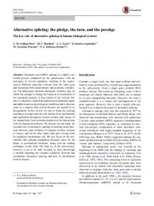
We used five 20 vs 20 DIEGO predictions from the time and memory benchmark series above to investigate whether the distribution of splice sites deemed differentially used by DIEGO is different to the background distribution with respect to the number of splice sites the genes of origin of these splice sites contain. As can be seen in Figure S1, the density of reported splice sites follows the background quite well, with a slight bias to wards genes with more splice sites.

1.4

Input and output formats

DIEGO operates on a tab separated input file that contains information on location, read counts for every data set used and the gene the splice site belongs to. While the preparation of such a file is quite straight forward, we provide scripts to generate these files out of the junction files provided by STAR or the new versions of segemehl, bam files generated by segemehl as well as, for differential exon usage, count files computed by HTseq count (Anders et al., 2015) (as used in DEXSeq(Anders et al., 2012)). These scripts need a file describing name and location of the data-sets to use as an input. DIEGO also needs a file that maps group information to the names of the data set. DIEGO output consists of a tab seperated file including a header, with columns showing junction identification (usually chromosome:start-stop), junction type (e.g. circular, normal), abundance change, p-value, adjusted p-value, identifier of the gene the junction was assigned to, gene name, number of junctions within the gene, number of significant junctions within the gene, distance of the centers for the gene, a verdict wether DIEGO deemed the result significant (yes/No), information about whether or not zero replacement had to be performed on the junction (True/False).

References Anders, S., Pyl, P. T., and Huber, W. (2015). Htseq–a python framework to work with high-throughput sequencing data. Bioinformatics (Oxford, England), 31(2):166–169. Anders, S., Reyes, A., and Huber, W. (2012). Detecting differential usage of exons from RNA-seq data. Genome Res., 22(10):2008–2017.

Background 1 2 3 4 5

0.02 0.00

0.01

density

0.03

0.04

Differential Differential Differential Differential Differential

0

10

20

30

40

50

60

number of splice sites per gene

Supplemental Material, Figure S1: Density of DIEGO reported differentially used splice site on number of splice sites in gene of origin (coloured curves) vs. background distribution (black area).

Benjamini, Y. and Hochberg, Y. (1995). Controlling the false discovery rate: A practical and powerful approach to multiple testing. J. R. Stat. Soc. Series B Stat. Methodol., 57(1):289–300. Cancer Genome Atlas Network (2012). Comprehensive molecular portraits of human breast tumours. Nature, 490(7418):61–70. Dobin, A., Davis, C. A., Schlesinger, F., Drenkow, J., Zaleski, C., Jha, S., Batut, P., Chaisson, M., and Gingeras, T. R. (2013). Star: ultrafast universal rna-seq aligner. Bioinformatics (Oxford, England), 29(1):15–21. Kretzmer, H., Bernhart, S. H., Wang, W., Haake, A., Weniger, M. A., Bergmann, A. K., Betts, M. J., Carrillo-de Santa-Pau, E., Doose, G., Gutwein, J., Richter, J., Hovestadt, V., Huang, B., Rico, D., J¨ uhling, F., Kolarova, J., Lu, Q., Otto, C., Wagener, R., Arnolds, J., Burkhardt, B., Claviez, A., Drexler, H. G., Eberth, S., Eils, R., Flicek, P., Haas, S., Hummel, M., Karsch, D., Kerstens, H. H. D., Klapper, W., Kreuz, M., Lawerenz, C., Lenze, D., Loeffler, M., L´ opez, C., MacLeod, R. A. F., Martens, J. H. A., Kulis, M., Mart´ın-Subero, J. I., M¨ oller, P., Nagel, I., Picelli, S., Vater, I., Rohde, M., Rosenstiel, P., Rosolowski, M., Russell, R. B., Schilhabel, M., Schlesner, M., Stadler, P. F., Szczepanowski, M., Tr¨ umper, L., Stunnenberg, H. G., ICGC MMML-Seq project, BLUEPRINT project, K¨ uppers, R., Ammerpohl, O., Lichter, P., Siebert, R., Hoffmann, S., and Radlwimmer, B. (2015). DNA methylome analysis in Burkitt and follicular lymphomas identifies differentially methylated regions linked to somatic mutation and transcriptional control. Nature genetics, 47(11):1316– 1325. Li, B. and Dewey, C. N. (2011). Rsem: accurate transcript quantification from rna-seq data with or without a reference genome. BMC bioinformatics, 12:323. Mann, H. B. and Whitney, D. R. (1947). On a test of whether one of two random variables is stochastically larger than the other. Ann. Math. Stat., 18(1):50–60.