Diffeomorphic Registration of Images with Variable ... - Semantic Scholar

Diffeomorphic Registration of Images with Variable Contrast Enhancement Guillaume Janssens1 , Laurent Jacques1 , Jonathan Orban de Xivry1 , Xavier Geets2 , and Benoit Macq1 1 2

Information and Communication Technologies, Electronics and Applied Mathematics (ICTEAM), Department of Radiation Oncology, Laboratory of Radiobiology and Radiation Protection (RBNT), Université catholique de Louvain (UCL), Belgium.

September 28, 2010

Abstract

speed [6, 7, 8]. Besides, the choice of a registration method for medical application depends on the characteristics (e.g., modality) of the images to be registered [1]. The existing methods [9] can be divided into parametric, or model-based, methods (Bsplines[10], thin-plate splines[11], radial basis functions[12], linear elastic FEM [13], etc.) and non-parametric methods (viscous fluid[14], optical flow[15], etc.). In this second category, the algorithm called Demons [16, 17] is fast, efficient and easyto-use, as it requires no particular pre-processing nor patientspecific modeling. This method aims at calculating a regular displacement field which produces a good matching of the intensities in both images by minimizing a metric, such as the sum of squared differences (SSD) [18] or the mutual information (MI) [8], between images along with a measure of the field regularity. In a growing number of applications, the displacement fields resulting from registration are used to deform images from other modalities or other spatial distribution maps (e.g., the dose map associated to CT scans in radiotherapy [19, 20]). Therefore, the matching of structures in images based on their intensities is not a sufficient constraint for producing realistic anatomical deformation estimations [21]. This is the reason why a priori information on the physical characteristics of anatomical deformations have to be included in the registration process. Diffeomorphism is a necessary condition for displacement fields to be physical [22]. Indeed, organs can be compressed and deformed, but cannot undergo non-invertible spatial transformations, e.g., showing mirror effects. A method has been proposed in [23] to limit the displacement fields computed by the Demons to a set of diffeomorphic transformations, using diffeomorphic flows and Lie algebra. In several medical protocols, contrast agents are used in order to facilitate interpretation. This makes the registration problem incompatible with the hypothesis of intensity conservation. Furthermore, an histogram equalization is often not able to correct for contrast agent variability, as different regions will be enhanced in different ways inside the image. Therefore, simple metrics, such as SSD or cross-correlation, are not suitable for matching those images, and methods that are suitable for registering variable contrast images have to be investigated [24, 25]. A method similar to Demons but using a phase-based approach was first proposed in [26], and was called Morphons.

Non-rigid image registration is widely used to estimate tissue deformations in highly deformable anatomies. Among the existing methods, non-parametric registration algorithms such as optical flow, or Demons, usually have the advantage of being fast and easy-to-use. Recently, a diffeomorphic version of the Demons algorithm was proposed. This provides the advantage of producing invertible displacement fields, which is a necessary condition for these to be physical. However, such methods are based on the matching of intensities and are not suitable for registering images with different contrast enhancement. In such cases, a registration method based on the local phase like the Morphons has to be used. In this work, a diffeomorphic version of the Morphons registration method is proposed and compared to conventional Morphons, Demons and diffeomorphic Demons. The method is validated in the context of radiotherapy for lung cancer patients, on several 4D respiratorycorrelated CT of the thorax with and without variable contrast enhancement. Keywords : Non-rigid image registration, diffeomorphism, Morphons, contrast enhancement, lung cancer.

1 Introduction In the context of image-based medical diagnostics and treatment, highly deformable anatomies are a problem for multiple time imaging analysis along the course of treatment. Indeed, a precise tracking of organs is made difficult because of shape and position variations. Non-rigid registration may be used to compute a displacement vector for each voxel of an image [1], enabling the estimation of the spatial variations of the anatomy. The displacement vectors are computed as pointing to the best corresponding location of the voxels in another image according to a metric which is a measure of the image matching and under some constraints on global properties of the resulting deformation, such as invertibility and smoothness. Several registration methods have been used in the past years to estimate deformations in highly deformable anatomies [2, 3, 4, 5]. Many efforts have been made to improve the quality of displacement estimates, but also to reduce the amount of required pre-processing or modeling and improve registration 1

e.g., for two displacement fields D1 and D2 , D1 ⋄ D2 = D1 ◦ ∆2 . In practice, the warping is applied on discrete images. The transformation might therefore need to be truncated (on the volume boundaries) to the closest point inside the volume in order to avoid extrapolation of the images to be warped.

The principle of the method is to match transitions (between dark and bright zones) rather than intensities, by looking locally at the spatial oscillations in intensities. This method uses Gaussian smoothing as regularization of the displacement field and additive accumulation during the iterative process. This is nevertheless not sufficient to ensure the invertibility of the deformation [29, 22]. In this paper, a Morphons registration using a diffeomorphic accumulation step is proposed and its accuracy is assessed in the case of thorax image registration, also in presence of different contrast enhancements, and compared to the Demons. The paper is organized as follows. In Section 2, the main mathematical concepts and definitions are presented. Then in Section 3 a generic non-parametric registration process is presented and its particularization to Morphons and to diffeomorphisms is proposed in Section 4. In Section 5, different registrations are applied on images of the thorax, without contrast enhancement in the first experiment, and with contrast enhancement in the second. The results of these experiments are eventually discussed in Section 6.

2.2

Compositive Accumulation

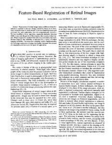
In this paper, we promote a particular way to combine, or accumulate, properly two displacement fields D1 and D2 . Adding them to form D1 + D2 (as performed by many non-parametric registration methods, see Section 3), is of course computationally efficient, but it breaks the consistency with the composition of the corresponding spatial transformations, as illustrated in Fig. 1.

2 Mathematical Framework

(a) D2

(b) D1

(c) D1 ⋄ D2

For the sake of clarity, let us introduce some key mathematical concepts used throughout this paper.

2.1

Images and Deformation Fields

In this paper, we always denote 3D images by lower case let(d) x + D2 (e) x + (D1 + D2 ) (f) x + (D1 ⊕ D2 ) ters. For instance, in the process of estimating a displacement field, the fixed and the moving images are written f and m respectively. We consider them as real valued functions on the volume R3 of points x = (x1 , x2 , x3 ), i.e., f , m ∈ F = {g : R3 → R : x 7→ g(x)}. Most of the time, these functions, but also the continuous operations performed on them, such as convolutions or integrals, must be understood as approximated on the dis(g) moving image m (h) m ⋄ (D1 + D2 ) (i) m ⋄ (D1 ⊕ D2 ) crete voxel grid G = {(x1 , x2 , x3 ) ∈ Z3 }, omitting the treatment of volume boundaries. In this study, image convolutions were Figure 1: Comparison between additive and compositive field performed using zero-padding outside the boundaries. accumulations. Warping is implemented using linear interpoA displacement field on R3 is a vectorial field D ∈ V = lation. In (a) and (b), two different displacement fields are de{V : R3 → R3 , x 7→ V (x)}. It is associated to the “deformation” fined on the plane (for visual clarity). In (c), the field D1 warped operation ∆ , Id +D, i.e., ∆(x) , x + D(x), with Id the identity by D2 , i.e., D1 ⋄ D2 = D1 ◦ ∆2 . In (d), the field D2 is applied on deformation: Id(x) , x. The operation ∆, and by extension its the pixel grid. In (e), the grid is warped by the field resulting vector field D, is said diffeomorphic if it is invertible, differen- from an addition-based accumulation of D1 and D2 . In (f), the tiable, and its inverse is differentiable. For the transformation grid is warped by the displacement field D1 ⊕ D2 arising by the ∆ to be invertible, its Jacobian must not vanish in any point x, composition of ∆1 and ∆2 , which is the sum of the dark blue i and gray arrows (given by ∆1 ◦ ∆2 − Id). This composition is that is, if det(J )(x) 6= 0∀x, with J i j = ∂∆ ∂x j . Moreover, it has to be positive (det(J )(x) > 0). Indeed, a transformation ∆ with neg- really the accumulation that matters since it corresponds to the ative Jacobians does not correspond to physical deformations way displacement fields are iteratively applied to an image (see Section 3). Since D1 ⊕ D2 = D2 + D1 ⋄ D2 , the summed vectors (as the mirror operation). in (f) correspond to the vectors in (a) and (c). In (g), a moving Mathematically, given the images f and m, we will see object m, divided in 4 colors (regions between pixel centers). that our global objective of our study is to estimate D such that In (h), the result of the warping of m by the sum of the fields. the warping of m by D is “close” to f , i.e., f ≃ m ◦ ∆ with ◦ Clearly, the surfaces are inverted (mirror effect, visible because the common function composition. We will use sometimes the of the inversion of colors), leading to non-physical deformanotation tions (negative Jacobians). In (i), the result of the warping of m m ⋄ D = m ◦ ∆, by the composition of the fields. One can notice that, in spite of to insist on the warping action of D on m. By extension, this the deformation of the shape of the object, the location of the warping symbol can also be used on vector fields themselves, colors is conserved. 2

Indeed, one can clearly see in Fig. 1(h) that the warping of the image in Fig. 1(g) by the sum of two diffeomorphic fields, D1 and D2 , does not correspond to the successive warping of this image by D1 and then by D2 , which is represented in Fig. 1(i). However, the compositive operation, denoted ⊕, solves this issue. It is simply defined as

D x D(x) ∆(x) exp(D)(x)

D1 ⊕ D2 , ∆1 ◦ ∆2 − Id .

ϕD (x, t)

By construction, the deformation operation linked to the deformation field D1 ⊕ D2 is therefore ∆1 ◦ ∆2 . If both displacement fields are diffeomorphic, their composition is also diffeomorphic [38]. The operation ⊕ has some interesting and useful properties. First, the neutral accumulation is of course obtained with the null displacement field, i.e., D ⊕ 0 = 0 ⊕ D = D. Second, it is easy to prove the associative relations (D1 ⊕ D2 ) ⊕ D3 = D1 ⊕ (D2 ⊕ D3 ) = D1 ⊕ D2 ⊕ D3 for three displacement fields D1 , D2 and D3 . And finally, ⊕ and ⋄ are linked through the simple relation:

Figure 2: The diffeomorphic flow exp(D) associated to the vector field D is the solution at time t = 1 on the trajectory tangent to D at each point (here represented in 2D). We see that the motion of x induced by exp(D)(x) is more compatible with V than this produced by ∆(x) = x + D(x).

Indeed, when the field D is close enough to zero (i.e., ∆ ≈ Id), the exponential of the field can be approximated using the firstorder Taylor expansion exp(D) ≈ Id +D = ∆, i.e., by the transformation itself. On the other hand, the solution of the flow equation (1) in t = 1 can be approximated by “discretizing” t k between 0 and 1. Indeed, as exp(D) = exp(2−k D)2 (where the k exponent 2 expresses the number of times the deformation operation is combined with itself), one can use the scaling and squaring strategy for computing the exponential [30]. If one chooses k such that the field 2−k D is close enough to zero, the first-order approximation can be used to estimate exp(2−k D) (based on the Padé approximant near the origin). Then the solution of the flow equation is computed by performing k recursive compositions of the field by itself, given that such compositions are computationally affordable. Notice that taking k = 0 is equivalent to the simple first-order approximation. The scaling and squaring steps for field exponentiation [22] is depicted hereafter:

D1 ⊕ D2 = D2 + D1 ⋄ D2 , meaning that the displacement field D1 ⊕ D2 is equivalent to summing the field D2 with the field D1 warped by D2 . This is illustrated in Fig. 1: the vectors in Fig. 1(i), corresponding to the successive warping by D1 and then D2 , are the sum of the vectors in Fig. 1(a) and Fig. 1(c), as shown in Fig. 1(f).

2.3

Diffeomorphic Flow and Exponentiation

An important notion used in Section 4.2 is the concept of (continuous) diffeomorphic flow [27, 28, 29]. Given a point x ∈ R3 and a smooth vector field D ∈ V , the flow ϕD (x,t) is the dynamic solution u(t) ∈ R3 of the following (autonomous) ordinary differential equation: ( d dt u(t) = D(u), (1) u(0) = x.

• Scaling: Divide D by a factor 2k such that 2−k D is small enough, e.g., when k2−k Dk∞ = maxx k2−k D(x)k < 0.5 voxels.

At a given “time” t > 0, the position ϕD (x,t) is simply a point on the trajectory following D tangentially from the initialization on x (see Fig. 2). Following [29], the expo• Exponentiation: Compute first-order explicit integration nential of a vector field D, i.e., exp(D) ∈ V , is the nonof the flow: ∆(0) (x) = ϕD (x, 2−k ) ≈ Id(x) + 2−k D(x). linear deformation operation obtained by the flow of D at time t = 1, i.e., exp(D)(x) = ϕD (x, 1). Interestingly, this exponential map acts as the common scalar valued exponential, • Squaring: Perform k recursive squarings (using field comi.e., exp(αD) ◦ exp(βD) = exp((α + β)D) for α, β ∈ R, and position) of the flow at time 2−k in order to obtain the it is invertible by simply considering the inverted vector field, flow at time 1, which is the field exponential. In other i.e., exp(−D) ◦ exp(D) = Id. In addition, for differentiable D, words, starting with ∆∗ = ∆(0) , do k times the computa3 exp(D) is also a diffeomorphism on R . In other words, exp(D) tion ∆∗ ← ∆∗ ◦ ∆∗ , in order to get ∆∗ ≃ exp(D). modifies the 3D coordinates with no intersection between the motions of points. Indeed, such a possibility would induce a point x with two different motion vectors, a situation that is We see that using this method, only k compositions (and thereforbidden by (1) since D(x) is uniquely defined. fore k interpolations) are needed for estimating the exponential. Compared to standard estimation of the flow over a regular discretization of the time interval [0, 1] in 2k steps, the scaling and 2.4 Scaling and Squaring squaring method limits the numerical errors due to composition A numerical scheme exists to compute approximately but effi- of vector fields, but it does not decrease the amplification of the ciently exp(D)(x) when x belongs to a regular grid of voxels G . error due to the field estimation at time t = 2−k . 3

3 Generic Registration Pipeline

Moving image Image warping

Non-rigid registration methods can be divided into parametric and non-parametric methods. Parametric (or model-based) methods aim at calculating the parameters of a deformation model in a high-dimensional space in order to optimize a global objective function that takes into account image similarity and transformation regularity [10]. In this case, the a priori information is included in the modelization and regularity criteria of the non-rigid transformation. For example, the harmonic energy of transformation can be explicitely included in the objective function [31]. On the other hand, non-parametric methods makes it possible to decouple similarity optimization from regularization by directly acting on the displacement field. The a priori information has then to be included in the optimization process by using proper regularization techniques. Decoupled optimization makes the registration computationally efficient [8], mainly because the computation of each displacement vector is independant from others, but it prevents us from easily including more complex regularization constraints in the process, e.g., such as in volume preserving registrations [32, 33].

Regularization

Coarsest scale

Warped image Finest scale

Fixed image

Update field computation

Accumulation

Figure 3: The non-parametric registration pipeline is composed of 3 main operations (Θ, Φ and Ψ) and the warping of the moving image. Those operations are performed from coarse to fine scales. At each scale, the process is applied iteratively, until it reaches a stopping criterion.

where ∆a and ∆u denote the deformation operations linked to Da and Du respectively. Depending on the nature of the images to be registered, Most non-parametric registrations are based on an iterative pro- this local displacement estimation can be based on different locess which is composed of 3 steps: (i) Field Computation, (ii) cal image metrics, such as SSD [17], mutual information comField Accumulation and (iii) Field Regularization. The idea puted on blocks of voxels [35, 8], local phase [26], etc. is to progressively build a proper displacement field by iteratively improving the matching between the fixed image and the moving image warped by this displacement field, accord- Field Accumulation ing to a certain metric. Note that, depending on the nature of the displacement one tries to model, the regularization is ap- After the field computation, the total displacement Da must be plied either on the increment field or on the accumulated field. increased by the update field: Regularizing the field increment corresponds to a viscous fluid Da ← Φ(Da , Du ). (3) modeling, while regularizing the global transformation corresponds to an elastic solid modeling [14]. Only the second is This accumulation operation Φ is sometimes implemented considered in this study. as a simple addition of accumulated and update fields (as in In this paper, our general non-parametric registration [18], [36] and [37]). However, as explained in Section 2.2, framework (e.g., valide for Demons and Morphons) adopts a this accumulation is perhaps computationally efficient but is multi-scale approach, that is, the displacement field estimation not consistent with the composition of the corresponding spais stabilized by decomposing the fixed and the moving images tial transformations. The solution is therefore to replace it by in several scales, e.g., using a simple smoothing and down- the compositive accumulation ⊕ introduced earlier. The acsampling procedure [34]. cumulation Da ⊕ Du of the displacement fields Da with Du is The three steps mentioned above are then applied a certain then compatible with the way Du is estimated. Indeed, since number of times (until the algorithm reaches a certain stopping Du is computed from m ◦ ∆a , the accumulation of Da and Du criterion) to each scale separately from coarse to fine scales must modify Da by Du , a process intrinsically integrated by (Fig. 3). The general explanation of these three basic blocks the operation ⊕. Moreover, the associativity of ⊕ validates the are given hereafter. The way they are iteratively applied at each compositive accumulation of displacement fields over several scale is described in Section 3.2. iterations, as illustrated in Fig. 3.

3.1

Multiscale Non-Parametric Registration

Field Computation

Field Regularization

At each iteration of the registration process, an update displacement field (Du ) is first computed as a function (Θ) of the fixed image ( f ) and the moving image (m) warped by the displacement field resulting from previous iterations (Da ):

Eventually, the field is regularized in order to get a smoother transformation and reduce the impact of image noise on the registration output: Da ← Ψ(Da ). (4)

Du ← Θ( f , m ◦ ∆a ),

This operation Ψ is achieved by applying a low-pass filter on (2) each components of the displacement field. We assume it to be 4

a Gaussian smoothing with a size σ2Ψ of a few voxels, which Table 1: Multi-scale Non-Parametric Procedure tends to reduce the harmonic energy of the transformation [31]. Inputs and parameters: It is always possible to produce invertible fields by per• Images f and m defined on G . forming a very strong Gaussian smoothing. This, however, may reduce significantly the accuracy of the estimated displacement • Number of scales J. by limiting the solution to excessively smooth displacement • A stopping criterion S . fields. On the other hand, by preventing the displacement field from being non-invertible, the diffeomorphic accumulation acts • Gaussian kernel variance σ2Ψ of Ψ. in some way as a regularization, allowing the estimation of inOutput: The displacement field Da . vertible fields while performing only moderate smoothing. Algorithm:

1. Initialization:

3.2

Set scale to j = J and initialize Da = 0 on G J+1 .

Registration Algorithm

2. Transfer on grid G j : Let us explain now the whole multi-scale non-parametric regCompute m j = Down j (m), f j = Down j ( f ), istration algorithm relying on the three specific procedures and assign Da ← Up(Da ). {Θ, Φ, Ψ} defined in Section 3.1. The algorithm takes as inputs the fixed and the moving 3. While S is false, do: images f and m, some parameters described below, and outputs (i) Warping: w = m j ◦ ∆a the estimated transformation ∆a = Id +Da such that f ≃ m ◦ ∆a . (ii) Field computation: Du ← Θ( f j , w) The whole procedure described in Table 1 and depicted in Fig. 3 involves computations on different scales j ∈ [0, J], from (iii) Accumulation: Da ← Φ(Da , Du ) coarse ( j = J) to fine ( j = 0). Each scale is associated to a j (iv) Regularization: Da ← Ψ(Da ) sub-sampled grid of voxels √ G j = κ G , where κ is the subsampling factor (e.g., κ = 2 in this study) between scale j and 4. If j = 0, stop and return Da , scale j + 1. The functions f and g, defined on the initial grid else, set j ← j − 1 and return to step 2. G = G 0 = {(x1 , x2 , x3 ) ∈ Z3 }, are down-sampled (after antialiasing smoothing) at any scale j by the operation Down j (). An up-sampling operator Up(), implemented as a simple linear mation Θ is actually split into two quantities, interpolation, is used to transfer any displacement field defined Du ← ΘD ( f , w) on a grid G j+1 to the finer grid G j using κ as up-sampling factor. For each scale j ∈ [0, J], the accumulated displacement cu ← Θc ( f , w), field is iteratively updated until one reaches a particular stopping criterion S (e.g., based on the convergence of Da or on the that is, respectively, an update of the displacement field along with an update of the certainty map. A similar split is also SSD, as precised in Section 5). performed on subsequent operations Φ and Ψ. Here are the details about the three steps {Θ, Φ, Ψ} of the pipeline of Section 3 for this specific registration, including our contribution to the field accumulation step. 4 Diffeomorphic Morphons

4.1

Our paper adapts the global registration method explained in the previous section to Morphons [26, 39] by taking care of the invertibility of the accumulated displacement field, that is, by introducing diffeomorphic field accumulations. As already mentioned above, the particularity of Morphons, compared to other non-parametric methods, is that the field computation (function Θ in Equation 2) is based on the local phase rather than intensity difference. In other words, knowing the phase difference between periodic signals of the same frequency allows the estimation of the spatial shift between them. Therefore, under the assumption that images can locally be considered as a sum of periodic signals, the computation of the local phase difference is equivalent to the estimation of the local displacement between images. This procedure is stabilized by the multi-scale approach described in Section 3.2. Besides, Morphons combines the estimation of displacement vectors with a measure of the confidence we have in these estimations, resulting in a certainty map. Therefore, for Morphons, given two images f and w = m ◦ ∆, the displacement field esti-

Displacement Field Calculation

In Morphons, a displacement field is estimated thanks to the dephasing between the local phases of the fixed and the moving images. This local phase can be probed at a certain frequency and in a particular direction using quadrature filters [40]. More precisely, Morphons method uses a quadrature filter hη of direction η ∈ R3 (also called loglets [40]) defined in frequency by the polar separable function b )2 R(kωk), Hη (ω) = χ+ (ηT ω) (ηT ω

where ω ∈ R3 is the frequency vector, χ+ (λ) = 1 if λ > 0 and b = ω/kωk is the unit vector supporting 0 else, kωk2 = ωT ω, ω ω and R is a radial function centered on ρ > 0 and defined as R(r) = exp[− ln2 (r/ρ)/ ln 2 ] for r > 0. Since their support corresponds to the half volume {ω ∈ b )2 = cos2 φ (with φ the angle R3 : ηT ω > 0} and since (ηT ω separating ω and η), loglets can be seen as the analytic counterparts of the steerable filters introduced by Freeman and Adelson 5

Jointly to the estimation (Equation 5), a global certainty map associated to the quality of the estimation of ΘD is defined as [43] Θc ( f , w) = ∑ ck (x),

[41]. As a matter of fact, only a limited number of orientations η are necessary to cover the whole frequency plane. Typically, in 2-D, these directions are taken as ηk = (cos φk , sin φk ) with φk = kπ/4 for 0 ≤ k ≤ 3, and in 3-D, η is taken as the 6 normal vectors {ηk : 0 ≤ k ≤ 5} to the faces of a hemi-icosahedron [42, 43]. Notice also that each filter hk (x) in the spatial domain is centered around the origin with a typical width given by 1/ρ. Morphons take advantage of the following behavior. Given an image f , defining the filtering

k

i.e., the sum of all certainty measures for each quadrature filter. This update of the certainty map must then be combined with an accumulated certainty computed from previous iterations (see Section 4.2). In the multi-scale approach described in Section 3.2, using the same quadrature filters at decreasing scales Hηk is equivalent to estimating the phase of the band-pass filtered image around increasing cut-off frequencies, that is, with ρ ← 2ρ each time j ← j + 1. This sustains the coarse-to-fine displacement estimation, that is, the computation of ΘD and Θc on different scale bands f j and m j of f and m. Convolutions with quadrature filters can be implemented efficiently in the Fourier domain thanks to the FFT and the convolution theorem. However, since the spatial extent of those filters is small, it is also possible to use efficient spatial convolutions with truncated kernels, as done in this study. As the local phase is invariant to local intensity scaling, the Morphons procedure is suitable for registering images with various contrast enhancements. Besides, some studies indicate that the phase extraction allows a fast convergence and a sub-voxel precision in displacement estimation (e.g., see [39]).

q f (x; k) = ( f ∗ hk )(x), with ∗ the common convolution operation and the shorthand hk = hηk , we can write q f (x; k) = A f (x; k) eiφ f (x;k) since q f ∈ C. Therefore, by processing the warped image w similarly, the local phase difference can be computed as
∆φk (x) = arg q f (x; k) q∗w (x; k) ,

with (·)∗ the complex conjugation and ∆φk (x) = φ f (x; k) − φw (x; k) the local dephasing between f and w in direction ηk . An important observation is that the non-negative value Z f (x′ ) Tx hk (x′ ) dx′ , A f (x; k) = |( f ∗ hk )(x)| = R3

represents also the correlation between f (x′ ) and the translated filter Tx hk (x′ ) = hk (x′ − x), that is, the filter hk (x′ ) = hk (−x′ ) translated on x. If the image f was perfectly represented by the latter, that is, if we had locally f (x′ ) = c hk (x′ − x) for any x′ ∈ R3 and some constant c ∈ R, a displacement of f by a displacement field D(x) approximately constant over the support of Tx hk would induce a dephasing ∆φk (x) = ρηTk D(x) since the frequency vector of Tx hk is −ρηk . An important implicit assumption is nevertheless that |ρηTk D(x)| < π since the dephasing is known up to modulo 2π. Moreover, only ηTk D and not D can be determined, as another manifestation of the blank wall problem [44]. In practice, for most of x, f (x) is not perfectly represented by one filter but by a linear combination of them where the amplitude A f (x; k) measures the adequacy of the fit between f (x) and Tx hk . Consequently, the local update displacement Du (x) linking f (x) and w(x) = f (x + Du (x)) in each x ∈ R3 is estimated by solving the weighted least square optimization 
2 ΘD ( f , w) = arg min ∑ ck ρ ηTk d − ∆φk , (5)

In the original Morphons method, the accumulated field is computed as a weighted sum of the update field and the previous accumulated field, as used in damped optimization schemes. The weights are given by the certainty on the update field (cu , as computed from Θc ) and the accumulated certainty map (ca ). As the certainty map must also be accumulated in order to reflect the confidence in all previous displacement computations, the accumulation step Φ must be divided into two operations ΦD (field accumulation) and Φc (certainty accumulation):

with ΘD ( f , w) arbitrary set to 0 when (N T C2 N) is not invertible.

der to limit the possible solutions to diffeomorphic transformations. In practice, this is done by replacing the accumulation

d∈R3

4.2

Field Accumulation

u Du , ΦD (Da , Du , ca , cu ) = Da + cac+c u

Φc (ca , cu ) =

c2a +c2u ca +cu ,

(6) (7)

where in the last formula, similarly to the field accumulation, where the ck (x) = A f (x; k)Am (x; k) are the certainty map of the the certainty map is updated by its own certainty [43]. However, as it was explained before, the addition of disfilter hk . As explained above, ck reflects for each voxel how placement fields is not really appropriate for accumulating spareliable the field estimation is, i.e., how contrasted the bandtial transformations, in contrast to composition. The composipass filtered images are. tive accumulation may also be damped using the certainty as a Numerically, the optimization in Equation 5 is a stanweighting factor: dard weighted least square minimization, that is, it corresponds the minimization of the energy E(d) = kC(Nd − Γ)k22 , usu Du . ΦD (Da , Du , ca , cu ) = Da ⊕ cac+c u ing the diagonal matrix C = diag(c1 , · · · , c6 ), the matrix N =
T (η1 , · · · , η6 )T and the vector Γ = ∆φ1 , · · · , ∆φ6 . An easy The (SSD-based) Demons registration is a non-parametric computation shows that the solution of (5) is then given by the algorithm which performs the optimization of the SSD between † T 2 −1 T Moore-Penrose pseudo inverse (CN) = (N C N) N C, that images. In [29], a diffeomorphic field accumulation is proposed is, as improvement of the Demons method. The idea is to use an ΘD ( f , w) = (CN)†C Γ, adaptation of the optimization method to Lie groups [45] in ork

6

step of the Demons by an accumulation using the diffeomorphic flow exp() introduced in Section 2. This accumulation reads then
ΦD (Da , Du ) = Da ⊕ exp(Du ) − Id , (8)

This operation tends to propagate the displacement field from high certainty areas to areas which show less significant filter responses. Besides, by setting to zero the certainty outside the volume boundaries, normalized convolution cancels the influence of the padding strategy. This step produces a smooth version of the accumulated field that may reduce the accuracy of image matching resulting from the displacement estimation step, as it limits the possible solutions to smooth displacement fields. However, if the iterative algorithm is to converge, the solution will be regular and invertible (except for large numerical errors), thanks to accumulation and regularization constraints, but it will also be (at least locally) optimal in terms of local phase difference. Indeed, as the phase is monotonic and smooth, a mismatch between local structures will automatically lead to non-zero field update with a high certainty value, which will tend to improve the displacement estimate and fit the structures together. The Jacobian of the displacement field may be used as a criterion for validating the physical behavior of the deformation. Indeed, the Jacobian gives for each voxel the change in volume this voxel encounters during deformation. Jacobian indicates expansion when it is greater than 1, and compression when it is smaller than 1. A negative Jacobian means that the voxel is “inverted” (getting a negative volume), which is incompatible with the mass-preservation principle. In the following, the diffeomorphic version of Demons and Morphons are denoted respectively D-Demons and DMorphons.

where the field exponential exp(Du ) can be efficiently estimated using a small number of recursive compositions of the field Du by itself. Consequently, the displacement field ΦD (Da , Du ) is linked to the deformation operation ∆a ◦ exp(Du ). In the case of the Morphons, the accumulation step can be achieved in the same way. This will produce smoother fields than the traditional addition or composition. However, the accumulation step in the Morphons method involves a damping based on the certainty. Therefore, we propose the following accumulation step for diffeomorphic Morphons:
u Du ) − Id . (9) ΦD (Da , Du , ca , cu ) = Da ⊕ exp( cac+c u

Since exp(0 D) = Id for any vector field D, the accumulation fades away when ca ≫ cu . The accumulation of the certainty map remains as explained previously (Equation 7). Notice that, because the field is discretized on a grid of voxels, interpolation is needed for computing the composition of two diffeomorphisms. Therefore, errors due to successive interpolations could potentially lead to non-invertible transformations. However, such problems were not observed in practical experiments using reasonable smoothing of the field.

4.3

Field Regularization

5 Experiments and Results

During the displacement estimation step, the relevance of local phase computation is estimated and used as weight for the accumulation. This certainty map may also be used for a smart regularization of the displacement field. Regularization is performed using a normalized convolution [46] of the field by a Gaussian kernel, taking into account the certainty map in order to put greater importance to high certainty locations. The certainty is also regularized in the same way as displacement field components in order to preserve the correspondence between the displacement vectors and their corresponding certainty. Mathematically, given a positive function h and a filter g (typically a Gaussian kernel of variance σΨ > 0), the normalized convolution of a (scalar) function s by g as involved by the normalization h is

The methods were first compared for several simple 2D virtual situations in order to demonstrate the interest in chosing the accurate registration method with respect to the images to be registered. For the clinical validation, Morphons and D-Morphons registrations were first validated on a 10-phases point-validated pixel-based breathing thorax model (POPI-model) from the Léon Bérard Cancer Center, Lyon, France [4] in order to compare the D-Morphons to Morphons, Demons and D-Demons in the case of intensity conservation between images. Then it was applied to lung images with different contrast enhancements, in order to illustrate the benefit of a phase-based approach compared to traditional SSD-based registration methods in the case (h s) ∗ g where intensities are not conserved between the images to be . s ∗h g , h∗g registered. All simulations were performed using Linux, on a single This operation does not increase the maximum amplitude of the R

filtered function. Indeed, for a non-negative kernel g, we show processor Intel Core 2 (2.4GHz). Our MATLAB implemeneasily that ks ∗h gk∞ ≤ ksk∞ , with ksk∞ = maxx |s(x)|. The ac- tation used for the prototyping of the methods was also used cumulated displacement field Da and subsequently the certainty for simulation. Notice that no efforts were made for achieving map are therefore regularized thanks to this operation using for good performances in terms of computational cost and memory requirements in the implementations used in this study. The lonormalization the certainty map ca , that is, cal phase estimation was performed using convolutions with ΨD (Da , ca ) = Da ∗ca g, 9 × 9 × 9 quadrature filters. Less than 1 GB of RAM was required for registering two volumes of 256 × 256 × 100 voxels Ψc (ca , ca ) = ca ∗ca g. using all registrations. The time required for registering such Notice that, for computing ΨD , the normalized convolution is images, using the parameters presented hereafter, was around 6 minutes for Demons, 42 for Morphons, 7 for D-Demons and performed separately on all components of the vector field. 7

43 for D-Morphons. However, preliminary results based on a C++ implementation of the Morphons, which uses operations in the Fourier domain instead of convolutions (as done in our MATLAB implementation) and using 4 threads on a quad-core CPU, allowed a division of the computation time by 50, leading to Morphons registrations taking about one minute for such a typical image size.

Moving image

Fixed image

5.1

Displacement field from Morphons

Displacement field from D-Morphons

minimum Jacobian = -680

minimum Jacobian close to 0

Deformed image from Morphons

Deformed image from D-Morphons

Illustrative Virtual Experiments

Two 2D virtual experiments were performed. The first experiment, illustrated in Fig. 4, is based on a virtual disk image after blurring. Two images of the same disk were created, the only difference being the scale of intensities (multiplication by 0.75). This experiment shows the interest in using a phasebased method (conventional Morphons in this example) while registering identical shapes with different contrasts, compared to an intensity-based method (conventional Demons). The second virtual experiment is based on two images of a disk (see Fig. 5). In the fixed image, a disk of radius r1 + r2 was created, and a hole (disk of radius r2 ) was added in its center. In the moving image, a disk of radius r1 was created with the same intensity scaling as in the fixed image. This example illustrates the case where a structure is missing in one image compared to the other, as it may occur in practice (e.g., the problem of bowel gas in CT images of the abdomen). This experiment illustrates how the diffeomorphic version of the Morphons algorithm can prevent from producing negative volumes after registration, without increasing the smoothing by using a larger Gaussian regularization kernel.

Displacement field from Demons

Figure 5: Results of the registration between 2 images using Morphons and D-Morphons registrations, illustrating the case were a structure (i.e., the bright hole at the center of the fixed image) is missing in the moving image. Both methods lead to deformed images very similar to the fixed image except for the central bright part (because it was not present in the moving image). The diffeomorphic method produced very low but still positive Jacobian values ((J) close to 0) in the center of the disk. Given that the field is defined on the pixel grid of the fixed image, this means that the surface of the central bright part (which disappears in the moving image) corresponds, as expected, almost to a singular point in the moving image. The conventional method, however, produced highly negative Jacobians in the central part, leading to the creation of areas that are “mirrors” of areas in the other image.

5.2

Displacement field from Morphons

Accuracy Assessment on a Breathing Thorax Model

The POPI-model [4] is composed of 10 volumes reconstructed from a 4D Respiration-Correlated CT scan (RCCT) of the thorax, each volume corresponding to a particular phase of an average breathing cycle. 41 landmarks were identified by medical experts in each of the 10 images for registration validation. Conventional Morphons, D-Demons and D-Morphons were applied between a reference phase and the 9 others. For all methods, the number of scales was set to J = 8, with final Deformed image Deformed image Fixed image from Morphons from Demons resolution of 2mm × 2mm × 2mm. The variance of the Gaussian kernel used for regularization was empirically set to twice the voxel size (σ2Ψ = 2 voxels). For this experiment, a minimum of 10 and a maximum of 20 iterations was used at each scale. In between, the iterative process was stopped if the changes, measured in terms of SSD, were inferior to 0.01%. Such a convergence criterion was usually reached before the 20th itFigure 4: Results of the registration between 2 identical-sized eration, supporting the fact that both Demons and Morphons blurred disks with different constrasts, using Demons and Mor- behave like optimization methods. The results were then compared with each other and with phons. In yellow: the contour of the disk. In red: the vector field resulting from the registration. The displacement field re- the results from a conventional Demons algorithm as used in sulting from Morphons was very close to zero. Notice that the [4]. The comparisons were achieved in terms of error in landSSD is actually lower using Demons than Morphons. However, mark position, SSD between images, harmonic energy, and the SSD does not reflect the matching of the shapes, in opposi- minimum Jacobian. tion to the disk contour after warping. • The landmark position error evaluates the ability of the registration in finding the physical motion of organs. Moving image

8

• The SSD between fixed and deformed images is a measure of the image matching according to the assumption of intensity conservation. It is computed as ∑x ( f − m ◦ ∆)2 .

SSD 1

Harmonic energy

Minimum jacobian

0.02

0.5

• The harmonic energy [31, 27] of the displacement field D indicates how regular the field is, and is computed as 2 2 2 1 2 ∑x (k∇D1 k + k∇D2 k + k∇D3 k ).

0.01

• The Jacobian of the field indicates the volume change of each voxel. Recall that negative values of the Jacobian correspond to inverted volumes, which is not acceptable in a physical point of view. The Jacobian is computed as ∂di i det(J ), with J i j = ∂∆ ∂x j = δi j + ∂x j , where δi j is the Kro-

0

−0.5

ith

necker’s delta (δi j = 1 if i = j, 0 else) and di is the component of the displacement field. In practice, the par∂di can be computed using centered finite tial derivatives ∂x j difference approximations.

0

0

Figure 6: Results for the 9 registered phases of the POPI model. Left: boxplots of the SSD before registration (in yellow) and after all 4 registrations . Center: boxplots of the energy of deformation after all 4 registrations. Right: boxplots of the minimum Jacobian after all 4 registrations. From left to right, these registrations are: Demons (light blue), Morphons (light green), Diffeomorphic Demons (dark blue) and Diffeomorphic Morphons (dark green). For each box, the center horizontal line represents the median value, the box goes from the lower quartile to the upper quartile, and the vertical lines represent the most extreme values within 1.5 inter quartile range. The crosses represent outlier values.

The comparisons of landmark position errors (expressed in mm) resulting from the different registrations can be seen in Table 2 with, from left to right, the error in landmark position (norm of the difference) before registration, using Demons (values from the POPI website), Morphons, D-Demons and D-Morphons. Position errors are noted as follows: mean / std (max). On average, for Morphons, D-Demons and DMorphons, the error in landmark position was equal or inferior to 1mm, which is half the size of the voxels at the finest scale of the registration process. Results showed that all registrations greatly improved the matching of intensities. The SSD between fixed and deformed image was similar for Morphons, D-Demons and D-Morphons (see Fig. 6). The harmonic energy of the fields resulting from these registrations were also comparable (see Fig. 6). The matching and the harmonic energy obtained by Demons (as presented by the authors of [4] on the POPI website) was slightly less good than for the 3 other methods. However, this is most likely due to the parameters used for registration (e.g., the number of scales, the variance for smoothing, etc.). In particular, for very similar images (first 2 phases of the RCCT), the algorithm was not able to find a smooth displacement field that reduced the SSD. The minimum Jacobian of the displacement fields resulting from conventional methods gets down to -0.5 for both Demons and Morphons (see Fig. 6), as respectively 67 and 460 voxels were inverted for the corresponding phase when applying the field on the moving image (which is composed of almost 6 mega voxels). However, when using diffeomorphic accumulation, the minimum Jacobian was raised to 0.2 for the Demons and 0.1 for the Morphons, showing that the diffeomorphic accumulation step prevented the field from inverting voxels.

i.e., the Internal Target Volume) can be estimated, integrating thus all tumor positions through the respiratory cycle [20]. However, the lack of contrast-enhancement, as well as the high noise level and the presence of artifacts that characterize 4D RCCT, may significantly impair the accurate delineation of the target volumes on these images. More particularly, the iodine contrast agent is of prime importance to help at differentiating tumor extents from vascular structures in the centrallylocated lung tumors. In this context, the acquisition of a conventional contrast-enhanced CT (CE-CT) acquired during free breathing should be considered for the delineation task, while the 4D RCCT is used to estimate the motion range of the tumor during breathing. To automatize this process, the delineated tumor volume at the CE-CT can be deformed on the various respiratory phase images from the 4D RCCT using non-rigid registration to finally get the ITV, as illustrated on Fig. 7. The purpose of this experiment is to compare Demons and Morphons algorithms (conventional and diffeomorphic versions) for the registration between images with and without contrast-enhancement, while keeping the same setting as for the POPI experiment. A CE-CT scan of 3 lung cancer patients was acquired as well as a 4D RCCT scan at another time point. The first CT 5.3 Application to Images of the Thorax with scan was taken in free breathing using an iodine contrast agent. The 4D RCCT scan was acquired without any contrast agent and without Iodine Contrast Agent and was reconstructed into 10 phases. Histogram equalization The breathing-correlated motion of tumor is a typical feature was not able to correct for localized contrast differences beof lung cancer that has to be dealt with in radiotherapy plan- tween the CE-CT and RCCT phase images. For all 3 patients, ning. RCCT images provide information about the tumor mo- Demons, Morphons, D-Demons and D-Morphons were applied tion throughout the breathing cycle. From the different respi- between each of the 10 RCCT images and the CE-CT, with the ratory phases, an adequate margin around the tumor (the ITV, same registration parameters as for the POPI simulation. 9

RCCT phases Phase 1 Phase 2 Phase 3 Phase 4 Phase 5 Phase 6 Phase 7 Phase 8 Phase 9 All phases

Table 2: Results for the POPI experiment: error in landmark position Original Demons [4] Morphons D-Demons D-Morphons 0.5 / 0.5 (2.4) 1.3 / 0.3 (1.8) 0.7 / 0.3 (1.6) 0.7 / 0.3 (1.6) 0.7 / 0.3 (1.6) 0.5 / 0.6 (2.6) 1.4 / 0.2 (2.1) 0.7 / 0.4 (2.1) 0.7 / 0.4 (1.6) 0.7 / 0.4 (2.1) 2.2 / 1.8 (6.6) 1.4 / 0.4 (2.3) 1.2 / 0.6 (2.5) 1.2 / 0.6 (2.5) 1.2 / 0.6 (2.4) 4.3 / 2.5 (10) 1.2 / 0.4 (2.3) 1.0 / 0.4 (2.2) 1.0 / 0.5 (2.5) 1.0 / 0.4 (2.2) 5.8 / 2.6 (12) 1.3 / 0.5 (2.6) 1.1 / 0.5 (2.7) 1.1 / 0.5 (2.5) 1.1 / 0.5 (2.8) 6.1 / 2.9 (14) 1.1 / 0.4 (2.0) 1.0 / 0.5 (2.1) 1.1 / 0.6 (2.8) 1.0 / 0.5 (2.1) 5.0 / 2.3 (12) 1.3 / 0.5 (2.4) 1.1 / 0.6 (2.8) 1.2 / 0.6 (2.7) 1.1 / 0.6 (2.8) 3.7 / 1.6 (6.2) 1.1 / 0.3 (1.7) 0.8 / 0.4 (1.9) 0.8 / 0.4 (1.8) 0.8 / 0.4 (1.8) 2.1 / 1.1 (4.5) 1.1 / 0.3 (1.9) 0.8 / 0.4 (2.0) 0.8 / 0.4 (1.7) 0.8 / 0.4 (2.0) 3.3 / 2.0 (14) 1.2 / 0.4 (2.6) 0.9 / 0.5 (2.8) 1.0 / 0.5 (2.8) 0.9 / 0.5 (2.8) Harmonic energy

Phase 1

0.12

Minimum jacobian 0.5

D1

Phase 2 Reference phase

0.09

0

D2

Reference phase 0.06

Phase 3

−0.5

D3 0.03

Phase 4 D4 0

−1

Figure 8: Results for the variable contrast experiment on 30 phases (3 patients with 10 phases each). Left: boxplots of the energy of deformation after all 4 registrations. Right: boxplots of the minimum Jacobian after all 4 registrations. From left to right, these registrations are: Demons (light blue), Morphons (light green), Diffeomorphic Demons (dark blue) and Diffeomorphic Morphons (dark green). For each box, the center horizontal line represents the median value, the box goes from the The the displacement fields resulting from these registra- lower quartile to the upper quartile, and the vertical lines reptions were compared in terms of harmonic energy and mini- resent the most extreme values within 1.5 inter quartile range. mum Jacobian (see Fig. 8). The resulting image were com- The crosses represent outlier values. pared in terms of SSD and mutual information. The harmonic energy of displacement fields resulting from Demons and D-Demons was quite higher than with the Mor- in terms of mutual information were observed between images phons and D-Morphons, and the minimum Jacobian of the dis- resulting from the different registrations. This is likely due to placement fields were positive only for registrations using the the very low contrasts in the non-contrasted images within the diffeomorphic accumulation. In the worst case, 7455 and 1114 regions corresponding to contrast-enhanced tissues in the other voxels were inverted using respectively Demons and Morphons image, whereas the main differences in terms of displacement without diffeomorphic accumulation (on an image of 5 mega field were located in these regions, as illustrated in Fig. 10. voxels). An example of area leading to bad transformations In order to illustrate the effect of the registration on (with negative Jacobians) using conventional methods is de- contrast-enhanced tissues, one phase of the RCCT scan of one picted in Fig. 9. D-Morphons lead to the smoothest transfor- of the 3 patients was chosen as example. For this patient, the tumation, with minimum Jacobian values around 0.2. These quite mor was located close to contrasted tissues. The tumor and the low values, however, were very sporadic within the image vol- blood vessels were delineated by a physician, on the contrastume. enhanced scan and on one phase of the RCCT scan. The deWe noticed that, unlike the results obtained with the lineations on the phase image were deformed according to the POPI simulation, the SSD resulting from the Morphons and fields resulting from the different registrations. The results are D-Morphons was a bit higher than the SSD resulting from illustrated in Fig. 10. Demons and D-Demons. However, as illustrated in the examThe change in volume due to warping was computed, as ple of Fig. 4, the SSD does not reflect the matching in variable well as the harmonic energy inside the delineated stuctures and contrast areas. On the other hand, no significant differences the difference between the center of mass of the tumor with and Figure 7: Schematic representation of the ITV creation (with only 4 phases). The CTV delineated on a reference image with contrast enhancement (on the left) is deformed towards every phases (middle) using displacement fields estimated by registration and their union is taken as ITV (on the right).

10

tries to match structures of same intensity, which do not correspond to identical anatomical structures because of the difference in contrast agent concentration. Therefore, the field resulting from Demons (see the field on the left part of Fig. 10) is far less smooth than it should be, and can lead to wrong deformation estimations as it illustrated in the example (see Table Fixed image Morphons D-Morphons 3). In this case, the difference in intensity between the images with and without contrast enhancement lead to important volume changes for vessels and tumor by using Demons or DDemons, while almost no changes in volume were observed for these tissues when using a phase-based approach. Besides, the harmonic energy inside these tissues shows that the field is much more smooth using the phase-based registration. It Figure 9: Illustration of negative Jacobians resulting from nonis important to notice that these effects are mostly limited by diffeomorphic registrations. Left: moving and fixed images. the regularization of the displacement field during the Demons Right: fields resulting from registrations (red arrows) and their and D-Demons registrations, and that they will still be worse Jacobian (grayscale images). The negative Jacobians regions if less regularization is used (smaller variance of the Gaussian are contoured in yellow. kernel used for smoothing the displacement field). This is not the case for the fields produced by the Morphons and diffeomorphic Morphons, which are much smoother and preserve the without registration. anatomical topology even with contrast variations between imThe change in volume was very small when using a phase- ages (see Fig. 10). Notice that the reduction of the smallest based field computation for both the vessels (around 0%) and segmentation that can be observed in the Morphons results is for the tumor delineations (around 1%), while it rose up to 23% mostly due to inter-slices motion, as confirmed by the Jacobian for the vessels and to 6% for the tumor while using the Demons. close to 1 in this area that shows that there is no important volIn the same way, the harmonic energy and the error on the cen- ume changes within this segmented region. Finally, one can see ter of mass of the tumor were much smaller for the phase-based that the invertibility of the displacement field is observed with registration methods. These results are summarized in Table 3. both diffeomorphic registrations. These results can be summarized by classifying the difOne can notice that the diffeomorphic accumulation of the field ferent registration strategies according to the smoothness (harin the Morphons did not change the results in terms of harmonic energy) and the invertibility (minimum Jacobian) of the monic energy and volume changes compared to conventional resulting displacement fields (see Table 4) for the variable conMorphons. This is due to the fact that the displacement of the trast experiment. considered organs is small and smooth. Moving image

Demons

D-Demons

6 Discussion

Table 4: Classification of the registration algorithms for variable contrast enhancement.

The first medical experiment showed that D-Morphons and DDemons lead to similar matching of both image intensities and anatomical landmarks. This shows that for mono-modal registration of lung CT scans, the phase difference has an efficiency comparable to the efficiency of the SSD metric. Furthermore, the D-Morphons produced displacement fields as smooth as those obtained with D-Demons. In opposition to conventional Demons and Morphons, both diffeomporphic methods produced invertible displacement fields which are physically meaningful. The second medical experiment illustrates the limitations in registering images with various levels of contrast enhancement with the Demons method. Indeed, the intensity matching resulting from Demons was better than from Morphons, but the field was obviously wrong, as the Demons results in a global shrinking of the contrasted tissues (arteries) that does not reflect a proper anatomical behavior, but that is due to the fact that the Demons registration is based on the minimization of the SSD, which produces an improper displacement estimation when the intensities of identical tissues are different in the fixed and moving images. This mismatch between registered anatomical structures is clearly visible on Fig. 10. As illustrated in the example of Fig. 4, the field produced by Demons 11

Low harmonic energy

High harmonic energy

Invertible (Jmin > 0)

D-Morphons

D-Demons

Non-invertible (Jmin < 0)

Morphons

Demons

One can notice that the D-Morphons algorithm combines both advantages: the field is invertible and smooth, which suggests that it is likely a better estimation of the real transformation which is known to be smooth in this area.

7 Conclusion The D-Morphons is a multi-resolution registration algorithm which computes a diffeomorphic displacement field based on

Table 3: Comparison of volume change, harmonic energy and errors in center of mass of the delineations of the vessels and tumor on a single phase. Original Demons Morphons Volume change (vessels) [in %] Volume change (tumor) [in %] Harmonic energy (vessels) [×10−3 ] Harmonic energy (tumor) [×10−3 ] Error on COM (tumor) [in mm]

23 6 89 39 1.5

2.1

the minimization of the local intensity phase. The method managed to estimate the deformations in a breathing thorax, with an accuracy comparable to the accuracy of the D-Demons, and leads to the same requisite property of invertibility of the field. Moreover, the D-Morphons managed to accurately estimate the deformations between images with variable contrast, while the conventional SSD-based methods lead to misalignment of anatomical structures affected by the contrast variation.

Acknowledgment The authors thank the Medical Informatics laboratory of Linköping University for sharing their implementation of the Morphons. GJ and JOX are funded by a FRIA grant. LJ is a Postdoctoral Researcher funded by the Belgian FRS-FNRS.

0 1 8 4 1.1

D-Demons

D-Morphons

21 6 69 34 1.5

0 1 8 4 1.1

[7] A. Klein, J. Andersson, B.A. Ardekani, J. Ashburner, B. Avants, M.-C. Chiang, G.E. Christensen, L.D. Collins, J. Gee, P. Hellier, J. Hyun Song, M. Jenkinson, C. Lepage, D. Rueckert, P. Thompson, T. Vercauteren, R.P. Woods, J. John Mann and R.V. Parsey, “Evaluation of 14 nonlinear deformation algorithms applied to human brain MRI registration,” in Neuroimage, vol. 46, pp. 786–802, Jan 2009. [8] M. Modat, T. Vercauteren, G.R. Ridgway, D.J. Hawkes, N.C. Fox and S. Ourselin, “Diffeomorphic demons using normalized mutual information, evaluation on multimodal brain MR images,” in Medical Imaging 2010: Image Processing, vol. 7623, 2010. [9] M. Holden,”A review of geometric transformations for nonrigid body registration.”, IEEE Transactions on Medical Imaging, vol. 27, pp. 111-128, Jan 2008. [10] D. Rueckert, L.I. Sonoda, C. Hayes, D.L.G. Hill, M.O. Leach and D.J. Hawkes, ”Nonrigid registration using freeform deformations: application to breast MR images,” IEEE Transactions on Medical Imaging, vol. 18, pp. 712721, Aug 1999.

References [1] J. B. Maintz and M. A. Viergever, “A survey of medical image registration.” Med Image Anal, vol. 2, no. 1, pp. 1–36, Mar 1998.

[11] K. Rohr, H. Stiehl, R. Sprengel, W. Beil, T. Buzug, J. Weese and M. Kuhn, ”Point-based elastic registra[2] H. Wang, L. Dong, J. O’Daniel, R. Mohan, A. S. Gartion of medical image data using approximating thinden, K. K. Ang, D. A. Kuban, M. Bonnen, J. Y. Chang, plate splines,” Visualization in Biomedical Computing, and R. Cheung, “Validation of an accelerated ’demons’ vol. 1131, pp. 297–306, 1996. algorithm for deformable image registration in radiation therapy.” Phys Med Biol, vol. 50, no. 12, pp. 2887–2905, [12] M. Fornefett, K. Rohr, H. Stiehl and Arbeitsbereich KogJun 2005. nitive Systeme, ”Radial basis functions with compact support for elastic registration of medical images,” IVC, [3] A. Pevsner, B. Davis, S. Joshi, A. Hertanto, J. Mechavol.19, pp. 1–2, 1999. lakos, E. Yorke, K. Rosenzweig, S. Nehmeh, Y. E. Erdi, J. L. Humm, S. Larson, C. C. Ling, and G. S. Mageras, [13] M. Ferrant, B. Macq, A. Nabavi and S.K. Warfield, ”Deformable modeling for characterizing biomedical shape “Evaluation of an automated deformable image matchchanges,” Discrete Geometry for Computer Imagery, pp. ing method for quantifying lung motion in respiration235-248, 2000. correlated ct images.” Med Phys, vol. 33, no. 2, pp. 369– 376, Feb 2006. [14] G. E. Christensen, R. D. Rabbitt and M. I. Miller, “Deformable templates using large deformation kinematics,” [4] J. Vandemeulebroucke, D. Sarrut, and P. Clarysse, “The IEEE Transactions on Image Processing, vol. 5, no. 10, popi-model, a point-validated pixel-based breathing thopp. 1435–1447, Oct. 1996. rax model,” in XVth International Conference on the Use of Computers in Radiation Therapy (ICCR), 2007. [15] B. Horn and B. Schunck, ”Determining optical dlow,” MIT Tech. Rep., 1981. [5] E. Rietzel and G. T. Y. Chen, “Deformable registration of 4d computed tomography data.” Med Phys, vol. 33, [16] J.P. Thirion, “Fast Non-Rigid Matching of 3D Medical no. 11, pp. 4423–4430, Nov 2006. Images,” HAL - CCSd - CNRS, 1995. [6] B. Zitova and J. Flusser, “Image registration methods: a [17] J. P. Thirion, “Image matching as a diffusion process: survey,” in Image and vision computing, vol. 21, pp. 977– an analogy with maxwell’s demons.” Med Image Anal, 1000, 2003. vol. 2, no. 3, pp. 243–260, Sep 1998. 12

[18] X. Pennec, P. Cachier, and N. Ayache, “Understand- [30] N. J. Higham, “The scaling and squaring method for the ing the "demon’s algorithm": 3d non-rigid registration matrix exponential revisited,” in SIAM Journal on Matrix by gradient descent,” in Medical Image Computing and Analysis and Applications, vol. 26, pp. 1179–1193, 2005. Computer-Assisted Intervention. Springer, 1999, pp. 597– [31] B. Fischer and J. Modersitzki, “Fast diffusion registra605. tion,” in AMS Contemporary Mathematics, Inverse Prob[19] M. Rosu, I. J. Chetty, J. M. Balter, M. L. Kessler, D. L. lems, Image Analysis, and Medical Imaging, vol. 313, pp. McShan, and R. K. T. Haken, “Dose reconstruction in de117–129, 2002. forming lung anatomy: dose grid size effects and clinical implications.” Med Phys, vol. 32, no. 8, pp. 2487–2495, [32] T. Rohlfing, C.R. Maurer, D.A. Bluemke and M.A. Aug 2005. Jacobs, “Volume-preserving nonrigid registration of MR breast images using free-form deformation with an in[20] J. Orban de Xivry, G. Janssens, G. Bosmans, M. D. compressibility constraint,” IEEE Trans Med Imaging, Craene, A. Dekker, J. Buijsen, A. van Baardwijk, D. D. vol. 22, pp. 730–741, Jun 2003. Ruysscher, B. Macq, and P. Lambin, “Tumour delineation and cumulative dose computation in radiotherapy based [33] E. Haber and J. Modersitzki, “Image Registration with on deformable registration of respiratory correlated ct imGuaranteed Displacement Regularity,” Int. J. Comput. Viages of lung cancer patients.” Radiother Oncol, vol. 85, sion, vol. 71, pp. 361–372, 2007. no. 2, pp. 232–238, Nov 2007. [34] S. Mallat. A wavelet tour of signal processing: The sparse [21] T. Rohlfing, “Transformation model and constraints cause way. Academic Press., 3rd edition, Dec. 2008. bias in statistics on deformation fields.“ Medical image computing and computer-assisted intervention: MICCAI [35] E. Suarez, J.A. Santana, E. Rovaris, C.F. Westin and J. 2006, vol. 9, pp. 207, 2006. Ruiz-Alzola, “Fast entropy-based nonrigid registration,” Computer Aided Systems Theory - EUROCAST 2003, pp. [22] V. Arsigny, O. Commowick, X. Pennec, and N. Ay607–615, 2003. ache, “A log-euclidean framework for statistics on diffeomorphisms.” Medical Image Computing and Computer- [36] L. Ibanez, W. Schroeder, L. Ng, and J. Cates, The ITK Assisted Intervention, pp. 924–931, 2006. software guide second edition updated for ITK version 2.4, Kitware, Ed. Kitware, 2003. [23] T. Vercauteren, X. Pennec, A. Perchant and N. Ayache, ”Non-parametric diffeomorphic image registration with [37] J. Plumat, M. Andersson, G. Janssens, J. O. de Xivry, the demons algorithm,” Int Conf Med Image Comput H. Knutsson, and B. Macq, “Image registration using the Comput Assist Interv, vol. 10, pp. 319–326, 2007. morphon algorithm: an itk implementation,” Insight Journal, 2009. [24] B. Rodríguez-Vila, J. Pettersson, M. Borga, F. GarcíaVicente, E. J. Gómez and H. Knutsson, “3D deformable [38] J. Ashburner, “A fast diffeomorphic image registration alregistration for monitoring radiotherapy treatment in gorithm,” Neuroimage, vol. 38, pp. 95–113, Oct 2007. prostate cancer,” Proceedings of the 15th Scandinavian conference on image analysis (SCIA’07), Jun 2007. [39] A. Wrangsjo, J. Pettersson, and H. Knutsson, “Non-rigid registration using morphons,” in Proceedings of the 14th [25] A. Melbourne, D. Atkinson and D. Hawkes, “Influence of Scandinavian conference on image analysis (SCIA 05). organ motion and contrast enhancement on image regisSpringer, 2005. tration,” Med Image Comput Comput Assist Interv, vol. 11, pp. 948–955, 2008. [40] H. Knutsson and M. Andersson, “Implications of Invariance and Uncertainty for Local Structure Analysis Fil[26] H. Knutsson, and M. Andersson, “Morphons: segmentater Sets,” Signal Processing: Image Communications, tion using elastic canvas and Paint on Priors.” IEEE Intervol. 20, pp. 569–581, jul 2005. national Conference on Image Processing (ICIP’05), Sep 2005.

[41] W. T. Freeman and E. H. Adelson, “The design and use of steerable filters,” IEEE Transactions on Pattern Analysis [27] J. Jost: “Riemannian geometry and geometric analysis.” and Machine Intelligence, vol. 13(9), pp. 891–906, 1991. Springer Verlag, 2005. [42] H. Knutsson, “Representing local structure using tensors,” In The 6th Scandinavian Conference on Image Analysis, pp. 244–251, Oulu, Finland, June 1989.

[28] X. Pennec: “Probabilities and Statistics on Riemannian Manifolds: A Geometric Approach.” IEEE Workshop on Nonlinear Signal and Image Processing, pp. 194–198, 2004.

[43] L. Bergnéhr, “Segmentation and alignment of 3-D transaxial myocardial perfusion images and automatic dopamin transporter quantification,” PhD Thesis, 2008, Institutionen för medicinsk teknik. Linköpings Universitet, Sweden.

[29] T. Vercauteren, X. Pennec, A. Perchant, and N. Ayache, “Diffeomorphic demons: efficient non-parametric image registration.” Neuroimage, vol. 45, pp. S61–S72, Mar 2009 13

[44] B.D. Lucas and T. Kanade, “An iterative image registration technique with an application to stereo vision”, International Joint Conference on Artificial Intelligence, vol. 3, pp. 674–679, 1981. [45] R. Mahony and J. Manton, “The geometry of the Newton method on non-compact lie groups,” Journal of Global Optimization, vol. 23, no. 3, pp. 309–327, 2002. [46] J. Pettersson, H. Knutsson, and M. Borga, “Normalised convolution and morphons for non-rigid registration,” in Proceedings of the SSBA Symposium on Image Analysis. Umea, Sweden: SSBA, March 2006.

Figure 10: Illustration of the results for the variable contrast experiment. 1rst row: fixed image (left) and moving image (right). 2nd row: deformed image with deformed contours and displacement field resulting from D-Demons (left) and from DMorphons (right). 3rd row: Jacobian of the displacement field resulting from both registrations, represented using the same color scale. 4th row: harmonic energy of the displacement field resulting from both registrations, represented using the same color scale.

14