Different landslide sampling strategies in a grid-based ...

Geomorphology 253 (2016) 508–523

Contents lists available at ScienceDirect

Geomorphology journal homepage: www.elsevier.com/locate/geomorph

Different landslide sampling strategies in a grid-based bi-variate statistical susceptibility model Haydar Y. Hussin a,⁎, Veronica Zumpano b, Paola Reichenbach c, Simone Sterlacchini d, Mihai Micu b, Cees van Westen a, Dan Bălteanu b a

Faculty of Geo-Information Science and Earth Observation (ITC), University of Twente, 7500 AE, Enschede, The Netherlands Institute of Geography, Romanian Academy, 12 Dimitrie Racovita, 023993 Bucharest, Romania National Research Council, Research Institute for Geo-Hydrological Protection, Via della Madonna Alta 126, 06128 Perugia, Italy d National Research Council, Institute for the Dynamics of Environmental Processes, Piazza della Scienza 1, 20126 Milano, Italy b c

a r t i c l e

i n f o

Article history: Received 18 May 2015 Received in revised form 28 October 2015 Accepted 29 October 2015 Available online 9 November 2015 Keywords: Landslide susceptibility Weights-of-evidence (WofE) Landslide sampling Grid-based analysis

a b s t r a c t This study had three aims. The first was to assess the performance of the weights-of-evidence (WofE) landslide susceptibility model in areas that are very different in terms of size, geoenvironmental settings, and landslide types. The second was to test the appropriate strategies to sample the mapped landslide polygon. The final aim was to evaluate the performance of the method to changes in the landslide sample size used to train the model. The method was applied to two areas: the Fella River basin (eastern Italian Alps) containing debris flows, and Buzau County (Romanian Carpathians) with shallow landslides. The three landslide sampling strategies used were: (1) the landslide scarp centroid, (2) points populating the scarp on a 50-m grid, and (3) the entire scarp polygon. The highest success rates were obtained when sampling shallow landslides as 50-m grid-points and debris flow scarps as polygons. Prediction rates were highest when using the entire scarp polygon method for both landslide types. The sample size test using the landslide centroids showed that a sample of 104 debris flow scarps was sufficient to predict the remaining 941 debris flows in the Fella River basin, while 161 shallow landslides was the minimum required number to predict the remaining 1451 scarps in Buzau County. Below these landslide sample thresholds, model performance was too low. However, using more landslides than the threshold produced a plateau effect with little to no increase in the model performance rates. © 2015 Elsevier B.V. All rights reserved.

1. Introduction The spatial prediction of landslides in the form of susceptibility assessment studies have been applied now for the past 30 years with new techniques continuously being developed and updated. An overwhelming amount of literature has been published on the different methods that have been used throughout the years. The extensive guidelines, reviews, and overviews related to landslide hazard and risk (Varnes, 1984; Soeters and van Westen, 1996; van Westen et al., 1997, 2008; Aleotti and Chowdhury, 1999; Guzzetti et al., 1999; van Westen, 2000; Dai et al., 2002; Crozier and Glade, 2005; Glade and Crozier, 2005; Wang et al., 2005; Fell et al., 2008; Corominas et al., 2013) generally divide landslide susceptibility methods into qualitative (e.g., heuristic, geomorphological analysis, expert-based index/ weighting) or (semi-) quantitative approaches (e.g., statistical and deterministic analysis). The quantitative statistical methods follow a single important assumption, that slope instability factors causing landslides in the past will statistically determine the spatial probability of landslide ⁎ Corresponding author. E-mail address: [email protected] (H.Y. Hussin).

http://dx.doi.org/10.1016/j.geomorph.2015.10.030 0169-555X/© 2015 Elsevier B.V. All rights reserved.

occurrence in the future (Soeters and van Westen, 1996). According to this assumption, the predictive capability of statistical susceptibility methods relies on two input data: the inventory of past landslide events and the landslide causative factor maps (also called landslide predisposing factors, landslide conditional factors, or slope instability factors). The way in which landslides are represented and sampled in a GIS determines how the causative factor information is extracted for susceptibility mapping and is therefore a very important aspect in landslide hazard zonation studies. Landslides are generally mapped using vector-based representations of the landslide data, which are represented by points (Brenning, 2005; Galli et al., 2008), polygons (van Westen et al., 2000; Chung and Fabbri, 2005), and lines (Donati and Turrini, 2002). In some cases, slope failures can be directly mapped as raster data, for example by semiautomated mapping from remote-sensing imagery (Brenning, 2009; Mondini et al., 2011). The mapping representation is determined by the type and availability of data, the spatial scale of the analysis, the purpose of the study, and the mapping methods used, among others (Soeters and van Westen, 1996; Guzzetti et al., 1999; van Westen, 2004; Glade and Crozier, 2005; van Westen et al., 2008). All statistical landslide susceptibility zonations require the selection of mapping units, which are the

H.Y. Hussin et al. / Geomorphology 253 (2016) 508–523

subdivisions that make up the susceptibility map. A variety of mapping units are reported in the literature (Guzzetti et al., 1999; Van Den Eeckhaut et al., 2009). The choice of the mapping unit is crucial because it also determines how landslides will be sampled to prepare the training and prediction (validation) subsets for the susceptibility modeling that can be vector-based (Carrara et al., 1995; Guzzetti et al., 2005; Galli et al., 2008) or grid-based (Carrara, 1983; van Westen, 1993; Chung and Fabbri, 1999; Remondo et al., 2003). In grid-based (also referred to as pixel or raster-based) susceptibility assessments, landslide mapping representations are either overlaid in their original format (e.g., points, polygons) on grid-cell causative factor maps to directly extract data from the factor maps or are converted to a raster map and then used for data extraction. According to the literature concerning grid-based landslide susceptibility mapping, four general strategies are used to sample landslide pixels: (1) The landslide is sampled as a single pixel (Atkinson and Massari, 1998; Van Den Eeckhaut et al., 2006; Thiery et al., 2007; Yilmaz, 2010; Piacentini et al., 2012). Usually, the pixel is the centroid of the entire landslide or the scarp area. The single pixel can be selected to represent the top-point of a landslide placed by an expert on the initiation area, which is not necessarily the centroid (Qi et al., 2010; Gorum et al., 2011; Xu et al., 2014). The single pixel is often applied if landslides have been mapped directly as points or if the landslides in polygon format are not reliable for the susceptibility analysis (e.g., data scarcity, size of the area, scale-related issues, etc.). When selecting a single grid-cell to represent a landslide, the rest of the mapping units (grid-cells) that could still be located within a landslide polygon are considered nonlandslide areas. (2) All the pixels within the entire landslide body or the scarp area can be sampled as landslide pixels (Ayalew and Yamagishi, 2005; Poli and Sterlacchini, 2007; Blahut et al., 2010; Sterlacchini et al., 2011; Regmi et al., 2013; Petschko et al., 2014). In this case, all pixels located outside the landslide polygons are considered as nonlandslide areas. (3) The main scarp upper edge (MSUE) approach selects pixels on and around the landslide crown-line (Donati and Turrini, 2002; Clerici et al., 2006;Jurko et al., 2006), which basically is the upper edge of the landslide scarp area. The MSUE method was applied for the following reasons (Donati and Turrini, 2002; Clerici et al., 2006): the upper edge of the scarp area was the most identifiable feature in the landslide mapping, the entire depletion zone (scarp area) was less visible owing to recovery of the slope, and the scarp area was often partly covered by the accumulation zone, making the boundary between the two zones difficult to identify. Similar to the seed-cell methodology, the MSUE method is able to represent the landslide using pixels in undisturbed morphological conditions by projecting an artificial crownline at a certain distance from the original crown-line, with the distance and length assigned by the expert (Clerici et al., 2006). (4) The seed-cell approach (Süzen and Doyuran, 2004; Nefeslioglu et al., 2008; Yilmaz, 2010; Demir et al., 2013; San, 2014) selects pixels within a buffer polygon around the upper landslide scarp area and sometimes part of the flanks of the accumulation zone. The buffer distance, which determines the number of cells representing the landslide, is defined by an expert. The purpose of this method according to Süzen and Doyuran (2004) is to consider ‘that the best undisturbed morphological conditions (conditions before landslide occurrence) would be extracted from the vicinity of the landslide polygon itself’. However, this could lead to problems in cases where landslide boundaries coincide with main morphological boundaries (e.g., top of the landslide at the crest of a ridge). A number of studies have compared the effect of different sampling strategies applied to landslide susceptibility zonation. Poli and

509

Sterlacchini (2007) studied the landslide centroid and a selection of points populating the polygon every 50 and 20 m. They found that one point every 50 m within a landslide polygon performed better than using the single centroid or the 20-m points. Yilmaz (2010) compared the susceptibility using the scarp polygon, seed cells and a single point. According to Yilmaz (2010), ‘validations of the obtained maps indicated that the more realistic results obtained from the analyses were obtained using the scarp sampling strategy, however, it was relatively similar with the seed cells strategy. It can be evaluated that the two strategies, such as scarp and seed cells considered, have relatively similar accuracy’. The single point sampling had lower performance rates. Simon et al. (2013) compared the extraction of slope angle information between landslide polygons and their centroids. They concluded that using centroid points could have some disadvantages, such as abstracting landslide causative information not located at the actual initiation points but located in less significant factor classes or even outside the actual polygon boundary because of using the point of gravity. Once the expert determines which grid-cells are considered landslides or nonlandslide areas, a selection procedure is required to define the sampling size of pixels that will be exploited to train and validate the susceptibility model. The modeler needs to decide not only the number of landslide pixels but also the number of nonlandslide pixels to be used in assessing the success and prediction capability of the model. The ratio between landslide and nonlandslide areas depends, among others, on the type of statistical model used in the susceptibility assessment. As Heckmann et al. (2014) summarized for logistic regression and other types of regression analysis, the ratio often ranges between 1:1 and 1:10. However, larger ratios have also been used (Melchiorre et al., 2008; Felicísimo et al., 2013; Heckmann et al., 2014), including in other types of statistical techniques, such as the Bayesian approaches, where sometimes all the nonlandslide pixels are applied in the analysis (Blahut et al., 2010; Regmi et al., 2010). Recent studies have been conducted to understand the effects of landslide sample size on susceptibility mapping and prediction (Hjort and Marmion, 2008; Heckmann et al., 2014; Petschko et al., 2014). Hjort and Marmion (2008) assessed the effect of sample size on the susceptibility of geomorphological processes such as permafrost and solifluction in an area of 600 km2 using model resolutions of 1 and 25 ha. They found that for a sufficient model performance, producing AUC values ranging between 0.80 and 0.95, 100 to 200 samples were required of a population of more than 1700 data points. Heckmann et al. (2014) sampled 1000 nonlandslide subsets ranging the sample size from 50 to 5000 pixels of 5-m resolution in two small areas of 7 and 19 km2, while sampling 81 landslide pixels. They recommended a minimum of 300–350 nonlandslide pixels, corresponding to a ratio of 1:3.7 to 1:4.3 (81:300–81:350) and obtaining an average area under the ROC curve of 0.83. Petschko et al. (2014) applied a 1:1 ratio of landslide to nonlandslide pixels of 5-m resolution in an area of 15,850 km2 and found that as the sample size increased from 50 to 12,562 pixels (total number of landslides), so did the AUC of the ROC curve from 0.76 to 0.84, with a slight plateauing at 3200 pixels or 25% of the landslide inventory. The literature indicates that no ideal fixed percentage or ratio exists between landslide and nonlandslide sample sizes and is further dependent on the statistical technique used in the susceptibility analysis. Most of the research analyzing the effects of landslide sampling strategies and landslide sample sizes on susceptibility mapping have either used regression analysis techniques (e.g., logistic, linear, multivariate regression, etc.) or machine learning methods (e.g., artificial neural networks, generalized boosting method, etc.). Furthermore, these works were conducted in single case study areas and mainly using single landslide types. Despite the WofE method being widely applied, the influence of landslide sample sizes in training the model, and the subsequent effect on performance and prediction rates, has rarely been conducted.

510

H.Y. Hussin et al. / Geomorphology 253 (2016) 508–523

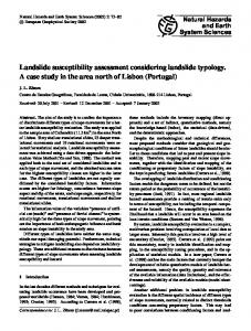
In this paper, we applied the widely used Bayesian bi-variate weights-of-evidence (WofE) susceptibility model to carry out two types of assessments. The former is focused on testing the susceptibility success and prediction skill using three different sampling strategies of the scarp area: (i) the centroid, (ii) points selected every 50 m, and (iii) the entire polygon. The latter is an analysis of the performance of the WofE susceptibility mapping when using different landslide sample sizes. In order to study the applicability and compare our analysis in different areas, we applied our assessments to two study areas, completely different in terms of size, geoenvironmental settings, and most importantly, different landslide types, namely debris flows and shallow landslides. The aim is to compare the performance of the WofE model in our two tests sites, to find which of the three landslide sampling strategies is the best suitable for each case study area, and to determine the minimum number of landslides needed in each area for sufficient susceptibility success and prediction results. 2. Case study areas The first area is the Fella River basin, with a total size of ~ 760 km2 (Fig. 1), located in the eastern Italian Alps (province of Udine, FriuliVenezia Giulia region). The area borders Austria and Slovenia and is part of an important corridor for international travel and logistics, winter tourism, and a gas-pipeline route. Land cover consists of predominately forested areas (75%), with ~10% bare surface and 8% grasslands, with the urban areas located along the valley bottoms and on alluvial fans (Malek et al., 2014). The geology is made up of Permian and Triassic rocks covered by Quaternary deposits. The Permian rocks consist of the Bellerophon unit with dolomite and black limestone, while the Triassic rocks are made of the Werfen Formation with calcareous-marls and the Serla Formation consisting of dolomite and dolomitic limestone (Calligaris et al., 2008). Quaternary deposits are found across the study area in the form of debris screes and glacial and alluvial deposits. Elevation ranges from 250 to 2750 m asl, with a mean slope value of 33°. The multiple systems of monoclines, bends, and faulting have caused extreme fracturing of bedrocks and outcropping of calcareous dolomitic sequences. This has led to the formation of very steep talus and scree slopes producing large amounts of debris stored within many secondary streams and debris flow channels flowing towards the Fella River. The latest major debris flow event occurred in August 2003, where ~1 million m3 of debris was triggered by an extreme rainfall event and deposited downslope at the bottom of the valleys. This event was also the cause of a major flood of the Fella River basin

(Tropeano et al., 2004). The area further regularly experienced shallow and deep-seated landslides (Pasuto et al., 2000) and flash flooding (Creutin and Borga, 2003; Borga et al., 2007, 2008). The second study area is the northern part of Buzau County (Romanian Carpathians) and has a total area of 3230 km2 (Fig. 1). Buzau County consists partly of hilly and mountainous (subCarpathians and Carpathians) areas, with the other half consisting of lower-lying plains (Sarata-Buzau plain). The high-altitude, northwestern half outlines two parallel regions with different morphological process patterns. The internal part corresponds to the Buzau Carpathians, a low- to mid-altitude mountainous sector built on Cretaceous and Paleogene flysch, with packs of generally cohesive sandstones alternating with schistose sandstones and clayey-marly schists. The Carpathians, reach a maximum elevation of 1700 m. The slopes, usually covered by relict landslide deposits, show inclinations of 15 to 45°. The external Buzau sub-Carpathians are a low to high sector of alternating rounded hills and large depressions. The area contains less cohesive and heterogeneous Mio-Pliocene molasse deposits, with a mix of marls, clays, sands, gravels, and large salt massifs and diapire folds, including small areas with loose schistose sandstones. The rounded hills extend from 250 to 900 m in altitude, while the dense river network is situated at 300–500 m. The slopes, intensely affected by active landslides, have inclinations ranging from 10 to 30°. Numerous relict or dormant landslide deposits, show high reactivation potential, with a number of active debris and rock slides featuring a high magnitude-low frequency pattern (Micu and Bălteanu, 2013). The sub-Carpathian slopes are more frequently affected by medium- and low-magnitude mudflows and shallow to medium-seated translational and rotational earth and debris slides (Micu and Bălteanu, 2013). 2.1. Landslide inventories and thematic data The debris flow inventory of the Fella River basin (Fig. 1) was produced through the analysis of historic archives and interpretation of aerial and satellite imagery between 1999 and 2011 by the Italian Landslide AVI and IFFI projects, the Geological Service of the Friuli–Venezia Giulia region (FVG) and landslide experts at University of Trieste. The inventory consists of 1046 debris flow scarp area polygons, excluding the accumulation zone. The Buzau County contains 1612 shallow landslide scarp areas (Fig. 1) mapped from image interpretation of aerial orthophotos between 2005 and 2008 and integrated with information obtained from the Romanian Emergency Situation Inspectorate (ISU) and field observations.

Fig. 1. Location of landslides and relief map of the two case study areas. On the left the Fella River basin (Friuli–Venezia Giulia region, Italy) and on the right Buzau County (Romania).

H.Y. Hussin et al. / Geomorphology 253 (2016) 508–523

The digital elevation model (DEM) of the Fella River basin was acquired from airborne laser scanning by the Civil Protection of the Friuli–Venezia Giulia region in 2003. The DEM has a pixel resolution of 20 m, which is the pixel dimension we used for all the causative factor maps and the susceptibility zonation. According to a previous study (Hussin et al., 2013), five causative landslide factor maps (lithology, land-cover, altitude, plan curvature, and slope) were used for the debris flow susceptibility zonation. The lithological map available at 1:150,000 scale was produced by the FVG Geological Service and originally contains more than 35 classes, which were reclassified in 8 classes. The land-cover map at 1:100,000 scale was developed by the CORINE land cover project and later updated by the MOLAND project. The map with more than 30 classes was generalized to 7 classes based on similarities in land cover types. The three factors derived from the DEM were classified into 10 quantile classes. The quantile classification has been applied in several landslide susceptibility studies (Castellanos Abella et al., 2008; Blahut et al., 2010; Martha et al., 2013) and is useful to proportionately distribute rank-ordered data to better study the influence of factors on landslide occurrence. The Buzau County DEM with a pixel resolution of 25 m was derived from the contour-lines of a 1:25,000 scale topographic map produced in 1984. The five landslide causative factor maps (altitude, internal relief (m/ha), slope, land cover, and soil) used for the shallow landslide susceptibility analysis were selected in previous studies (Hussin et al., 2013; Zumpano et al., 2013, 2014). The three DEM-derived factors were classified into 10 quantile classes. The land cover map at 1:5000 scale was derived from aerial photo interpretation and contains 9 classes. The soil map at 1:200,000 scale is classified in 11 classes and was derived from the Soil Maps of Romania updated from 1963 to 1994. The soil map was used instead of the geology owing to the nature of the shallow- to medium-seated landslides. Soil information was a better indicator of landslide initiation because it better represented the unstable shallow material properties, while the lithological map represented the bedrock. Preliminary tests were carried out using the lithological map, resulting in poor prediction of landslides, which indicated that the lithological data available was much less significant than the soil data (Zumpano et al., 2014). Table 1 summarizes the differences between the two case study areas. They are significantly different in terms of size, geology, morphology, and landslide types. Buzau County is more than four times larger than the Fella River area but has a landslide (centroid) point density half of the Fella River basin. The model pixel sizes are different due to the difference in the DEM resolution, but the pixel dimensions (20 and 25 m) can be considered similar and comparable for the purpose of the analysis.

511

Table 1 List of the thematic data and area statistics for the Fella River basin and Buzau County. Information Geoenvironmental factors DEM-derived factors Landslide type Study area size Landslide area Pixel size Total number of pixels Number of landslide pixels Number of landslides (centroid points) Landslide (centroid) point density per km2

Fella River basin

Buzau County

Lithology Land-cover Altitude Plan curvature Slope Debris flows 764.75 km2 7.25 km2 20 m 1,911,883 18,125 1046

Soil map Land-cover Altitude Internal relief Slope Shallow landslides 3230.57 km2 9.76 km2 25 m 5,168,940 15,551 1612

1.368

0.499

the importance of the presence of this class on the occurrence of landslides. The table also has the negative weight (W−), which evaluates the importance of the absence of the class on landslide occurrence and the contrast (W+ − W−). The contrast is considered a measure of the overall importance of a factor map class on the conditions causing landslide occurrence. One of the main advantages of the WofE approach is the capability of combining the subjective choice of the classified factors by the expert with the objective data-driven statistical analysis of the GIS. For details on the WofE methodology applied for landslide susceptibility the reader is referred to Lee et al. (2002). The calculation of weight tables for each factor and the subsequent susceptibility mapping was carried out using the weights-of-evidence Arc-SDM (spatial data modeller) (Sawatzky et al., 2009) geoprocessing tools in ArcGIS 10. In order to directly compare multiple WofE probability maps, the maps were standardized by reclassifying the probabilities using an area-based ranking (Chung and Fabbri, 2003; Lee, 2005; Pradhan, 2011; Sterlacchini et al., 2011; Akgun, 2012; Galve et al., 2014). We therefore classified the probability maps into 10 equal-area classes, with 10 classes being a compromise between very few classes with a lower descriptive power and the difficulty in interpreting too many classes. Success rate curves (SRCs) and prediction rate curves (PRCs) (Chung and Fabbri, 1999, 2003) were calculated to evaluate the model performance and the predictive skill of the susceptibility maps. The area under the curve (AUC), which is a value ranging between 0 and 1 or expressed as a percentage from 0 to 100%, was used as a final assessment of the SRCs and PRCs (Chung and Fabbri, 1999, 2003; Carrara et al., 2008; Blahut et al., 2010).

3. Methodology 3.2. Landslide sampling strategies and sizes 3.1. Weights-of-evidence (WofE) susceptibility model To prepare the landslide susceptibility maps, we applied the statistical weights-of-evidence (WofE) method in both study areas. The WofE technique was originally developed for quantitative mineral potential mapping to predict the location of possible gold deposits (BonhamCarter et al., 1989). However, it has been successfully applied in many landslide susceptibility assessments (van Westen, 1993; Lee et al., 2002; Süzen and Doyuran, 2004; Neuhäuser and Terhorst, 2007; Thiery et al., 2007; Blahut et al., 2010; Regmi et al., 2010; Ozdemir and Altural, 2013) and is based on the assumption that factors causing landslides in the past will determine the spatial occurrence of future landslide initiation in areas currently free of landslides. A probabilistic Bayesian approach is applied to determine the conditional probability between the presence/absence of each causative factor and the presence/absence of a landslide. For every factor map (e.g., land cover, lithology, etc.) a weighting table is produced that includes for each class (e.g., grassland, bare rock) the positive weight (W+), which indicates

The sampling strategies and sizes exploited to prepare susceptibility models in both test areas are summarized in Fig. 2. The vector-based representation of the landslide inventory determines which pixels are identified as landslide scarp areas. Once the landslide and nonlandslide pixels are determined, they can be selected to prepare the subsets to train the susceptibility model (training set) and to assess its predictive capability (prediction set). Two different sampling strategies were exploited. The first consisted of pixels corresponding to the scarp polygon centroid points. If the center of gravity of the polygon was located outside the scarp area, an ArcGIS operation was applied to force the centroid point to be located inside the polygon boundary. The second inventory consisted of pixels corresponding to points within the scarp polygon separated by a 50-m grid. The third contained all the pixels corresponding to the landslide scarp. The three inventories were randomly sampled into two subsets, with each subset containing 50% of the pixels. The first subset was used to train the susceptibility model to create the susceptibility map

512

H.Y. Hussin et al. / Geomorphology 253 (2016) 508–523

and produce the SRCs. The second subset was applied to test how well the model was able to predict landslides using the PRCs. The sensitivity of the WofE susceptibility model to landslide sample size was tested using the centroid sampling method. As with the sampling strategy test, all the nonlandslide (absence) pixels were considered in the sensitivity analysis. Different landslide (presence) pixel samples were randomly sampled from the centroid inventory of each study area. The 1046 debris flow scarp centroids of the Fella River basin were randomly sampled into the following sizes: 31, 52, 104, 209, 523, 836, and 941 and correspond respectively to 3, 5, 10, 20, 50, 80, and 90% of the inventory. The Buzau County 1612 shallow landslide centroids were randomly sampled into sample sizes of 80, 161, 322, 806, 1290, 1451, which also corresponded respectively to 5, 10, 20, 50, 80, and 90% of all shallow landslide centroids. These samples were used as training subsets but also as prediction subsets. For example, when 10% was randomly sampled for training, the remaining 90% was considered as a prediction subset. However, the same 90% was also used to train the model, while the same 10% was used for model prediction. Therefore, every sample size between 10 and 90% had one chance to be the training and prediction subset. 4. Results Fig. 3 shows the WofE susceptibility model contrast values of the factor map classes for the different landslide sampling strategies. Bare rock areas in both case studies are a significant source of landslide scarps in terms of land cover. The lithology most contributing to debris flow sources in the Fella River Basin is dolomite and limestone, while the soil types in Buzau County having the most influence on shallow landslide scarps are the Aquisalids and Erodisols. Fig. 3 also indicates that in the Fella area the presence of debris flow sources is generally more significant as the altitude, plan curvature, and slope increase. In Buzau County, shallow landslides are mainly focused in areas in the middle altitude and slope ranges.

The WofE contrast values related to the sample size sensitivity test are shown in Figs. 4 and 5 for the Fella River basin and Buzau County, respectively. The overall trend in contrast values between the factor classes is similar to the ones in Fig. 3. However, for each class within a factor map, different trends were found when increasing the landslide training sample size for the susceptibility modeling. Fig. 4 shows that in the mud- and sandstone class of the lithology map, there is an increase in the negative contrast as the sample size increases, indicating that the more landslides are used to train the model, the less that mud- and sandstone has an effect on landslide occurrence. In some cases there is not a clear trend. Fig. 5 also shows a negative contrast of slope class 35–38° when using 52 scarp centroid pixels. This same class shifts to a positive contrast after using 104 landslide pixels to train the model. An opposite trend can be seen in certain altitude classes, where an increase in the sample size shifts the contrasts from positive to negative or lower values (Figs. 4 and 5). This is possibly caused by a shift in distribution of landslide pixels to different altitude classes as the surface area representing the scarp polygon increases. The largest shifts in contrast values for the Fella River basin (Fig. 4) are found in the forest class of the land cover map, the 1037–1160 m class of the altitude map, and the 31–35° class of the slope map. For Buzau County (Fig. 5) the largest shifts are found in the altitude classes and the classes of the internal relief factor map. The susceptibility maps that were produced using landslide centroid pixels and classified into 10 equal area classes are shown in Fig. 6. For the Fella River basin, the AUC values for the SRC and PRC were 82.53% and 81.26%, respectively. The Buzau County susceptibility map produced AUC values of 79.77% for the SRC and 79.49% for the PRC. The debris flow source susceptibility in the Fella River basin is higher in areas with high slope angles and where bare rocks are most persistent. Whereas the shallow landslide susceptibility in Buzau County is higher in the middle altitude and slope angles and follows more or less the boundary between the Carpathians and lower sub-Carpathians. These results also correspond well with the contrast values previously shown in Fig. 5.

Fig. 2. Flow chart showing the method used to prepare training and prediction subsets for the WofE susceptibility model.

H.Y. Hussin et al. / Geomorphology 253 (2016) 508–523

513

Fig. 3. Weights-of-evidence contrast values (W+ − W−) of each factor map for the different sampling strategies in (A) the Fella River basin and in (B) the Buzau County. The acronyms of the soil classes are taken from the Romanian System of Soil Taxonomy (RSST-2000, in Romanian) and translated according to the USDA Soil Taxonomy, 1999 (Florea and Munteanu, 2000): AA = alluvial protosoil; AP = water; BD = brown argilloilluvial soil; BM = brown eu-mesobasic soil; BO = brown acid soil; BP = brown luvic soil (podzolite); BR = brown–red soil; CC = cambic chernozem; CI = argilloilluvial chernozem; CN = gray soil; CZ = chernozem; ER = erodisoil; LC = hydromorphic soil; LS = litosoil; NF = black clinohydromorphic soil; NO = black acid soil; PB = brown iron-illuvial soil (podzol); PD = podzol; PR = pseudo rendzine; PS = psamosoils; RP = brown-reddish luvic soils; RS = regosol; RZ = rendzina; SA = alluvial soil; SC = aquisalids; SN = solonetzs; SP = albic-luvic soil (argilloilluval podzol).

Fig. 7 shows sections of the susceptibility maps for each of the three tested landslide sampling strategies. In both areas, there is a noticeable increase in medium to high susceptible areas when comparing the centroid method with the polygon strategy. The centroid method also

seems to show different boundary conditions in the low to medium susceptibility classes compared to the other methods. In Buzau County, there is a slightly stronger shift in susceptibility to higher classes going from centroid to 50-m points. Overall, the Fella River basin has more

514

H.Y. Hussin et al. / Geomorphology 253 (2016) 508–523

Fig. 4. Weights-of-evidence contrast values (W+ − W−) for each factor map applied in the susceptibility assessments using the different sample sizes in the Fella River basin.

changes in susceptibility mapping with the different strategies than in Buzau County. The WofE model SRCs and PRCs using different landslide sampling strategies are presented in Fig. 8, which also includes the AUC values in percentages. For the Fella River basin, AUC values for SRCs and PRCs show a slight increasing trend in success and prediction as the number of pixels representing the landslide scarp increases. The centroid method gives an AUC SRC of 82.53%, while modeling with the 50-m grid points and the scarp polygons give AUC values of 83.81% and 84.64%, respectively. The increase in success rate is less evident in Buzau County, with the highest AUC SRC value given by the 50-m grid points. This indicates that using Buzau County scarp polygons should be avoided due to possible redundant information from oversampling of too many points, causing fitting problems. This coincides with a similar finding in a previous study conducted by Poli and Sterlacchini (2007). However, the prediction rate in the Buzau County is highest when modeling with the entire polygon, with an AUC PRC value of 80.66%. There is little difference between the AUC SRCs and AUC PRCs, with overall prediction rates being only slightly higher. Fig. 9 shows a section of the susceptibility maps produced with sample size testing. By using 52 (5%) landslides to train the model in the Fella River basin, some areas are highly underestimated, with generalizations occurring at low to medium classes. Susceptibility maps made with 52 (5%) to 104 (10%) landslides also show grainy pixelated maps with boundaries between susceptibility classes being less continuous. It seems that when the landslide pixel sample is too small, the likelihood of random sampling from a factor class that contains more landslide pixels increases, causing a bias in the sample and possible conditional dependence problems. The abrupt shifts in the susceptibility classes

that most likely follow the lithology also correspond to the very high contrast found in the dolomite and limestone areas when using 5% of the centroid pixel inventory (Fig. 4). Models using 50 to 90% perform spatially better, predicting more landslide areas and having smoother transitions from lower to higher susceptibility classes. The Buzau County susceptibility maps also show variation in medium to high susceptibility classes when increasing the number of landslides used in the WofE modeling. Some of the low to medium susceptibility classes produced with 5 to 20% of the landslides in Buzau County change to higher classes when using 90% of the centroid pixels. The SRCs and PRCs related to the landslide sample size sensitivity analysis are shown in Fig. 10 for both study areas. The curves for the Fella River Basin indicate that as the number of landslides used to train the WofE model increases, the performance and prediction rates also increase. The trend in success and prediction rates continues to increase up to 83.87% and 82.79%, respectively, when using a maximum of 941 landslides for model training to predict the remaining 104 landslides. However, the strongest increase occurs when at least 104 (while 941 are used as a prediction subset) landslides are used to train the model, producing an AUC SRC value of 81.45% and an AUC PRC value of 81.73%. This indicates that when using the WofE model in the Fella River basin, 104 landslides are enough to accurately predict the occurrence of the rest of the 941 landslides used as a prediction subset. In Buzau County, the best success rates are obtained using at least 322 landslides to train the model, while the best prediction is made using a 50/50% ratio between the number of training and prediction landslides. Buzau County does not indicate a clear increasing trend in success and prediction when compared to the Fella River basin.

H.Y. Hussin et al. / Geomorphology 253 (2016) 508–523

515

Fig. 5. Weights-of-evidence contrast values (W+ − W−) for each factor map applied in the susceptibility assessments using the different sample sizes in Buzau County.

One of the limitations of this work is the use of only one random sample of the landslide centroids used to train the WofE model for each sample size. Therefore, in order to study the effect of the sampling procedure, we took 10 random samples for each sample size in the Fella River basin. The results of the success and prediction rates for the 10 random samples of all seven sample sizes is shown in Table 2. The mean AUC values show an increase as the number of landslides are

increased to train the model. There is also a significant decrease in the standard deviation of the 10 random samples when using 200 or more landslides, decreasing the error substantially after using 20% or more of the inventory for training the model. The AUC prediction rates show a similar increase as the success rates. The overall trend in AUC values with 10 random samples is still similar to using a single random sample for each landslide sample size.

Fig. 6. Best performing susceptibility maps modeled with landslide centroid pixels for (left) the Fella River basin and (right) the Buzau County case study areas.

516

H.Y. Hussin et al. / Geomorphology 253 (2016) 508–523

Fig. 11 graphically shows the AUC values related to the SRCs and PRCs in Fig. 10 for Buzau County and the average values in Table 2 for the Fella River basin. As the number of landslides used to train the model in the Fella River basin increases up to 100, the AUC value rapidly increases from 61 to 82%. After using 100 to 200 landslides, the increase in AUC is very gradual with a plateau effect visible in the performance and prediction rates. This effect is not visible in the AUC success rates in Buzau County, with only a 5% increase in AUC prediction rate from 75 to 80% when increasing the training sample from 100 to 800 landslides. However, in Buzau County after training the model with more than 1400 landslides, a drop in the prediction rate occurs from 79 to 76% when trying to validate the remaining 160 landslides. 5. Discussion One of the limitations of this work was the problem of accuracy and quality of the input data consisting of the landslide inventories and the causative factor maps. Mapping errors are very common when mapping many landsides in an area, especially when the landslides in one area have been mapped by different people or institutions. We have attempted to reduce this error by removing landslides that we considered incorrectly mapped, but the errors cannot be completely avoided. Another important point is the scale of the thematic maps (e.g., geological, soil, and land cover) in comparison with the grid-cell resolution selected for susceptibility mapping. Using small-scale maps (e.g., 1:100,000 to 2:200,000) causes higher geographic inaccuracies, where a few millimeters on the factor maps can translate into errors of several grid cells of 20 or 25 m in the GIS used in this study. This is especially the case at the boundaries between different thematic units and when using maps of different scales for the causative factors. The effect of these errors and inaccuracies on susceptibility mapping should be investigated in upcoming studies. The weights assigned to each class within a causative factor map in the WofE model is determined by the number of landslide pixels counted in each class and the difference in the number of pixels between the classes. The tests carried out using different sampling strategies basically increases the number of pixels that are assigned to each landslide for susceptibility modeling, thereby increasing the landslide area in a causative factor class. The results in Fig. 8 show in the Fella River basin that there is a slight increase in success and prediction rates associated with the increase in pixels representing the landslide scarp polygons. This is in agreement with findings in previous studies (Poli and Sterlacchini, 2007; Thiery et al., 2007; Yilmaz, 2010; Regmi et al., 2013). However, this increase is not evident in Buzau County, where no change is found in model performance between the use of centroids and scarp polygons (Fig. 8). Despite a significant increase in the number of landslide pixels to represent the entire landslide scarp polygon, there is little difference in the overall model performance and prediction between the sampling strategies. In order to understand these results, Table 3 is required, which shows the percentage increase in number of landslide pixels as the sampling strategy changes for two causative factors in both case study areas. These are land cover and lithology for the Fella River basin and land cover and soil for Buzau County. The percentage increase for most factor classes is very similar, particularly in the classes that have many pixels. This similarity will cause very little change in the weights of the individual factor map classes when increasing the pixels for different sampling strategies. This is most likely caused by the scarp polygons having similar sizes throughout the study area. If the landslide scarp polygons are of similar size, the relative increase in the number of pixels to represent each polygon will be similar for all the scarps. Changing the representation of a single scarp in a certain factor class from 1 pixel to, for example,

10 pixels, will allocate a similar increase in pixels to a scarp polygon located in a different class. The chances of this problem occurring can be high because landslide susceptibility assessments are mainly carried out using a single landslide type, without mixing landslides of different types and therefore different sizes. The landslide sizes, including the sizes of the scarps should be assessed statistically in more detail in further studies in order to further analyze the limitation of using single centroid points/pixels in susceptibility modeling. Table 3 also gives us an indication why our model performs slightly better in the Fella River Basin when we change the sampling strategy compared to Buzau County. The average percentage increase in the number of pixels in each factor class from the centroid strategy to 50-m points in the Fella River basin is 414%, while the average increase from 50-m points to the polygon strategy (all pixels) is 527%. However, in Buzau County, the percentage increases for the same tests are 102% and 190%, respectively. In other words, the landslide area in Buzau County increases 2 to 3 times more when using polygons instead of centroids, while in the Fella River basin the area increases 5 to 6 times. This much larger increase in landslide size in the Fella River basin will still show some significance in success and prediction rates of the susceptibility model compared to that of Buzau County. As the landslide sample size increases with the use of different landslide sampling strategies, a relationship is expected between landslide sampling strategy and landslide sample size in terms of the number of pixels that represent the inventory and the training and prediction subsets. It is highly recommended to assess this relationship in more detail in future studies. The sampling strategy tests show similarities between the area under the SRCs and PRCs (AUC). When the WofE model has similar performance values as the prediction values, this indicates that the training and prediction subsets fit the model equally well. This is most likely because of the pixels being sampled from the same landslide polygon causing both subsets to perform similarly. Training and prediction pixels represent more or less the same causative factor combinations that will produce similar success and prediction rate curves of the susceptibility model. This indicates that it is recommended to randomly sample entire polygons into separate success and prediction subsets so that pixels from a single polygon are not separated from each other and thereby decrease the possibility of oversampling or overfitting. This problem has been most recently described by San (2014) where he indicates that ‘polygon-based random sampling is recommended for collecting the training and testing data’ and, therefore, is preferred over pixel-based random sampling as used in this paper. However, we have avoided this problem when using only the centroids in the sample size sensitivity tests. Because one of the goals of this study was to give some recommendations on the percentage of landslides (from the total inventory) needed to train the WofE model, it is important to compare our work with previous research. Most studies consider taking 50% of the inventory to train the WofE model (e.g., Blahut et al., 2010; Regmi et al., 2013), while others use higher values ranging from 65 to more than 80% of the inventory (e.g., Neuhäuser and Terhorst, 2007; Pradhan et al., 2010; Ozdemir and Altural, 2013). Rarely has the effect of training the model with b50% been studied. In our work, the sample size testing to train the WofE model shows that a minimum number of landslides are needed to produce sufficient model performance and prediction results. Fig. 11 indicates that in the Fella River Basin, there is a minimum of 104 to 209 (10 to 20% of the inventory) out of a total of 1046 landslide centroids required to produce SRCs and PRCs with AUC values above 80%. Using more than 104 centroid pixels slightly increases the AUC for performance and prediction but starts to show a plateau with little change in the overall values after using 200 or more landslide centroids.

Fig. 7. Sections of the susceptibility maps modeled using the three different types of landslide sampling strategies. From top to bottom: susceptibility modeled with scarp centroids, 50-m grid points and the landslide polygons.

H.Y. Hussin et al. / Geomorphology 253 (2016) 508–523

517

518

H.Y. Hussin et al. / Geomorphology 253 (2016) 508–523

Fig. 8. Success (SRC) and prediction (PRC) rate curves of the WofE susceptibility models using the three different landslide polygon sampling strategies.

This plateau in performance corresponds well with recent previous studies (Hjort and Marmion, 2008; Guns and Vanacker, 2012; Heckmann et al., 2014; Petschko et al., 2014). The Buzau County AUC SRCs do not show a clear trend as in the Fella River basin, with a peak AUC SRC of 80.18% found when using 322 from a total of 1612 landslide centroids (Fig. 11). However, the AUC PRCs in the Buzau County do indicate that a minimum of 161 landslides are needed for an acceptable prediction rate of 78.84%, while more training landslides produce a similar plateau as seen in the Fella River basin. The Buzau County susceptibility map trained with 80 landslides has difficulty predicting the remaining 1531 landslides. As expected, the AUC values of the SRCs in both areas are generally slightly higher than the AUC values of the PRCs. It is interesting to note that in Buzau County, when training the model with 1531 landslides to predict the remaining 80, the prediction rate decreased from 79.35 to 76.93%. A possible reason for this drop could be that the much larger Buzau County has an uneven distribution of mapped landslides, where the northern part of the county is less represented in the mapping process. Furthermore, there are also possible mapping inaccuracies and incompleteness in the landslide inventory in this area. Another limitation in this work was the use of only one random sample for each landslide sample size tested. For this reason, extra random samples were conducted related to Table 2, which gave us some indication of error estimates when more than one sample was taken. These were, however, only 10 random samples. More sample runs are required to properly study the effect of chance and error of the random sampling procedure. The Fella River basin and Buzau County success and prediction rates could be improved if many random samples would have been conducted. We therefore

recommend to carry out many random samples for both areas in the future, possibly up to 50, 100, or even 1000 model runs (Brenning, 2005; Beguería, 2006; Van Den Eeckhaut et al., 2010; Heckmann et al., 2014) to get a more accurate view on the effects of sampling different landslide sample sizes on the success and prediction rate of the susceptibility model. By conducting the sample size tests, we have analyzed the performance of the WofE model to changes in the ratio between landslide training and prediction pixels. The analysis has shown that for two areas with completely different sizes (~765 and ~3231 km2) and landslide types (debris flows vs. shallow landslides), a training to prediction subset ratio of 1:9 (10%:90%) produces sufficient model performance and prediction, with both areas containing more than 1000 landslide centroid grid points (pixels). The use of 10% of the landslide inventory is equal to 161 landslide pixels in Buzau County and 104 pixels in the Fella River basin. This corresponds with a landslide to nonlandslide pixel ratio of 1:32,105 and 1:18,208, respectively. The WofE landslide susceptibility model has performed slightly better with the debris flows in the Fella River basin than with the shallow landslides of Buzau County. As the landslide pixel sampling strategy increased from a single centroid to the entire polygon, so did the success and prediction of the debris flow source areas slightly increase, with most debris flow sources also significantly increasing in the number of pixels. In Buzau County, the shallow landslides did not show this significant increase in pixels representing the scarp areas. This could indicate that the scarp areas of the shallow landslides are too small for the given mapping unit of 25 m. Furthermore, because of the small scale and the difference in scales of the factor maps, the quality and accuracy of susceptibility is negatively affected. Thus, the scale and resolution of the

H.Y. Hussin et al. / Geomorphology 253 (2016) 508–523

519

mapping unit are a very important issue in landslide susceptibility mapping and prediction (Catani et al., 2013). Other mapping unit sizes should also be assessed, considering the factor maps with the smallest scales. The maximum obtained success and prediction rates using different landslide centroid sample sizes were higher for the Fella River basin than Buzau County. The increase in the model performance when increasing the number of landslides used for model training were much more significant for the debris flows than the shallow landslides. However, in the future, more susceptibility models should be run in Buzau County for smaller sample sizes (b100 landslides) to better study the significance of possible sample size thresholds in larger areas that have been known to occur in previous studies (Hjort and Marmion, 2008; Heckmann et al., 2014). Overall, the WofE model in Buzau County does not perform as well as in the Fella River basin. One of the main reasons for this is that the inventory of the shallow landslides was mainly mapped for the southern part, with the northern part not well represented (Fig. 1). This is because the Romanian Emergency Situation Inspectorate (ISU) were more interested in the higher populated areas in the south. The shallow landslides in the south affected more roads and farm land, with the area considered a higher risk zone. After taking a closer look and conducting further discussions on the Romanian landslide data, more mapping errors were found, also indicating that the experts did not have much experience in mapping landslides. Even with similarities in modeled success and prediction rates found in the landslide sampling strategies, there are still some visible differences in the classified susceptibility maps. This indicates that the spatial variation between the similar performing susceptibility maps can be different. A susceptibility map trained with 100 landslides can give similar performance rates (AUC values) as a map made using 500 landslides but still looks very different after classifying the maps using the same method. A spatial agreement analysis (Sterlacchini et al., 2011) can be carried out in future studies in order to determine the best susceptibility classification by taking into consideration all maps that show similar performance and prediction rates but different predicted patterns. This is important in order to communicate to decision makers, land use planners, and responsible authorities the right maps to assess landslide hazard and risk. 6. Conclusions

Fig. 9. Sections of the landslide susceptibility maps in both study areas modeled with different sample sizes. From top to bottom: sample size percentages used were 5, 10, 20, 50, 80, and 90%. Black polygons indicate the original scarp area, with the black points indicating the centroids.

The weights-of-evidence landslide susceptibility model was applied in the Italian Alps using debris flow scarps and in the Romanian Carpathians using shallow landslides. Three different landslide sampling strategies were tested in the susceptibility analysis: (i) the centroid scarp point, (ii) points located every 50 m within the scarp, and (iii) the entire scarp polygon. The shallow landslides in Buzau County (Romanian Carpathians) gave better success rates when sampled using the 50-m grid point method, while the scarp polygon method was better in predicting the shallow landslides. The susceptibility model assessing the debris flow scarps in the Fella River basin (Italian Alps) had better success and prediction rates when using the entire scarp polygon compared to the other strategies. Overall, the model performed better using debris flows scarps than the shallow landslides. The number of landslides was similar for both case studies; however, the Romanian site was four times larger with some areas being underrepresented in terms of mapping and quality of the data. The effect of the landslide training sample size on the susceptibility performance rates was assessed. In the Fella River basin, a training subset threshold of 104 debris flow scarps was sufficient to predict the remaining 941 scarps, giving success and prediction rates (AUC values) above 81%. Buzau County required a training subset of at least 161 shallow landslide scarps to predict the remaining 1451 scarps with success and prediction rates above 79%. Both case study areas needed at least 10 to 20% of the landslide inventory to train the model and produce adequate success and prediction rates. When training subsets were used

520

H.Y. Hussin et al. / Geomorphology 253 (2016) 508–523

Fig. 10. SRCs, PRCs, and AUC values for susceptibility maps modeled with different landslide sample sizes.

that contained landslide numbers below these thresholds, model performance was significantly lower. However, using more landslides above the thresholds caused success and prediction rates to plateau

with only a slight increase in model performance. This threshold was more obvious with the Italian debris flows than the Romanian shallow landslides.

Table 2 Weights-of-evidence susceptibility success and prediction rates for 10 random samples of each landslide sampling size in the Fella River basin study area; the table has information on the statistics of the success and prediction rates, including the mean value of the 10 models for each sampling size and the standard deviation. Number of landslides used for model training

% of all landslides

Area under the success rate curve (SRC) (%)

Statistics for the 10 model runs

1

2

3

4

5

6

7

8

9

10

Mean

Std

31 52 104 209 523 836 941

3 5 10 20 50 80 90

60.4 75.2 81.5 82.1 82.5 83.8 83.9

59.5 75.5 79.9 81.9 83.2 83.2 84.8

61.8 75.9 79.2 82.0 82.0 83.3 83.5

59.3 72.3 77.8 82.6 82.5 83.9 83.9

59.1 75.3 82.3 82.3 83.0 83.8 84.2

59.8 74.7 80.6 81.8 82.4 83.7 83.0

59.8 74.4 78.3 82.4 82.2 82.9 84.6

61.4 73.1 80.5 81.8 83.0 82.6 83.0

59.1 76.6 80.9 82.7 82.1 83.9 84.4

60.7 73.5 79.0 82.9 83.1 83.3 84.7

60.1 74.7 80.0 82.3 82.6 83.4 84.0

0.96 1.34 1.43 0.39 0.44 0.45 0.66

Number of landslides used for model prediction

% of all landslides

Area under the prediction rate curve (PRC) (%)

1015 994 941 836 523 209 104

97 95 90 80 50 20 10

Statistics for the 10 model runs

1

2

3

4

5

6

7

8

9

10

Mean

Std

61.3 74.0 81.7 81.1 81.3 82.4 82.8

59.1 71.2 82.0 81.2 80.8 82.6 83.8

59.9 74.0 81.2 81.1 81.9 82.0 83.4

62.3 70.7 81.8 81.1 81.8 81.6 83.9

60.8 75.0 81.1 81.4 81.0 82.4 83.4

59.3 76.0 80.7 81.6 81.5 82.8 83.7

60.5 70.7 81.9 80.7 80.9 82.3 83.2

60.5 75.9 80.5 81.8 81.9 82.0 83.7

60.3 70.3 80.1 81.5 81.2 82.4 82.9

59.1 74.6 80.7 80.4 81.8 82.4 82.9

60.3 73.2 81.2 81.2 81.4 82.3 83.4

1.02 2.27 0.66 0.42 0.43 0.34 0.41

H.Y. Hussin et al. / Geomorphology 253 (2016) 508–523

521

Fig. 11. The AUC values of the success rate (SRCs) and prediction rate (PRCs) curves for susceptibility models trained with different number of landslides from the available inventories. The red curves indicate the model success rates for different landslide training sizes, and the blue curves indicate the model prediction rates using different landslide prediction sample sizes.

Table 3 Number of landslide pixels located within the geoenvironmental factor map classes; the factors are land cover and lithology for the Fella River basin and land cover and soil for Buzau County (the last two columns on the right indicate the percentage increase in the number of pixels when changing the strategy from centroid to 50-m grid points and from 50-m grid points to using the entire scarp polygon considering all pixels within the polygon, respectively). Fella River basin Land cover

Centroid pixels

50 m grid point pixels

All scarp pixels

Percent increase Centroid → 50 m

Percent increase 50 m → all scarp pixels

Human infrastructure Agriculture Flood plain Woodland Grassland Forest Bare rock

0 0 2 44 70 157 80

0 0 3 148 365 729 1485

0 0 17 922 2279 4535 9199

– – 50% 236% 421% 364% 494%

– – 467% 523% 524% 522% 519%

Lithology

Centroid pixels

50 m grid point pixels

All scarp pixels

Alluvial deposits Intrusive rocks Mud- and sandstones Conglomerates Marls Debris and scree deposits Dolomitic marls Dolomite and dolomitic limestone

0 0 1 4 11 23 45 439

10 6 10 9 49 147 327 2172

53 30 56 77 318 933 2149 13,336

Percent increase Centroid → 50 m – – 900% 225% 345% 539% 627% 395%

Percent increase 50 m → all scarp pixels 430% 400% 560% 756% 549% 534% 557% 514%

Buzau County Land cover

Centroid pixels

50 m grid point pixels

All scarp pixels

Percent increase Centroid → 50 m

Percent increase 50 m → all scarp pixels

Vineyards Bushes Roads Orchards Houses/households Wetlands and waters Degraded land and bare rocks Forest Pasture and hayfields

0 1 7 12 18 24 36 206 497

0 7 7 13 26 32 104 330 713

1 35 21 36 40 75 331 1011 1988

– 600% 0% 8% 44% 33% 189% 60% 43%

– 400% 200% 176% 54% 134% 218% 206% 179%

Soil

Centroid pixels

50 m grid point pixels

All scarp pixels

AP SN/BR/RP PD/SP BD/CI SC SA/AA CN/NF/LC BP/PB BO/CC/CZ/NO BM/RS/LS/PS PR/ER/RZ

0 3 4 6 7 23 41 80 112 246 279

0 3 4 6 10 41 68 142 187 361 413

0 7 13 16 30 85 240 408 628 1013 1106

Percent increase Centroid → 50 m – 0% 0% 0% 43% 78% 66% 78% 67% 47% 48%

Percent increase 50 m → all scarp pixels – 133% 225% 167% 200% 107% 253% 187% 236% 181% 168%

522

H.Y. Hussin et al. / Geomorphology 253 (2016) 508–523

The comparison of the classified susceptibility maps produced using different sampling strategies and sample sizes indicated that there are significant differences in the lower to medium susceptibility classes despite having similar success and prediction rate values. It is therefore recommended in the future to combine the maps in order to assess where they spatially agree and how they can be used for decision makers. Acknowledgments This study is part of an ongoing landslide quantitative risk assessment (QRA) carried out within the EC FP-7 funded CHANGES network (Grant Agreement No. 263953). We thank Dr. Simone Frigerio, Dr. Alessandro Pasuto, Dr. Gianluca Marcato, and Dr. Chiara Calligaris for their efforts in data collection and sharing and for their valuable discussions and insights on the study areas. Many thanks go to the anonymous reviewers for their detailed comments and suggests on improving this paper. Finally, we would like to thank the editor, Dr. Richard Marston for the detailed editing and corrections made to this paper. References Akgun, A., 2012. A comparison of landslide susceptibility maps produced by logistic regression, multi-criteria decision, and likelihood ratio methods: a case study at İzmir, Turkey. Landslides 9 (1), 93–106. Aleotti, P., Chowdhury, R., 1999. Landslide hazard assessment: summary review and new perspectives. Bull. Eng. Geol. Environ. 58 (1), 21–44. Atkinson, P.M., Massari, R., 1998. Generalised linear modelling of susceptibility to landsliding in the Central Apennines, Italy. Comput. Geosci. 24 (4), 373–385. Ayalew, L., Yamagishi, H., 2005. The application of GIS-based logistic regression for landslide susceptibility mapping in the Kakuda–Yahiko Mountains, Central Japan. Geomorphology 65 (1–2), 15–31. Beguería, S., 2006. Validation and evaluation of predictive models in hazard assessment and risk management. Nat. Hazards 37 (3), 315–329. Blahut, J., van Westen, C.J., Sterlacchini, S., 2010. Analysis of landslide inventories for accurate prediction of debris-flow source areas. Geomorphology 119 (1–2), 36–51. Bonham-Carter, G.F., Agterberg, F.P., Wright, D.F., 1989. Weights of evidence modelling: a new approach to mapping mineral potential. In: Agterberg, D.F., Bonham-Carter, G.F. (Eds.), Statistical Applications in Earth Sciences. Geological Survey of Canada, Ottowa. Borga, M., Boscolo, P., Zanon, F., Sangati, M., 2007. Hydrometeorological analysis of the August 29, 2003 flash flood in the eastern Italian Alps. J. Hydrometeorol. 8, 1049–1067. Borga, M., Gaume, E., Creutin, J.D., Marchi, L., 2008. Surveying flash floods: gauging the ungauged extremes. Hydrol. Process. 22, 3883–3885. Brenning, A., 2005. Spatial prediction models for landslide hazards: review, comparison and evaluation. Nat. Hazards Earth Syst. Sci. 5 (6), 853–862. Brenning, A., 2009. Benchmarking classifiers to optimally integrate terrain analysis and multispectral remote sensing in automatic rock glacier detection. Remote Sens. Environ. 113 (1), 239–247. Calligaris, C., Boniello, M.A., Zini, L., 2008. Debris flow modelling in Julian Alps using FLO2D. In: De Wrachien, D., Brebbia, C.A., Lenzi, M.A. (Eds.), Monitoring, Simulation. Prevention and Remediation of Dense and Debris Flows II. Witpress, Southhampton, UK, pp. 81–88. Carrara, A., 1983. Multivariate models for landslide hazard evaluation. J. Int. Assoc. Math. Geol. 15 (3), 403–426. Carrara, A., Cardinali, M., Guzzetti, F., Reichenbach, P., 1995. Gis technology in mapping landslide hazard. In: Carrara, A., Guzzetti, F. (Eds.), Geographical Information Systems in Assessing Natural Hazards. Advances in Natural and Technological Hazards Research. Springer, Netherlands, pp. 135–175. Carrara, A., Crosta, G., Frattini, P., 2008. Comparing models of debris-flow susceptibility in the alpine environment. Geomorphology 94 (3–4), 353–378. Castellanos Abella, E.A., de Jong, S.M., van Westen, C.J., van Asch, T.W.J., 2008. Multi-scale Landslide Risk Assessment in Cuba (ITC PhD Dissertation 154) ITC, Enschede, University of Utrecht, Utrecht. Catani, F., Lagomarsino, D., Segoni, S., Tofani, V., 2013. Landslide susceptibility estimation by random forests technique: sensitivity and scaling issues. Nat. Hazards Earth Syst. Sci. 13 (11), 2815–2831. Chung, C.-J., Fabbri, A.G., 1999. Probabilistic prediction models for landslide hazard mapping. In: Buccianti, A., Nardi, G., Potenza, R. (Eds.), Proceedings of International Association for Mathematical Geology 1998 Annual Meeting (IAMG’98). Ischia, Italy, pp. 203–211 (October 1998). Chung, C.-J., Fabbri, A.G., 2003. Validation of spatial prediction models for landslide hazard mapping. Nat. Hazards 30 (3), 451–472. Chung, C.-J., Fabbri, A.G., 2005. Systematic Procedures of Landslide Hazard Mapping for Risk Assessment Using Spatial Prediction Models, Landslide Hazard and Risk. John Wiley & Sons, Ltd, pp. 139–174. Clerici, A., Perego, S., Tellini, C., Vescovi, P., 2006. A GIS-based automated procedure for landslide susceptibility mapping by the conditional analysis method: the Baganza valley case study (Italian Northern Apennines). Environ. Geol. 50 (7), 941–961.

Corominas, J., Westen, C., Frattini, P., Cascini, L., Malet, J.P., Fotopoulou, S., Catani, F., Eeckhaut, M., Mavrouli, O., Agliardi, F., Pitilakis, K., Winter, M.G., Pastor, M., Ferlisi, S., Tofani, V., Hervás, J., Smith, J.T., 2013. Recommendations for the quantitative analysis of landslide risk. Bull. Eng. Geol. Environ. 73 (2), 1–55. Creutin, J.D., Borga, M., 2003. Radar hydrology modifies the monitoring of flash flood hazard. Hydrol. Process. 17 (7), 1453–1456. Crozier, M.J., Glade, T., 2005. Landslide Hazard and Risk: Issues, Concepts and Approach, Landslide Hazard and Risk. John Wiley & Sons, Ltd, pp. 1–40. Dai, F.C., Lee, C.F., Ngai, Y.Y., 2002. Landslide risk assessment and management: an overview. Eng. Geol. 64 (1), 65–87. Demir, G., Aytekin, M., Akgün, A., İkizler, S., Tatar, O., 2013. A comparison of landslide susceptibility mapping of the eastern part of the North Anatolian Fault Zone (Turkey) by likelihood-frequency ratio and analytic hierarchy process methods. Nat. Hazards 65 (3), 1481–1506. Donati, L., Turrini, M.C., 2002. An objective method to rank the importance of the factors predisposing to landslides with the GIS methodology: application to an area of the Apennines (Valnerina; Perugia, Italy). Eng. Geol. 63 (3–4), 277–289. Felicísimo, Á., Cuartero, A., Remondo, J., Quirós, E., 2013. Mapping landslide susceptibility with logistic regression, multiple adaptive regression splines, classification and regression trees, and maximum entropy methods: a comparative study. Landslides 10 (2), 175–189. Fell, R., Corominas, J., Bonnard, C., Cascini, L., Leroi, E., Savage, W.Z., 2008. Guidelines for landslide susceptibility, hazard and risk zoning for land-use planning. Eng. Geol. 102 (3–4), 99–111. Florea, N., Munteanu, I., 2000. Sistemu Roman de Taxonomie a Solurilor (Romanian System of Soil Taxonomy). Univ. "Al. I. Cuza", lasi (107 pp.). Galli, M., Ardizzone, F., Cardinali, M., Guzzetti, F., Reichenbach, P., 2008. Comparing landslide inventory maps. Geomorphology 94 (3–4), 268–289. Galve, J., Cevasco, A., Brandolini, P., Soldati, M., 2014. Assessment of shallow landslide risk mitigation measures based on land use planning through probabilistic modelling. Landslides 12 (1), 1–14. Glade, T., Crozier, M.J., 2005. A Review of Scale Dependency ien Landslide Hazard and Risk Analysis, Landslide Hazard and Risk. John Wiley & Sons, Ltd, pp. 75–138. Gorum, T., Fan, X., van Westen, C.J., Huang, R.Q., Xu, Q., Tang, C., Wang, G., 2011. Distribution pattern of earthquake-induced landslides triggered by the 12 May 2008 Wenchuan earthquake. Geomorphology 133 (3–4), 152–167. Guns, M., Vanacker, V., 2012. Logistic regression applied to natural hazards: rare event logistic regression with replications. Nat. Hazards Earth Syst. Sci. 12 (6), 1937–1947. Guzzetti, F., Carrara, A., Cardinali, M., Reichenbach, P., 1999. Landslide hazard evaluation: a review of current techniques and their application in a multi-scale study, Central Italy. Geomorphology 31 (1–4), 181–216. Guzzetti, F., Reichenbach, P., Cardinali, M., Galli, M., Ardizzone, F., 2005. Probabilistic landslide hazard assessment at the basin scale. Geomorphology 72 (1–4), 272–299. Heckmann, T., Gegg, K., Gegg, A., Becht, M., 2014. Sample size matters: investigating the effect of sample size on a logistic regression susceptibility model for debris flows. Nat. Hazards Earth Syst. Sci. 14 (2), 259–278. Hjort, J., Marmion, M., 2008. Effects of sample size on the accuracy of geomorphological models. Geomorphology 102 (3–4), 341–350. Hussin, H.Y., Zumpano, V., Sterlacchini, S., Reichenbach, P., Bãlteanu, D., Micu, M., Bordogna, G., Cugini, M., 2013. Comparing the predictive capability of landslide susceptibility models in three different study areas using the weights of evidence technique. Abstracts of European Geosciences Union (EGU) General Assembly, 7–14 April 2013, Vienna, Austria. Geophysical Research Abstracts 15 (EGU2013-12701-1). Jurko, J., Paudits, P., Vlcko, J., 2006. Landslide susceptibility map of Liptovska kotlina basin using GIS. In: Culshaw, M., Reeves, H., Spink, T., Jefferson, I. (Eds.), IAEG2006, Engineering Geology for Tomorrow's Cities. The Geological Society of London, Nottingham, United Kingdom, p. 162. Lee, S., 2005. Application and cross-validation of spatial logistic multiple regression for landslide susceptibility analysis. Geosci. J. 9 (1), 63–71. Lee, S., Choi, J., Min, K., 2002. Landslide susceptibility analysis and verification using the Bayesian probability model. Environ. Geol. 43 (1–2), 120–131. Malek, Ž., Scolobig, A., Schröter, D., 2014. Understanding land cover changes in the Italian Alps and Romanian Carpathians combining remote sensing and stakeholder interviews. Land 3 (1), 52–73. Martha, T.R., van Westen, C.J., Kerle, N., Jetten, V., Vinod Kumar, K., 2013. Landslide hazard and risk assessment using semi-automatically created landslide inventories. Geomorphology 184(0), 139–150. Melchiorre, C., Matteucci, M., Azzoni, A., Zanchi, A., 2008. Artificial neural networks and cluster analysis in landslide susceptibility zonation. Geomorphology 94 (3–4), 379–400. Micu, M., Bălteanu, D., 2013. A deep-seated landslide dam in the Siriu reservoir (Curvature Carpathians, Romania). Landslides 10 (3), 323–329. Mondini, A.C., Guzzetti, F., Reichenbach, P., Rossi, M., Cardinali, M., Ardizzone, F., 2011. Semi-automatic recognition and mapping of rainfall induced shallow landslides using optical satellite images. Remote Sens. Environ. 115 (7), 1743–1757. Nefeslioglu, H.A., Gokceoglu, C., Sonmez, H., 2008. An assessment on the use of logistic regression and artificial neural networks with different sampling strategies for the preparation of landslide susceptibility maps. Eng. Geol. 97 (3–4), 171–191. Neuhäuser, B., Terhorst, B., 2007. Landslide susceptibility assessment using “weights-ofevidence” applied to a study area at the Jurassic escarpment (SW-Germany). Geomorphology 86 (1–2), 12–24. Ozdemir, A., Altural, T., 2013. A comparative study of frequency ratio, weights of evidence and logistic regression methods for landslide susceptibility mapping: Sultan Mountains, SW Turkey. J. Asian Earth Sci. 64, 180–197.

H.Y. Hussin et al. / Geomorphology 253 (2016) 508–523 Pasuto, A., Silvano, S., Berlasso, G., 2000. Application of time domain reflectometry (Tdr) technique in monitoring the Pramollo Pass landslide (province of Udine, Italy). In: Bromhead, E., Dixon, N., Ibsen, M.-L. (Eds.), Landslides In Research, Theory And Practice. Thomas Telford Publishing, pp. 1189–1194. Petschko, H., Brenning, A., Bell, R., Goetz, J., Glade, T., 2014. Assessing the quality of landslide susceptibility maps — case study Lower Austria. Nat. Hazards Earth Syst. Sci. 14 (1), 95–118. Piacentini, D., Troiani, F., Soldati, M., Notarnicola, C., Savelli, D., Schneiderbauer, S., Strada, C., 2012. Statistical analysis for assessing shallow-landslide susceptibility in south Tyrol (south-eastern Alps, Italy). Geomorphology 151–152, 196–206. Poli, S., Sterlacchini, S., 2007. Landslide representation strategies in susceptibility studies using weights-of-evidence modeling technique. Nat. Resour. Res. 16 (2), 121–134. Pradhan, B., 2011. An assessment of the use of an advanced neural network model with five different training strategies for the preparation of landslide susceptibility maps. J. Data Sci. 9, 65–81. Pradhan, B., Oh, H.-J., Buchroithner, M., 2010. Weights-of-evidence model applied to landslide susceptibility mapping in a tropical hilly area. Geomat. Nat. Haz. Risk 1 (3), 199–223. Qi, S., Xu, Q., Lan, H., Zhang, B., Liu, J., 2010. Spatial distribution analysis of landslides triggered by 2008.5.12 Wenchuan Earthquake, China. Eng. Geol. 116 (1–2), 95–108. Regmi, N.R., Giardino, J.R., Vitek, J.D., 2010. Modeling susceptibility to landslides using the weight of evidence approach: Western Colorado, USA. Geomorphology 115 (1–2), 172–187. Regmi, N., Giardino, J., McDonald, E., Vitek, J., 2013. A comparison of logistic regressionbased models of susceptibility to landslides in western Colorado, USA. Landslides 11 (2), 247–262. Remondo, J., González, A., De Terán, J., Cendrero, A., Fabbri, A., Chung, C.-J., 2003. Validation of landslide susceptibility maps; examples and applications from a case study in northern Spain. Nat. Hazards 30 (3), 437–449. San, B.T., 2014. An evaluation of SVM using polygon-based random sampling in landslide susceptibility mapping: the Candir catchment area (western Antalya, Turkey). Int. J. Appl. Earth Obs. Geoinf. 26, 399–412. Sawatzky, D.L., Raines, G.L., Bonham-Carter, G.F., Looney, C.G., 2009. Spatial Data Modeller (SDM): ArcMAP 9.3 Geoprocessing Tools for Spatial Data Modelling using Weights of Evidence, Logistic Regression, Fuzzy Logic and Neural Networks. Simon, N., Crozier, M., de Róiste, M., Rafek, A.G., 2013. Point based assessment: selecting the best way to represent landslide polygon as point frequency in landslide investigation. Electron. J. Geotech. Eng. 18, 775–784. Soeters, R., van Westen, C.J., 1996. Slope instability recognition, analysis, and zonation. In: Turner, A.K., Schuster, R.L. (Eds.), Landslides: Investigation and Mitigation. Transportation Research Board, National Research Council. National Academy Press, Washington D.C., pp. 129–177. Sterlacchini, S., Ballabio, C., Blahut, J., Masetti, M., Sorichetta, A., 2011. Spatial agreement of predicted patterns in landslide susceptibility maps. Geomorphology 125 (1), 51–61. Süzen, M.L., Doyuran, V., 2004. Data driven bivariate landslide susceptibility assessment using geographical information systems: a method and application to Asarsuyu catchment, Turkey. Eng. Geol. 71 (3–4), 303–321. Thiery, Y., Malet, J.P., Sterlacchini, S., Puissant, A., Maquaire, O., 2007. Landslide susceptibility assessment by bivariate methods at large scales: application to a complex mountainous environment. Geomorphology 92 (1–2), 38–59.

523

Tropeano, D., Turconi, L., Sanna, S., 2004. Debris flows triggered by the 29 August 2003 cloudburst in Val Canale, eastern Italian Alps. Proceedings of the 10th Internationales Symposium Interpraevent 2004, Riva del Garda, Italy, pp. 121–132. Van Den Eeckhaut, M., Vanwalleghem, T., Poesen, J., Govers, G., Verstraeten, G., Vandekerckhove, L., 2006. Prediction of landslide susceptibility using rare events logistic regression: a case-study in the Flemish Ardennes (Belgium). Geomorphology 76 (3–4), 392–410. Van Den Eeckhaut, M., Reichenbach, P., Guzzetti, F., Rossi, M., Poesen, J., 2009. Combined landslide inventory and susceptibility assessment based on different mapping units: an example from the Flemish Ardennes, Belgium. Nat. Hazards Earth Syst. Sci. 9 (2), 507–521. Van Den Eeckhaut, M., Marre, A., Poesen, J., 2010. Comparison of two landslide susceptibility assessments in the Champagne–Ardenne region (France). Geomorphology 115 (1–2), 141–155. van Westen, C.J., 1993. Application of Geographic Information Systems to Landslide Hazard Zonation (Ph.D. Dissertation) ITC, Enschede, The Netherlands. van Westen, C.J., 2000. The modelling of landslide hazards using Gis. Surv. Geophys. 21 (2–3), 241–255. van Westen, C.J., 2004. Geo-information tools for landslide risk assessment: an overview of recent development. In: Lacerda, W., Erlich, M., Fontoura, S.A.B., Sayao, A.S.F. (Eds.), Landslides: Evaluation and Stabilization - Glissement de Terrain: Evaluation et Stabilisation, Proceedings of the 9th International Symposium on Landslides, Rio de Janeiro, Brazil. Balkema, London, pp. 39–56. van Westen, C.J., Rengers, N., Terlien, M.T.J., Soeters, R., 1997. Prediction of the occurrence of slope instability phenomenal through GIS-based hazard zonation. Geol. Rundsch. 86 (2), 404–414. van Westen, C.J., Soeters, R., Sijmons, K., 2000. Digital geomorphological landslide hazard mapping of the Alpago area, Italy. Int. J. Appl. Earth Obs. Geoinf. 2 (1), 51–60. van Westen, C.J., Castellanos, E., Kuriakose, S.L., 2008. Spatial data for landslide susceptibility, hazard, and vulnerability assessment: an overview. Eng. Geol. 102 (3–4), 112–131. Varnes, D.J., 1984. Landslide Hazard Zonation: A Review of Principles and Practice. Unesco, Paris. Wang, H.B., Liu, G.J., Xu, W.Y., Wang, G.H., 2005. GIS-based landslide hazard assessment: an overview. Prog. Phys. Geogr. 29 (4), 548–567. Xu, C., Xu, X., Yao, X., Dai, F., 2014. Three (nearly) complete inventories of landslides triggered by the May 12, 2008 Wenchuan Mw 7.9 earthquake of China and their spatial distribution statistical analysis. Landslides 11 (3), 441–461. Yilmaz, I., 2010. The effect of the sampling strategies on the landslide susceptibility mapping by conditional probability and artificial neural networks. Environ. Earth Sci. 60 (3), 505–519. Zumpano, V., Ciurean, R.L., Micu, M., Bãlteanu, D., Glade, T., 2013. Uncertainty associated with regional landslide risk analysis — a case study in Buzău County, Romania. Abstracts of European Geosciences Union (EGU) General Assembly, 7-14 April 2013, Vienna, Austria. Geophys. Res. Abstr. 15 (EGU2013-9306). Zumpano, V., Hussin, H.Y., Reichenbach, P., Balteanu, D., Micu, M., Sterlacchini, S., 2014. A landslide susceptibility analysis for Buzău County, Romania. Rom. J. Geogr./Rev. Roum. Geogr. 58 (1), 9–16.