bioRxiv preprint first posted online May. 30, 2018; doi: http://dx.doi.org/10.1101/334920. The copyright holder for this preprint (which was not peer-reviewed) is the author/funder. It is made available under a CC-BY-NC-ND 4.0 International license.
1
Title:
2
Different states of priority recruit different neural codes in visual working memory
3
Authors:
4
Qing Yu1,* and Bradley R. Postle1,2,*
5
Affiliations:
6
1
Department of Psychiatry, University of Wisconsin-Madison, Madison, WI 53719, USA
7
2
Department of Psychology, University of Wisconsin-Madison, Madison, WI 53706,
8
USA
9
*Correspondence should be addressed to:
10
Qing Yu
11
Department of Psychiatry
12
University of Wisconsin-Madison
13
Madison, WI 53719, USA
14
Email:
[email protected]
15
Or:
16
Bradley R. Postle
17
Department of Psychology
18
University of Wisconsin-Madison
19
Madison, WI 53706, USA
20
Email:
[email protected]
21 22
1
bioRxiv preprint first posted online May. 30, 2018; doi: http://dx.doi.org/10.1101/334920. The copyright holder for this preprint (which was not peer-reviewed) is the author/funder. It is made available under a CC-BY-NC-ND 4.0 International license.
23
Abstract
24
We tracked the neural representation of information with different priority
25
(“attended memory items, AMI” and “unattended memory items, UMI”), using
26
multivariate inverted encoding models with fMRI data from different stages of multiple
27
tasks. Although representation of the identity of AMI and of the UMI was found in a
28
broad brain network, including early visual, parietal and frontal cortex, the identity of the
29
UMI was actively represented in early visual cortex in a distinct “reversed” code,
30
suggesting early visual cortex as a site of the focus of attention. The location context of
31
the AMI and of the UMI was also broadly represented, although only frontoparietal
32
regions supported the simultaneous, priority-tagged representation of the location of all
33
items in working memory. Our results suggest that a dynamic interplay between
34
multiplexed stimulus representations and a frontoparietal salience map may underlie the
35
flexible control of behavior.
36 37
Introduction
38
Important for understanding the flexible control of behavior1,2 is understanding
39
working memory, the mental retention of task-relevant information and the ability to
40
manipulate it and use this information to guide contextually appropriate actions3,4. State-
41
based theoretical models of working memory posit that information can be held at
42
different levels of priority in working memory, with information at the highest level of
43
priority in the focus of attention (FoA), and the remaining information in a variously
44
named state of “activated long-term memory”5 or “region of direct access”6. Much of the
45
empirical support for these models comes from tasks using a “retrocuing” procedure in
2
bioRxiv preprint first posted online May. 30, 2018; doi: http://dx.doi.org/10.1101/334920. The copyright holder for this preprint (which was not peer-reviewed) is the author/funder. It is made available under a CC-BY-NC-ND 4.0 International license.
46
which, after a trial’s to-be-remembered information has been removed from view, a
47
subset of that information is cued to indicate that it will be tested. Retrocuing can both
48
improve memory performance behaviorally7 and increase the strength of retrocued
49
information neutrally8.
50
The retrocuing procedure allows for the controlled study of the back-and-forth
51
switching of priority between memory items that is required for many complicated
52
working memory tasks, such as the n-back9 and working memory span10 tasks. In the dual
53
serial retrocuing (DSR) task, two items are initially presented as memoranda, followed by
54
a retrocue that designates one the “attended memory item” (AMI) that will be
55
interrogated by the impending probe. The uncued item cannot be dropped from working
56
memory, however, because following the initial memory probe, a second retrocue may
57
indicate (with p = 0.5) that this initially uncued item will be tested by the second memory
58
probe. Thus, following the initial retrocue, the uncued item becomes an “unattended
59
memory item” (UMI)11. fMRI and EEG studies of the DSR task have demonstrated that
60
an active representation was only observed for the AMI, but not for the UMI, using
61
multivariate pattern classification (MVPA)12-14. Thus, an elevated level of activation,
62
particularly in temporo-occipital networks associated with visual perception, may be a
63
neural correlate of the FoA. The neural bases of the UMI, however, are less clear.
64
Most DSR studies to date have failed to find MVPA evidence for an active
65
representation of the UMI12-14, although such a trace can be transiently reactivated with a
66
pulse of transcranial magnetic stimulation (TMS)15. The one study that has found
67
evidence for active representations of the UMI localized them to parietal and frontal
68
cortex, in an analysis of fMRI data from 87 subjects16. Thus, the current preponderance
3
bioRxiv preprint first posted online May. 30, 2018; doi: http://dx.doi.org/10.1101/334920. The copyright holder for this preprint (which was not peer-reviewed) is the author/funder. It is made available under a CC-BY-NC-ND 4.0 International license.
69
of extant data suggests that the neural representation of the UMI may be at a level of
70
sustained activity that is so low as to be at or below the boundary of what can be detected
71
with current methods and conventional set sizes. Although there are mechanisms other
72
than elevated activity that could represent information in working memory17,18, the work
73
presented here was designed to assess two alternative hypotheses about the neural
74
representation of the UMI that have received less attention to date. One is that the
75
representation of the UMI may be active, but in a representational format fundamentally
76
different from those of AMI, and therefore difficult to detect with MVPA methods. The
77
second is that what may be most prominently maintained in working memory is a
78
representation of the trial-unique context in which the UMI was presented, rather than a
79
representation of stimulus identity per se.
80
Although MVPA is a powerful analytic technique that can provide evidence of
81
whether two kinds of information are different, it is inherently limited in that it doesn’t
82
directly provide information about how they differ. Therefore, in the current study we
83
used multivariate inverted encoding modeling (IEM)19-22 to evaluate item-level
84
mnemonic representations of AMIs and UMIs. By specifying an explicit model of how
85
stimulus properties are represented in large populations of voxels, we could assess
86
quantitative and qualitative changes in stimulus representation as a function of changes in
87
priority status. IEM may also be a more sensitive method for tracking working memory
88
representations22.
89
Our results revealed two important properties of UMI representations: first, rather
90
than being just a “weak AMI”, the UMI is actively represented in early visual cortex, in a
91
format that is different from the AMI; second, contextual information about the UMI is
4
bioRxiv preprint first posted online May. 30, 2018; doi: http://dx.doi.org/10.1101/334920. The copyright holder for this preprint (which was not peer-reviewed) is the author/funder. It is made available under a CC-BY-NC-ND 4.0 International license.
92
represented differently than information inherent to the stimulus. That is, frontoparietal
93
circuits maintain a representation of the location of both memory items that also encodes
94
their priority status, a property absent from spatial representations in early visual cortex.
95 96
Results
97
Experiment 1
98
Behavioral results
99
Participants performed two DSR tasks (Retain1 and Retain2) in the scanner. In
100
the Retain1 task, although two orientation patches were initially presented as targets, the
101
same one was always cued twice, meaning that the initially cued orientation remained in
102
the focus of attention (i.e., the AMI) for the remainder of the trial, and the uncued item
103
could be dropped from memory (“dropped memory item,” DMI). In the Retain2 task, the
104
initially uncued item became a UMI, because it was possible that it would be cued by the
105
second retrocue (Figure 1a). Accuracy in the Retain1 (63.9% ± 1.7%) and Retain2
106
(67.0% ± 2.0%) tasks did not differ (t(7) = 1.402, p = 0.204), nor did accuracies for the
107
Stay (67.3% ± 2.0%) and Switch (62.6% ± 2.8%) conditions of the Retain2 task (t(7) =
108
1.856, p = 0.106).
109
5
bioRxiv preprint first posted online May. 30, 2018; doi: http://dx.doi.org/10.1101/334920. The copyright holder for this preprint (which was not peer-reviewed) is the author/funder. It is made available under a CC-BY-NC-ND 4.0 International license.
110 111
Figure 1. Experimental procedure.
112
a. In Experiment 1, participants performed two tasks in the scanner in separate blocks. In
113
Retain1 task, participants remembered two orientations for Delay1.1, one in each
114
hemifield, and were cued on one of them for Delay1.2. After a first probe, the same cue
115
appeared and participants needed to recall the same orientation once again after Delay2.
116
The probe task was a change detection task. In Retain2 task, participants underwent the
117
same procedure, except that the second cue may switch to the other orientation on 50% of
118
the trials. b. In Experiment 2, participants performed the Retain2 task only, and the two
6
bioRxiv preprint first posted online May. 30, 2018; doi: http://dx.doi.org/10.1101/334920. The copyright holder for this preprint (which was not peer-reviewed) is the author/funder. It is made available under a CC-BY-NC-ND 4.0 International license.
119
orientations could appear in two of six different locations (white circles are for
120
demonstration purposes and were not present during the actual experiment). Participants
121
performed a delay-estimation task of orientations. Besides the main experiment task,
122
participants also performed a one-item working memory task for training independent
123
IEMs.
124 125
Reconstructing the neural representation of orientation of the AMI, the DMI, and the
126
UMI
127
Our analytic strategy was to compare IEM reconstructions from models trained on
128
different trial conditions to assess the similarity of representational format between the
129
trained and tested conditions. For Delay1.1, all trials were used to train the IEM, because
130
both items had equal priority status. For Delay1.2, different IEMs were trained using
131
either the AMI or UMI/DMI labels. For AMI-trained IEMs, only the cued stimuli were
132
used to train the IEM, and the IEM was tested on data from both AMI-labeled and
133
UMI/DMI-labeled data. When tested with UMI/DMI-labeled data, reconstructions from
134
this AMI-trained IEM would index the extent to which the representational format of the
135
UMI/DMI was similar to that of the AMI. For UMI/DMI-trained IEMs, the IEM was
136
trained and tested on the uncued stimulus. This IEM allowed us to examine the
137
UMI/DMI representation without being biased by attended information.
138
For Experiment 1 we focused on a Sample-evoked ROI constrained to early visual
139
cortex, because most studies have found robust evidence for an active representation of
140
the AMI in this brain region. Furthermore, no studies, including the Christophel et al.
141
study16, have found evidence for an active representation of the UMI in this region.
7
bioRxiv preprint first posted online May. 30, 2018; doi: http://dx.doi.org/10.1101/334920. The copyright holder for this preprint (which was not peer-reviewed) is the author/funder. It is made available under a CC-BY-NC-ND 4.0 International license.
142
During Delay1.1 (6-8 s after trial onset), when participants had no knowledge of which
143
item in the memory set would be cued, the IEM reconstruction of both was robust, in
144
both the Retain1 (p = 0.010 and p < 0.00001) and Retain2 (p = 0.031 and p < 0.00001)
145
conditions (Figure 2; two participants were excluded from further analyses due to lack of
146
robust orientation reconstructions in this delay period). Moreover, no significant
147
difference was observed between the two orientation representations in either condition
148
(ps = 0.431 and 0.271). All the p-values were corrected across conditions using False
149
Discovery Rate (FDR) method in this and subsequent analyses.
150 151
Figure 2. Experiment 1: Orientation reconstruction during different epochs of Delay1 in
152
the Sample-defined visual ROI.
153
Orientation reconstructions in the Retain1 and Retain2 conditions in Delay1.1 (6-8 s) and
154
Delay1.2 (16-18 s). Red line represents the cued orientation (AMI during Delay1.2), and
155
blue line represents the uncued orientation (UMI during Delay1.2). Reconstructions were
156
averaged across all participants. Continuous curves were created with spline interpolation
8
bioRxiv preprint first posted online May. 30, 2018; doi: http://dx.doi.org/10.1101/334920. The copyright holder for this preprint (which was not peer-reviewed) is the author/funder. It is made available under a CC-BY-NC-ND 4.0 International license.
157
method for demonstration purposes. Channel responses are estimated BOLD responses in
158
relative amplitude. Shaded areas indicate ± 1 SEM.
159 160
For Delay1.2 (the portion of Delay1 that followed the retrocue) we focused on 16-
161
18 s after trial onset (i.e., 6-8 s after retrocue) for maximization of the retrocuing effect.
162
In the Retain1 condition, robust representation of stimulus orientation was observed for
163
the AMI (p = 0.037). In contrast, reconstruction of the DMI was unsuccessful, whether
164
tested with the AMI-trained or the UMI/DMI-trained IEM (ps = 0.424 and 0.915). In the
165
Retain2 condition, with the AMI-trained IEM, reconstructions of the orientation of the
166
AMI and of the UMI went in opposite directions: a marginally significant positive
167
reconstruction for the AMI (p = 0.061) and a significantly negative reconstruction for the
168
UMI (p = 0.037). The negative reconstruction of the UMI had the lowest response in the
169
target channel, and progressively higher responses in non-target channels that grew with
170
the distance of the non-target channel increased (Figure 2). The UMI could not be
171
reconstructed with a UMI/DMI-trained IEM (p = 0.587; Supplementary Figure 1).
172
The finding of a reliable negative reconstruction for the UMI during late Delay1.2
173
was noteworthy because it deviated from the expectation that we would replicate
174
previous failures to find evidence for an active representation of the UMI during
175
Delay1.212-15, It was also inconsistent with the most intuitive alternative account for these
176
previous null findings, which has been that the post-cue representation of the UMI may
177
be qualitatively the same as it was prior to the cue, but the magnitude of its activation has
178
decreased to a level that is no longer detectable. This is because a significant negative
179
reconstruction would require a distributed pattern of activity that differs both from the
9
bioRxiv preprint first posted online May. 30, 2018; doi: http://dx.doi.org/10.1101/334920. The copyright holder for this preprint (which was not peer-reviewed) is the author/funder. It is made available under a CC-BY-NC-ND 4.0 International license.
180
trained pattern and from baseline, implying an active representation with a code that is
181
different from, in this case, the code with which the AMI was represented during
182
Delay1.2. Furthermore, this finding would implicate early visual cortex in the active
183
representation of the UMI, which is at variance with accounts positing a privileged role
184
for higher-level regions in visual working memory storage during conditions involving
185
shifting attention16 or distraction23,24. Finally, this finding would represent, to our
186
knowledge, the first report of a negative IEM reconstruction as an interpretable index of
187
the state of an active neural representation of stimulus information.
188
For the reasons listed above, we took several steps to explore possible artifactual
189
explanations for this result. Primarily, we considered the possibility that the negative
190
reconstruction of the orientation of the UMI may have reflected influences from the AMI,
191
because the two could never take the same value on the same trial, but instead always had
192
a distance of at least 22.5°. The reasoning behind this alternative account is that
193
recentering all UMI reconstructions on a common target channel would necessarily
194
produce a situation in which every AMI fell on a non-target channel, and this could result
195
in a negative-going reconstruction after averaging across trials. One reason to doubt this
196
alternative account a priori is because a negative reconstruction was not observed for the
197
DMI in the Retain1 condition, despite the fact that its procedural conditions were
198
identical. Nonetheless, to assess this possibility analytically, we sorted trials by the
199
distance between the UMI and AMI into four bins (22.5°, 45°, 67.5°, 90°), and obtained
200
reconstructions for these four bins separately. We found that a negative reconstruction of
201
the UMI was obtained for each bin, demonstrating the robustness of a negative UMI
202
reconstruction regardless of the angular distance to the AMI (Supplementary Figure 2).
10
bioRxiv preprint first posted online May. 30, 2018; doi: http://dx.doi.org/10.1101/334920. The copyright holder for this preprint (which was not peer-reviewed) is the author/funder. It is made available under a CC-BY-NC-ND 4.0 International license.
203
Furthermore, if the AMI had an influence on UMI reconstruction due to the minimum
204
distance between the two, one would also expect negative reconstruction when testing
205
data from Delay1.1 using labels of the item that would become the UMI in Delay1.2.
206
With this analysis, however, IEM reconstruction failed (i.e., it was not negative; p =
207
0.816; Supplementary Figure 3).
208
As an additional step to assess the robustness of the negative reconstruction of the
209
UMI in late Delay1.2, we repeated the analysis using trials from the Retain2 condition
210
only, to exclude any potential influence from the Retain1 trials. This analysis, although
211
carried out with only part of the data of the original analysis (50%-67%, depending on the
212
participant), produced a similar negative reconstruction of the UMI (p = 0.049) with an
213
AMI-trained model, and no significant reconstruction of the UMI (p = 0.577) with a
214
UMI-trained model (Supplementary Figure 4).
215
Experiment 2
216
Due to its novel and unexpected nature, it was important that we replicate
217
evidence from Experiment 1 for an active but negative representation of the UMI in early
218
visual cortex. With Experiment 2, we also sought to extend this finding in important
219
ways. First, we would extend our analyses into parietal and frontal regions that have also
220
been implicated in the working memory representation of information. Second, we would
221
investigate in greater detail the representational bases of the UMI by training IEMs with
222
data from a variety of cognitive conditions. Finally, we would investigate whether the
223
representation of an item’s trial-specific context might be differently sensitive to
224
changing priority. To elaborate, in Experiment 1 any given orientation patch was
225
presented on one of two locations over the course of an experimental session. This means
11
bioRxiv preprint first posted online May. 30, 2018; doi: http://dx.doi.org/10.1101/334920. The copyright holder for this preprint (which was not peer-reviewed) is the author/funder. It is made available under a CC-BY-NC-ND 4.0 International license.
226
that success on any individual trial required not just a memory that a particular item (say,
227
a patch with an orientation of 30°) had been presented at the beginning of the trial, but
228
also a memory of where that item had been presented. We have hypothesized that,
229
because maintaining the binding between an item’s identity and its context is necessary to
230
keep it in working memory25,26, this contextual information may be represented in a
231
parietal salience map27. Therefore, we designed Experiment 2 to also assess the
232
mnemonic representation of location context by modifying the DSR to feature 6 possible
233
locations at which the two orientation patches could be presented on any trial.
234
Behavioral results
235
Experiment 2 required recall responses, which were fit with a 3-factor mixture
236
model (see Methods). The concentration parameter, which estimates the precision of
237
responses, was marginally higher in the Stay condition (16.93 ± 2.74) compared to the
238
Switch condition (11.35 ± 1.67), t(9) = 2.211, p = 0.054. No such differences were found
239
for any other parameters (probabilities of responses to target: 79.9% ± 1.9% vs. 76.3% ±
240
3.1%; probabilities of responses to non-target: 3.7% ± 1.7% vs. 4.9% ± 2.4%;
241
probabilities of guessing: 16.4% ± 1.9% vs. 18.8% ± 2.9%), ts < 1.199, ps > 0.261.
242 243
Reconstructing representations of the orientation of the AMI and UMI
244
Besides the AMI- and UMI-trained IEMs as used in Experiment 1, we also trained
245
IEMs on an independent 1-item delayed recall task in Experiment 2, for two reasons:
246
First, these IEMs provided “idealized” estimates of how the brain represents these
247
stimulus properties when only a single stimulus is being processed, thereby excluding
248
any factors that may be associated with processing two stimuli simultaneously; second,
12
bioRxiv preprint first posted online May. 30, 2018; doi: http://dx.doi.org/10.1101/334920. The copyright holder for this preprint (which was not peer-reviewed) is the author/funder. It is made available under a CC-BY-NC-ND 4.0 International license.
249
independent models were needed to directly compare IEM reconstructions between
250
conditions. P-values reported in this section were corrected across conditions and time
251
points within each ROI.
252
AMI- and UMI-trained IEMs
253
We first repeated the analyses from Experiment 1, with the difference that the
254
analyses were performed regardless of the retinotopic locations of the stimuli, in order to
255
maximize the number of trials available for each condition. We also applied the IEM
256
analysis to each time point in Delay1.2 to examine how the neural codes changed
257
dynamically with time. In early visual cortex (V1 and V2), patterns of reconstructions of
258
orientation were broadly similar to the findings from Experiment 1 (Figure 3a): AMI-
259
trained IEMs produced significantly positive reconstruction of the AMI in late Delay1.2
260
(ps = 0.002 and 0.036), and significantly negative reconstruction of the UMI (ps = 0.003
261
and 0.036); and UMI-trained IEMs failed to reconstruct the UMIs (ps = 0.654 and 0.475).
262
In IPS, however, we observed a qualitatively different pattern (Figure 3a): robust positive
263
reconstructions of the AMI in all subregions (all ps < 0.049 except in IPS1: p = 0.062)
264
were accompanied by a positive reconstruction of the UMI in IPS5 (ps = 0.019) towards
265
the end of delay; and by positive-trending reconstructions of the UMI in IPS0-2 and IPS4
266
(all ps < 0.098). Also at variance with early visual ROIs, with UMI-trained IEMs the
267
UMI could be successfully reconstructed in IPS5 (p = 0.024), and with positive trends in
268
IPS1 and IPS2 (ps = 0.076 and 0.086). In FEF, the reconstruction of orientation was only
269
successful for the UMI with the AMI-trained IEM, from 14 to 16 s (ps = 0.057 and 0.011;
270
Figure 4a-b). Together, these results indicate that although the UMI could be
271
reconstructed in both early visual cortex (replicating Experiment 1) and in IPS and FEF,
13
bioRxiv preprint first posted online May. 30, 2018; doi: http://dx.doi.org/10.1101/334920. The copyright holder for this preprint (which was not peer-reviewed) is the author/funder. It is made available under a CC-BY-NC-ND 4.0 International license.
272
it is represented in a different format in these two regions – different from the AMI in
273
early visual cortex, similar to the AMI in IPS.
274 275
Figure 3. Experiment 2: Orientation and location reconstructions in V1 and IPS2.
276
Demonstration of orientation (a) and location (b) reconstructions at 18 s in two
277
representative ROIs: V1 (early visual cortex) and IPS2 (parietal cortex), using an AMI-
278
trained model. Red line represents the cued orientation (AMI during Delay1.2), and blue
279
line represents the uncued orientation (UMI during Delay1.2). Reconstructions were
280
averaged across all participants. Continuous curves were created with spline interpolation
281
method for demonstration purposes. Channel responses are estimated BOLD responses in
282
relative amplitude. Shaded areas indicate ± 1 SEM.
283
14
bioRxiv preprint first posted online May. 30, 2018; doi: http://dx.doi.org/10.1101/334920. The copyright holder for this preprint (which was not peer-reviewed) is the author/funder. It is made available under a CC-BY-NC-ND 4.0 International license.
284 285
Figure 4. Strength of orientation reconstructions in Delay1.2 in Experiment 2.
286
Slope changes as a function of time during Delay1.2 (12, 14, 16, 18 s after trial onset) for
287
cued (AMI) and uncued (UMI) orientations. Red dots represent the AMI and blue dots
288
represent the UMI. Asterisks at the top of each figure denote the significance of each
289
reconstruction: red asterisk (AMI p < 0.05), blue asterisk (UMI p < 0.05), magenta
290
asterisk (AMI p < 0.10), cyan asterisk (UMI p < 0.10). Error bars indicate ± 1 SEM. a.
291
Slopes of orientation reconstructions from the AMI-trained IEM. b. Slopes of orientation
292
reconstructions from the UMI-trained IEM (red dots are from the AMI-trained IEM for
293
comparison purposes). C. Slopes of orientation reconstructions from the independent
294
IEM.
295 296
Independent IEMs
15
bioRxiv preprint first posted online May. 30, 2018; doi: http://dx.doi.org/10.1101/334920. The copyright holder for this preprint (which was not peer-reviewed) is the author/funder. It is made available under a CC-BY-NC-ND 4.0 International license.
297
Next, we sought to reconstruct the orientations of the AMI and UMI using models
298
trained with data from the independent 1-item delayed-recall task. For reconstructions of
299
stimulus orientation we used an IEM trained with data from the TR beginning 4 s after
300
sample onset. In the early visual cortex ROIs (V1-V3) reconstructions of the AMI started
301
to emerge after 14 s and sustained across Delay1.2 (p = 0.087 in V1 and ps < 0.036 in V2
302
and V3 at 18 s). For the UMI in the same ROIs, in contrast, reconstructions of the UMI
303
were not significant across the initial 6 s of Delay1.2, before becoming positive for the
304
final TR before probe onset (p = 0.087 in V1 and ps < 0.00001 in V2 and V3). In the
305
caudal IPS (IPS0-2), in contrast to early visual regions, reconstructions of the AMI and of
306
the UMI with the independent IEM both followed a similar pattern of steadily
307
strengthening across the delay period (all ps < 0.018 except for UMI in IPS2 (p = 0.060)
308
and in IPS3 (p = 0.050) at 18 s). No reconstructions were successful in rostral IPS ROIs,
309
nor in FEF (Figure 4c).
310 311
Reconstructing representations of the location of the AMI and UMI
312
AMI- and UMI-trained IEMs
313
In early visual cortex, whereas the location of the AMI could be reconstructed
314
across the entirety of Delay1.2 with an AMI-trained IEM (all ps < 0.026, except for one
315
time point (14 s) in V1 (p = 0.213) and in V2 (p = 0.207)), the location of UMI could
316
only be reconstructed during one early TR (14 s), all ps < 0.048 (Figure 3b). In IPS and
317
FEF, in contrast, although there was some variability across ROIs, the general pattern
318
was of positive and sustained reconstruction of the location of the AMI (all ps < 0.017 at
319
18 s except p = 0.074 in IPS1), and of negative -- and also sustained -- reconstruction of
16
bioRxiv preprint first posted online May. 30, 2018; doi: http://dx.doi.org/10.1101/334920. The copyright holder for this preprint (which was not peer-reviewed) is the author/funder. It is made available under a CC-BY-NC-ND 4.0 International license.
320
the location of the UMI (all ps < 0.034 at 18 s except ps = 0.067 and 0.095 in IPS2 and
321
IPS4, Figure 3b; Figure 5a). This pattern resembled that of orientation reconstruction in
322
early visual cortex.
323 324
Figure 5. Strength of location reconstructions in Delay1.2 in Experiment 2.
325
Slope changes as a function of time during Delay1.2 (12, 14, 16, 18 s after trial onset) for
326
cued (AMI) and uncued (UMI) locations. Red dots represent the AMI and blue dots
327
represent the UMI. Asterisks at the top of each figure denote the significance of each
328
reconstruction: red asterisk (AMI p < 0.05), blue asterisk (UMI p < 0.05), magenta
329
asterisk (AMI p < 0.10), cyan asterisk (UMI p < 0.10). Error bars indicate ± 1 SEM. a.
330
Slopes of location reconstructions from the AMI-trained IEM. b. Slopes of location
331
reconstructions from the UMI-trained IEM (red dots are from the AMI-trained IEM for
332
comparison purposes). C. Slopes of location reconstructions from the independent IEM.
333
17
bioRxiv preprint first posted online May. 30, 2018; doi: http://dx.doi.org/10.1101/334920. The copyright holder for this preprint (which was not peer-reviewed) is the author/funder. It is made available under a CC-BY-NC-ND 4.0 International license.
334
Turning to UMI-trained IEMs, in stark contrast to what was observed for
335
reconstruction of orientation, the location of the UMI could be reconstructed in regions of
336
both early visual cortex and rostral IPS, especially at the late TR (18 s, all ps < 0.048
337
except IPS4: p = 0.053). Results in FEF with both AMI- and UMI-trained IEMs mirrored
338
those from rostral IPS (Figure 5b).
339
Independent IEMs
340
For reconstructions with an IEM from the independent 1-item task we used a
341
“delay” IEM trained with data from the TR beginning 10 s after sample onset (i.e., the
342
end of delay period). In early visual ROIs, the location of both AMI and UMI could be
343
successfully reconstructed, across all TRs of Delay1.2, with this independent IEM (all ps
344
< 0.044). In IPS and in FEF, in contrast, stimulus location could not be reconstructed in
345
any ROI (except for the AMI at 18 s in IPS0, p = 0.010; Figure 5c).
346
Although these analyses were intended to measure the working-memory
347
representation of location context, an alternative account was possible: The successful
348
reconstruction, in early visual cortex, of stimulus location during Delay1.2 may have
349
merely reflected lingering activation patterns from the allocation of external attention to
350
the trial-initiating presentation of sample stimuli. To confirm the interpretability of these
351
results in terms of the working-memory representation of location context, we extended
352
these analyses to Delay2, by which time no stimulus had occupied the retinotopic
353
location of the UMI for 24 s, and Cue2 had updated the status of item to either DMI (on
354
Stay trials) or AMI (on Switch) trials. In early visual ROIs, using the independent IEM,
355
the strength of the representation of the location of the previously unattended item
356
remained significantly positive for the Delay2 (all ps < 0.033 except at 32 s in V1, p =
18
bioRxiv preprint first posted online May. 30, 2018; doi: http://dx.doi.org/10.1101/334920. The copyright holder for this preprint (which was not peer-reviewed) is the author/funder. It is made available under a CC-BY-NC-ND 4.0 International license.
357
0.154) on Switch trials. On Stay trials, in contrast, these reconstructions declined and
358
became null in V1 and V2 (all ps > 0.352), and negative at 32 s for V3 (p = 0.011;
359
Supplementary Figure 5), suggesting the differentiation between location representations
360
in early visual cortex on Stay and Switch trials.
361 362
Discussion
363
It is commonly accepted that neural representations of information, including of
364
information held in working memory, are supported by anatomically distributed
365
networks. What remains unclear is the extent to in which stimulus-related patterns of
366
activity that can be localized to different brain regions may employ the same or different
367
representational formats, and may support similar or different functions. In the current
368
study we manipulated the momentary state of priority of information in working memory,
369
and employed multivariate encoding models to track interregional differences and
370
dynamic transformations in the representation of behaviorally relevant information.
371
Dynamic, multiplexed representation of stimulus identity in visual working memory
372
With regard to the representation of stimulus identity (here, orientation), our
373
results indicate that early visual cortex supports multi-dimensional representation of
374
stimulus identity: the representation of the AMI is maintained relatively stably across the
375
delay period, and the representation of the UMI follows a more dynamic trajectory, and
376
only emerges when memory probe onset is imminent; the two representations share some
377
features in common as both of them can be reconstructed using an independent IEM, but
378
they also differ from each other, manifesting as the negative reconstruction of the UMI
379
relative to the AMI. Although subregions in IPS and FEF also maintain some
19
bioRxiv preprint first posted online May. 30, 2018; doi: http://dx.doi.org/10.1101/334920. The copyright holder for this preprint (which was not peer-reviewed) is the author/funder. It is made available under a CC-BY-NC-ND 4.0 International license.
380
representations of the AMI and UMI, the critical difference is a positive-AMI-encoded
381
representation of the UMI, rather than a negative one, is observed in IPS and FEF.
382
The fact that information with different attentional priority is represented in
383
different neural codes in early visual cortex but not in parietal and frontal regions
384
supports the view that the former is the primary site for the focus of attention in visual
385
working memory, an observation consistent with sensorimotor-recruitment models of
386
visual working memory4,28. AMI-encoded representations of the UMI, as well as UMI-
387
encoded representations of the UMI, were identified in several IPS ROIs and in FEF, a
388
pattern consistent with a recent study using multivariate decoding techniques16.
389
Additionally, a novel finding from Experiments 1 and 2 was evidence for a reverse-AMI-
390
encoded representation of the UMI in early visual cortex that emerged late in the delay
391
period. Representations in an anatomically distinct network16,23,29, or in early visual
392
cortex but with one or more codes that are different from a sensory code, could both be
393
effective and mutually compatible schemes for protecting information from interference.
394
With regard to the time course of stimulus representation across the delay period,
395
the emergence, at the end of Delay1.2, of an AMI-encoded representation of the AMI in
396
the IPS is consistent with the idea that prioritization in working memory initiates a
397
reconfiguration of the representational state of that information in preparation for
398
memory-guided action7.
399
Robust and distributed representation of location context
400
Although our DSR task explicitly tested visual working memory for a nonspatial
401
stimulus feature, the task can nevertheless not be performed successfully without the
402
trial-specific representation of the location at which each stimulus was presented. Indeed,
20
bioRxiv preprint first posted online May. 30, 2018; doi: http://dx.doi.org/10.1101/334920. The copyright holder for this preprint (which was not peer-reviewed) is the author/funder. It is made available under a CC-BY-NC-ND 4.0 International license.
403
context binding may be essential of working memory25,26. Furthermore, many studies
404
have demonstrated the automatic binding of location information to the to-be-
405
remembered visual features30-33.
406
Because delay-period BOLD signal intensity in IPS is markedly higher on trials
407
that require visual working memory for 3 items drawn from the same category than for 3
408
items drawn from different categories27, it may be that IPS recruitment scales with
409
demands on context binding. This would be consistent with the idea that a frontoparietal
410
salience map tracks the location context of items held in visual working memory. In
411
Experiment 2, although the location representations of the AMI and of the UMI were
412
robust across the delay period, the patterns were differently sensitive to attentional
413
priority in different brain regions. Whereas early visual regions supported AMI-encoded
414
representations of the location of the AMI but not of the UMI, the pattern in IPS and FEF
415
was different. In addition to supporting AMI-encoded representations of the location of
416
the AMI, IPS and FEF also, and simultaneously, supported reverse-AMI-encoded
417
representations of the location of the UMI. Thus, unlike early visual cortex, this
418
frontoparietal system represented the location of all items in working memory, and the
419
priority status associated with those locations. Qualitatively, this pattern of results is
420
reversed from what was observed for the representation of orientation. This is consistent
421
with the idea that context and priority in visual working memory are represented by the
422
same frontoparietal salience map that tracks these factors during behaviors that do not
423
make any overt demands on working memory34-36.
424
Negative reconstructions of the representation of orientation and of location context
21
bioRxiv preprint first posted online May. 30, 2018; doi: http://dx.doi.org/10.1101/334920. The copyright holder for this preprint (which was not peer-reviewed) is the author/funder. It is made available under a CC-BY-NC-ND 4.0 International license.
425
Although our results make clear that many brain areas can simultaneously
426
represent the same information, often in similar representational formats, it seems
427
unlikely that any two region’s functions are completely redundant. Rather, we interpret
428
our results as reflecting multiple graded distributions of functional activity, with the
429
likelihood that, for some circuits in some instances, the primary function being supported
430
is one other than storage, per se. The late-in-the-delay emergence of AMI-encoded
431
representations of the AMI in IPS may be one example. Nonetheless, the delay-spanning
432
representation of stimulus information (a.k.a., “storage”) is a cardinal property of
433
working memory, and we propose that the recoding of stimulus information into a
434
reverse-AMI-encoded representation may be a mechanism for accomplishing this
435
function for stimuli that are in working memory but outside the focus of attention.
436
It has been noted that the requirement of temporarily storing information in a
437
noisy neuronal network, for later retrieval, is mathematically equivalent to transmitting
438
that information through a noisy channel37. Shannon38 demonstrated that high-fidelity
439
transmission of information though a noisy channel can be accomplished by recoding the
440
message into a format that takes into account the structure of the noise, then decoding it
441
at the receiving end. One possibility is that the “negative reconstructions” that we have
442
observed, in early visual cortex for the representation of the identity of the UMI, and in
443
IPS and FEF for the representation of the location context of the UMI, reflect a common
444
strategy for maintaining a high-fidelity representation of information while it is held in
445
working memory, but outside the FoA. We note that these instances of negative
446
reconstruction can’t be characterized as inhibition, because the effect of inhibition should
447
be to “flatten” a representation. Nor are they likely to be the inhibitory engrams
22
bioRxiv preprint first posted online May. 30, 2018; doi: http://dx.doi.org/10.1101/334920. The copyright holder for this preprint (which was not peer-reviewed) is the author/funder. It is made available under a CC-BY-NC-ND 4.0 International license.
448
postulated by Barron and colleagues39, because whereas the effect of the inhibitory
449
engram would be to minimize representation-related activity, the negative reconstructions
450
that we have described here must be the result of an active reconfiguration of activity in
451
all the voxels feeding into that IEM. Thus, although these reverse-AMI-encoded
452
representations are, indeed, quantitatively negative reconstructions, in functional terms it
453
may be more fitting to characterize them as negative to the code on which the IEM was
454
trained.
455 456
Methods
457
Participants
458
Ten individuals (5 males, mean age 22.8 ± 3.8 years) participated in Experiment 1.
459
Two were excluded from analysis due to lack of orientation reconstruction in the first
460
memory delay (see Results for details). Another ten individuals (4 males, mean age 23.8
461
± 3.5 years) participated in Experiment 2. All were recruited from the University of
462
Wisconsin-Madison community. All had normal or corrected-to-normal vision, were
463
neurologically healthy, and provided written informed consent approved by the
464
University of Wisconsin-Madison Health Sciences Institutional Review Board. All
465
participants were monetarily compensated for their participation.
466 467
Stimuli and Procedure
468 469
All stimuli were created and presented using Matlab and Psychtoolbox 3 extensions.
23
bioRxiv preprint first posted online May. 30, 2018; doi: http://dx.doi.org/10.1101/334920. The copyright holder for this preprint (which was not peer-reviewed) is the author/funder. It is made available under a CC-BY-NC-ND 4.0 International license.
470
Experiment 1. Participants performed two dual serial retrocuing (DSR) tasks
471
(Retain1 and Retain2) in the scanner. During the Retain1 trials, participants viewed two
472
sinusoidal gratings (radius = 5°, contrast = 0.6, spatial frequency = 0.5 cycles/°, phase
473
angle randomized between 0° and 180°) with different orientations presented
474
simultaneously on the screen (one in each hemifield, eccentricity = 7°) for 1 s. After an
475
interval of 0.5 s, two masks composed of random black and white lines were presented at
476
the stimulus location for 0.25 s, followed by the first delay period. After 8 s (“Delay1.1”)
477
a retrocue indicating which grating would be tested at the end of the trial appeared for
478
0.75 s (Cue1). After an additional 8 s (“Delay1.2”), a probe grating requiring a Y/N
479
recognition response was presented for 0.5 s, followed by a response period of 1.5 s
480
(Probe1). Another two masks that were identical to the first two masks were presented
481
after Probe1 for 0.5 s. 0.5 s later, a second cue that was always identical to the first cue
482
appeared for 0.75 s (Cue2), indicating that participants would be tested on the same
483
grating, followed by a delay of 8 s (Delay2). A second probe grating was presented 0.5 s,
484
and 1.5 s was given to make the second response (Probe2). The task for both probes was
485
to judge whether the orientation of the probe grating was the same as the cued grating,
486
and probes were always presented at the same location as the cued grating. Half of the
487
probes had exactly the same orientation as the cued grating, whereas the other half had an
488
orientation difference between 10° to 20°. Intertrial-interval was either 4 s or 6 s. Retain2
489
trials had exactly the same procedure as Retain1 trials, except that Cue1 did not predict
490
Cue2. Therefore, on half of the trials, Cue2 was identical to Cue1, meaning that the same
491
cued orientation would be probed twice (a “Retain2-stay” trial); and on the other half
492
Cue2 was different from Cue1, meaning that Probe2 would probe memory for the target
24
bioRxiv preprint first posted online May. 30, 2018; doi: http://dx.doi.org/10.1101/334920. The copyright holder for this preprint (which was not peer-reviewed) is the author/funder. It is made available under a CC-BY-NC-ND 4.0 International license.
493
that had not been tested by Probe1 (a “Retain2-switch” trial, Figure 1a). Following our
494
previous work, the item cued by Cue1 was termed the AMI and the item that was not
495
cued by Cue1 in Retain2 condition was termed the UMI. In addition, the item that was
496
not cued by Cue1 in Retain1 condition was termed the “dropped memory item” (DMI),
497
because it could be dropped from working memory. The two tasks were conducted in
498
separate blocks, and participants were informed which task they would be performing at
499
the beginning of each block. The two orientations on each trial were randomly selected
500
from a fixed set of eight orientations (0°, 22.5°, 45°, 67.5°, 90°, 112.5°, 135°, 157.5° with
501
a random jitter between 0° and 3°). With the constraint that each of the eight orientations
502
appeared once in both locations during each run, and that the two orientations on any
503
given trial could never be the same. This resulted in a minimum distance of 22.5°
504
between the two orientations on every trial. Each run began with an 8-s blank period, was
505
comprised of 16 trials, and lasted 600 s. Six of the participants performed six runs of the
506
Retain1 task, one performed seven runs and one performed twelve runs. Seven
507
participants performed twelve runs of the Retain2 task, and one performed fourteen runs.
508
Experiment 2. Participants performed two working memory tasks in the scanner.
509
The first task was one-item delayed recall (a.k.a. “delayed estimation”) of orientation,
510
intended for training IEMs that would be used to analyze data from this experiment’s
511
DSR task. On each trial, one grating (radius = 2°, contrast = 0.6, spatial frequency = 0.5
512
cycles/°, phase angle randomized between 0° and 180°) was presented on the screen with
513
an eccentricity of 7° and participants were asked to remember its orientation. The
514
location of the grating was chosen from six fixed locations (60° of distance from each
515
other), and the orientation of the grating was chosen from nine orientations (0°, 20°, 40°,
25
bioRxiv preprint first posted online May. 30, 2018; doi: http://dx.doi.org/10.1101/334920. The copyright holder for this preprint (which was not peer-reviewed) is the author/funder. It is made available under a CC-BY-NC-ND 4.0 International license.
516
60°, 80°, 100°, 120°, 140°, 160°) with a random jitter between 0° and 3°. The grating
517
appeared on the screen for 1 s, followed by a delay period of 9 s, and then by a response
518
period of 4 s. During the response period, an orientation wheel (2° in radius) was
519
presented at the same location as the sample grating, and participants needed to rotate the
520
needle at the center of the wheel to make it match the remembered orientation as
521
precisely as possible. The inter-trial-interval was fixed at 8 s. Each run consisted of
522
eighteen trials, resulting in a run length of 404 s. Participants performed a total of 24 to
523
30 runs of the one-item working memory task in two separate scan sessions.
524
The second task was a two-item DSR task testing delayed recall (a.k.a. “delayed
525
estimation”) of orientation patches that could appear in any of six possible locations. On
526
each trial, participants viewed two gratings (parameters identical to those in the first task)
527
presented at two of six fixed locations and were asked to remember both. The two
528
gratings appeared on the screen for 2 s, followed by a first delay period (Delay1.1) of 8 s.
529
After that a cue appeared at the center of the screen for 0.75 s, which was a triangle-
530
shaped arrow that pointed to one of the two sample locations. After another 8 s
531
(Delay1.2), an orientation wheel was presented at the same location as the cued grating,
532
and participants needed to reproduce the cued orientation on the wheel within a 4-s
533
response window. 0.5 s after the first response period, participants saw a second cue, 50%
534
of which would point to the first cued location (Stay), and the other 50% would point to
535
the first uncued location (Switch). After a third 8 s of delay (Delay2), a second
536
orientation wheel was presented at the same location as the second-cued grating, and
537
again participants needed to reproduce the cued orientation on the wheel in 4 s (Figure
538
1b). The inter-trial-interval was fixed at 8 s. Each run consisted of twelve trials, resulting
26
bioRxiv preprint first posted online May. 30, 2018; doi: http://dx.doi.org/10.1101/334920. The copyright holder for this preprint (which was not peer-reviewed) is the author/funder. It is made available under a CC-BY-NC-ND 4.0 International license.
539
in a run length of 536 s. Participants performed 12 runs of this DSR task in one scan
540
session.
541
In both experiments, electrooculography (EOG) of vertical and horizontal eye
542
movements was recorded while participants performed the tasks in the scanner to ensure
543
central fixation throughout each trial.
544 545
Behavioral analysis for Experiment 2
546
We analyzed behavioral responses with a three-factor mixture model40 that uses
547
maximum likelihood estimation to generate estimates of 1) the proportion of responses
548
based on a representation of the probed item (“responses to target”); 2) the proportion of
549
responses incorrectly based on a representation of the unprobed item (i.e., “misbinding”
550
or “swap” errors); and 3) the proportion of responses that were guesses not based on
551
either memory item; as well as 4) a “concentration” parameter that estimates the
552
precision of target responses. Conceptually, the concentration parameter is similar to a
553
model-free measure of the precision of responses that is computed as the inverse of the
554
standard deviation of the distribution of responses.
555 556
Data acquisition
557
Whole-brain images were acquired using a 3 Tesla GE MR scanner (Discovery
558
MR750; GE Healthcare) at the Lane Neuroimaging Laboratory at the University of
559
Wisconsin–Madison HealthEmotions Research Institute (Department of Psychiatry).
560
Functional imaging was conducted using a gradient-echo echo-planar sequence (2 s
561
repetition time (TR), 22 ms echo time (TE), 60° flip angle) within a 64 × 64 matrix (42
27
bioRxiv preprint first posted online May. 30, 2018; doi: http://dx.doi.org/10.1101/334920. The copyright holder for this preprint (which was not peer-reviewed) is the author/funder. It is made available under a CC-BY-NC-ND 4.0 International license.
562
axial slices, 3 mm isotropic). A high-resolution T1 image was also acquired for each
563
session with a fast spoiled gradient-recalled-echo sequence (8.2 ms TR, 3.2 ms TE, 12°
564
flip angle, 176 axial slices, 256 × 256 in- plane, 1.0 mm isotropic).
565 566
Data preprocessing Functional MRI data were preprocessed using AFNI (http://afni.nimh.nih.gov) 41.
567 568
The data were first registered to the final volume of each scan, and then to anatomical
569
images of the first scan session. The data were then motion corrected, detrended, and z-
570
score normalized within each run.
571 572
ROI definition
573
Anatomical ROIs were created by extracting masks from the probabilistic atlas of
574
Wang and colleagues42, and warping them to each subject’s structural scan in native
575
space.
576
Analyses in Experiment 1 were carried out in a Sample-defined ROI within a
577
merged V1-V3 ROI. In Experiment 1, we modeled each trial with six boxcar regressors:
578
Sample (1 s), Delay1.1 (8 s), Delay1.2 (8 s), Probe1 (2 s), Delay2 (8 s), and Probe2 (2 s).
579
We focused on voxels with the highest sample-evoked response because these tend to
580
show high decoding accuracy of delay-period signal14,16,43. Specifically, we selected the
581
top 1000 voxels that responded maximally during the sample period, within the visual
582
cortex (V1-V3 combined). All the analyses were performed in the contralateral
583
retinotopic ROIs.
28
bioRxiv preprint first posted online May. 30, 2018; doi: http://dx.doi.org/10.1101/334920. The copyright holder for this preprint (which was not peer-reviewed) is the author/funder. It is made available under a CC-BY-NC-ND 4.0 International license.
584
Analyses in Experiment 2 were carried out in individual atlas-defined ROIs,
585
including early visual cortex (V1-V3), IPS (IPS0-IPS5), and FEF. All the analyses were
586
performed in each ROI merged between the right and left hemispheres.
587 588
Multivariate inverted encoding modeling
589
We used inverted encoding models (IEMs) to evaluate the representation of
590
orientation (in Experiments 1 and 2) and of location (in Experiment 2) of the AMI and
591
UMI during different trial epochs. The IEM assumes that the responses of each voxel can
592
be characterized by a small number of hypothesized tuning channels. In Experiment 1 the
593
number of orientation tuning channels was eight, and in Experiment 2 the number of
594
orientation tuning channels was nine and the number of location tuning channels was six.
595
Following previous work22,44, the idealized feature tuning curve of each channel was
596
defined as a half-wave-rectified and squared sinusoid raised to the sixth power (FWHM =
597
0.94 rad) for orientation in Experiment 1, to the eighth power (FWHM = 0.82 rad) for
598
orientation in Experiment 2, and to the sixth power (FWHM = 1.88 in rad) for location in
599
Experiment 2.
600
Before feeding the preprocessed data into the IEM, a baseline from each voxel’s
601
response was removed in each run using the following equation from19:
602
B = B – m(mTB)
603
in which B represented the data matrix from each run with size v × c (v: the number of
604
voxels in the ROI; c: the number of orientations/locations) and m represented the mean
605
response across all stimulus conditions of length v. A constant of 100 was added to B to
606
avoid matrix inversion problems after baseline removal.
29
bioRxiv preprint first posted online May. 30, 2018; doi: http://dx.doi.org/10.1101/334920. The copyright holder for this preprint (which was not peer-reviewed) is the author/funder. It is made available under a CC-BY-NC-ND 4.0 International license.
607
We then computed the weight matrix (W) that projects the hypothesized channel
608
responses (C1) to actual measured fMRI signals in the training dataset (B1), and extracted
609
the estimated channel responses (𝐶! ) for the test dataset (B2) using this weight matrix.
610
The relationship between the training dataset (B1, v × n, n: the number of repeated
611
measurements) and the channel responses (C1, k × n) was characterized by: 𝐵! = 𝑊𝐶!
612
Where W was the weight matrix (v × k).
613
Therefore, the least-squared estimate of the weight matrix (𝑊) was calculated
614
using linear regression:
615
𝑊 = 𝐵! 𝐶!! (𝐶! 𝐶!! )!!
616
The channel responses (𝐶! ) for the test dataset (B2) was then estimated using the
617
weight matrix (𝑊):
618
𝐶! = (𝑊 ! 𝑊)!! 𝑊 ! 𝐵!
619
For Experiment 1, we used a leave-one-run-out procedure to build the weight
620
matrix and to calculate the estimated channel outputs for each of eight orientations in the
621
test dataset. IEMs were constructed with average signals across several time points
622
during an epoch of interest. The obtained weight matrices were applied to the same time
623
points in the test dataset. The estimated channel outputs obtained after each iteration were
624
shifted to a common center, with 0° corresponding to the cued orientation channel. The
625
shifted channel outputs were then averaged across all iterations and all time points of
626
interest within each participant. For Experiment 2, multiple IEMs were trained. First, as
627
with Experiment 1, we used a leave-one-run-out procedure to train IEMs on the AMI
628
from Delay1.2 and on the UMI from Delay1.2, on signals at each time point of interest.
30
bioRxiv preprint first posted online May. 30, 2018; doi: http://dx.doi.org/10.1101/334920. The copyright holder for this preprint (which was not peer-reviewed) is the author/funder. It is made available under a CC-BY-NC-ND 4.0 International license.
629
Additionally, we trained “independent” IEMs with data from the one-item delayed-recall
630
task, and tested these IEMs on data from the DSR task. We used the TR 4 s after trial
631
onset to train an orientation IEM, and the TR 10 s after trial onset to train a location IEM.
632
All the IEMs were estimated for orientations and locations separately.
633
To characterize the strength of each reconstruction, we collapsed over the channel
634
responses on both sides of the cued channel, averaged them, and calculated the slope of
635
each collapsed reconstruction using linear regression. A larger positive slope indicates
636
stronger positive representation, and a larger negative slope indicates stronger negative
637
representation. We used a bootstrapping procedure to characterize the significance of the
638
slopes. For each condition, eight (in Experiment1) or ten (in Experiment 2)
639
orientation/location reconstructions were randomly sampled with replacement from the
640
reconstruction pool of eight (in Experiment1) or ten (in Experiment 2) participants and
641
averaged. This procedure was repeated 10000 times, resulting in 10000 average
642
orientation/location reconstructions for each condition, and correspondingly 10000
643
slopes. To obtain a two-tailed measure of the p values, the probabilities of obtaining a
644
positive (ppos) or negative (pneg) slope among the 10000 slopes was calculated separately,
645
and the p value of the bootstrapping test was calculated using the following equation:
646
p = 2*min(ppos, pneg)
647 648
Acknowledgements
649
This work was supported by National Institutes of Health grant R01MH064498 to B.R.P.
650 651
Author Contributions
31
bioRxiv preprint first posted online May. 30, 2018; doi: http://dx.doi.org/10.1101/334920. The copyright holder for this preprint (which was not peer-reviewed) is the author/funder. It is made available under a CC-BY-NC-ND 4.0 International license.
652
Q.Y. and B.R.P. designed the experiment. Q.Y. conducted the experiment and analyzed
653
the data. Q.Y. and B.R.P. wrote the manuscript.
654 655
Competing Interests statement
656
The authors declare no competing interests.
657 658
References
659 660 661 662 663 664 665 666 667 668 669 670 671 672 673 674 675 676 677 678 679 680 681 682 683 684 685 686 687 688
1 2 3 4 5 6 7 8 9 10 11 12
Miller, E. K. & Cohen, J. D. An integrative theory of prefrontal cortex function. Annu Rev Neurosci 24, 167-202, doi:10.1146/annurev.neuro.24.1.167 (2001). Stokes, M. G. et al. Dynamic coding for cognitive control in prefrontal cortex. Neuron 78, 364-375, doi:10.1016/j.neuron.2013.01.039 (2013). Baddeley, A. Working memory: looking back and looking forward. Nat Rev Neurosci 4, 829-839, doi:10.1038/nrn1201 (2003). D'Esposito, M. & Postle, B. R. The cognitive neuroscience of working memory. Annu Rev Psychol 66, 115-142, doi:10.1146/annurev-psych-010814-015031 (2015). Cowan, N. Attention and memory : an integrated framework. (Oxford University Press, 1995). Oberauer, K. Access to information in working memory: exploring the focus of attention. J Exp Psychol Learn Mem Cogn 28, 411-421 (2002). Myers, N. E., Stokes, M. G. & Nobre, A. C. Prioritizing Information during Working Memory: Beyond Sustained Internal Attention. Trends Cogn Sci 21, 449-461, doi:10.1016/j.tics.2017.03.010 (2017). Sprague, T. C., Ester, E. F. & Serences, J. T. Restoring Latent Visual Working Memory Representations in Human Cortex. Neuron 91, 694-707, doi:10.1016/j.neuron.2016.07.006 (2016). Owen, A. M., McMillan, K. M., Laird, A. R. & Bullmore, E. N-back working memory paradigm: a meta-analysis of normative functional neuroimaging studies. Hum Brain Mapp 25, 46-59, doi:10.1002/hbm.20131 (2005). Conway, A. R. et al. Working memory span tasks: A methodological review and user's guide. Psychon Bull Rev 12, 769-786 (2005). Larocque, J. J., Lewis-Peacock, J. A. & Postle, B. R. Multiple neural states of representation in short-term memory? It's a matter of attention. Front Hum Neurosci 8, 5, doi:10.3389/fnhum.2014.00005 (2014). Lewis-Peacock, J. A., Drysdale, A. T., Oberauer, K. & Postle, B. R. Neural Evidence for a Distinction between Short-term Memory and the Focus of Attention. Journal of Cognitive Neuroscience 24, 61-79 (2012).
32
bioRxiv preprint first posted online May. 30, 2018; doi: http://dx.doi.org/10.1101/334920. The copyright holder for this preprint (which was not peer-reviewed) is the author/funder. It is made available under a CC-BY-NC-ND 4.0 International license.
689 690 691 692 693 694 695 696 697 698 699 700 701 702 703 704 705 706 707 708 709 710 711 712 713 714 715 716 717 718 719 720 721 722 723 724 725 726 727 728 729 730 731 732 733
13 14 15 16 17 18 19 20 21 22 23 24 25 26 27
28
LaRocque, J. J., Lewis-Peacock, J. A., Drysdale, A. T., Oberauer, K. & Postle, B. R. Decoding attended information in short-term memory: an EEG study. J Cogn Neurosci 25, 127-142, doi:10.1162/jocn_a_00305 (2013). LaRocque, J. J., Riggall, A. C., Emrich, S. M. & Postle, B. R. Within-Category Decoding of Information in Different Attentional States in Short-Term Memory. Cereb Cortex 27, 4881-4890, doi:10.1093/cercor/bhw283 (2017). Rose, N. S. et al. Reactivation of latent working memories with transcranial magnetic stimulation. Science 354, 1136-1139, doi:10.1126/science.aah7011 (2016). Christophel, T. B., Iamshchinina, P., Yan, C., Allefeld, C. & Haynes, J. D. Cortical specialization for attended versus unattended working memory. Nat Neurosci, doi:10.1038/s41593-018-0094-4 (2018). Barak, O. & Tsodyks, M. Working models of working memory. Curr Opin Neurobiol 25, 20-24, doi:10.1016/j.conb.2013.10.008 (2014). Wolff, M. J., Jochim, J., Akyurek, E. G. & Stokes, M. G. Dynamic hidden states underlying working-memory-guided behavior. Nat Neurosci 20, 864-871, doi:10.1038/nn.4546 (2017). Brouwer, G. J. & Heeger, D. J. Cross-orientation suppression in human visual cortex. J Neurophysiol 106, 2108-2119, doi:10.1152/jn.00540.2011 (2011). Brouwer, G. J. & Heeger, D. J. Decoding and reconstructing color from responses in human visual cortex. J Neurosci 29, 13992-14003, doi:10.1523/JNEUROSCI.3577-09.2009 (2009). Sprague, T. C. et al. Inverted Encoding Models Assay Population-Level Stimulus Representations, Not Single-Unit Neural Tuning. eNeuro, doi:https://doi.org/10.1523/ENEURO.0098-18.2018 (2018). Ester, E. F., Sprague, T. C. & Serences, J. T. Parietal and Frontal Cortex Encode Stimulus-Specific Mnemonic Representations during Visual Working Memory. Neuron 87, 893-905, doi:10.1016/j.neuron.2015.07.013 (2015). Xu, Y. Reevaluating the Sensory Account of Visual Working Memory Storage. Trends Cogn Sci 21, 794-815, doi:10.1016/j.tics.2017.06.013 (2017). Lorenc, E. S., Sreenivasan, K. K., Nee, D. E., Vandenbroucke, A. R. E. & D'Esposito, M. Flexible coding of visual working memory representations during distraction. J Neurosci, doi:10.1523/JNEUROSCI.3061-17.2018 (2018). Oberauer, K. & Lin, H. Y. An interference model of visual working memory. Psychol Rev 124, 21-59, doi:10.1037/rev0000044 (2017). Schneegans, S. & Bays, P. M. Neural Architecture for Feature Binding in Visual Working Memory. J Neurosci 37, 3913-3925, doi:10.1523/JNEUROSCI.349316.2017 (2017). Gosseries, O. et al. Parietal-Occipital Interactions Underlying Control- and Representation-Related Processes in Working Memory for Nonspatial Visual Features. J Neurosci 38, 4357-4366, doi:10.1523/JNEUROSCI.2747-17.2018 (2018). Serences, J. T., Ester, E. F., Vogel, E. K. & Awh, E. Stimulus-specific delay activity in human primary visual cortex. Psychol Sci 20, 207-214, doi:10.1111/j.1467-9280.2009.02276.x (2009).
33
bioRxiv preprint first posted online May. 30, 2018; doi: http://dx.doi.org/10.1101/334920. The copyright holder for this preprint (which was not peer-reviewed) is the author/funder. It is made available under a CC-BY-NC-ND 4.0 International license.
734 735 736 737 738 739 740 741 742 743 744 745 746 747 748 749 750 751 752 753 754 755 756 757 758 759 760 761 762 763 764 765 766 767 768 769 770 771 772 773 774 775 776 777 778
29 30 31 32 33 34 35 36 37 38 39 40 41 42 43
44
Mendoza-Halliday, D., Torres, S. & Martinez-Trujillo, J. C. Sharp emergence of feature-selective sustained activity along the dorsal visual pathway. Nat Neurosci 17, 1255-1262, doi:10.1038/nn.3785 (2014). Foster, J. J., Bsales, E. M., Jaffe, R. J. & Awh, E. Alpha-Band Activity Reveals Spontaneous Representations of Spatial Position in Visual Working Memory. Curr Biol 27, 3216-3223 e3216, doi:10.1016/j.cub.2017.09.031 (2017). Postle, B. R., Awh, E., Serences, J. T., Sutterer, D. W. & D'Esposito, M. The positional-specificity effect reveals a passive-trace contribution to visual shortterm memory. PLoS One 8, e83483, doi:10.1371/journal.pone.0083483 (2013). Rajsic, J. & Wilson, D. E. Asymmetrical access to color and location in visual working memory. Atten Percept Psychophys 76, 1902-1913, doi:10.3758/s13414014-0723-2 (2014). Sereno, A. B. & Amador, S. C. Attention and memory-related responses of neurons in the lateral intraparietal area during spatial and shape-delayed match-tosample tasks. J Neurophysiol 95, 1078-1098, doi:10.1152/jn.00431.2005 (2006). Bisley, J. W. & Goldberg, M. E. Attention, intention, and priority in the parietal lobe. Annu Rev Neurosci 33, 1-21, doi:10.1146/annurev-neuro-060909-152823 (2010). Jerde, T. A., Merriam, E. P., Riggall, A. C., Hedges, J. H. & Curtis, C. E. Prioritized maps of space in human frontoparietal cortex. J Neurosci 32, 1738217390, doi:10.1523/JNEUROSCI.3810-12.2012 (2012). Sprague, T. C. & Serences, J. T. Attention modulates spatial priority maps in the human occipital, parietal and frontal cortices. Nat Neurosci 16, 1879-1887, doi:10.1038/nn.3574 (2013). Koyluoglu, O. O., Pertzov, Y., Manohar, S., Husain, M. & Fiete, I. R. Fundamental bound on the persistence and capacity of short-term memory stored as graded persistent activity. Elife 6, doi:10.7554/eLife.22225 (2017). Shannon, C. E. A mathematical theory of communication. The Bell System Technical Journal 27, 379-423, doi:10.1002/j.1538-7305.1948.tb01338.x (1948). Barron, H. C., Vogels, T. P., Behrens, T. E. & Ramaswami, M. Inhibitory engrams in perception and memory. Proc Natl Acad Sci U S A 114, 6666-6674, doi:10.1073/pnas.1701812114 (2017). Bays, P. M., Catalao, R. F. & Husain, M. The precision of visual working memory is set by allocation of a shared resource. J Vis 9, 7 1-11, doi:10.1167/9.10.7 (2009). Cox, R. W. AFNI: software for analysis and visualization of functional magnetic resonance neuroimages. Comput Biomed Res 29, 162-173 (1996). Wang, L., Mruczek, R. E. B., Arcaro, M. J. & Kastner, S. Probabilistic maps of visual topography in human cortex. Cerebral Cortex 25, 3911-3931 (2015). Emrich, S. M., Riggall, A. C., Larocque, J. J. & Postle, B. R. Distributed patterns of activity in sensory cortex reflect the precision of multiple items maintained in visual short-term memory. J Neurosci 33, 6516-6523, doi:10.1523/JNEUROSCI.5732-12.2013 (2013). Yu, Q. & Shim, W. M. Occipital, parietal, and frontal cortices selectively maintain task-relevant features of multi-feature objects in visual working
34
bioRxiv preprint first posted online May. 30, 2018; doi: http://dx.doi.org/10.1101/334920. The copyright holder for this preprint (which was not peer-reviewed) is the author/funder. It is made available under a CC-BY-NC-ND 4.0 International license.
779 780 781
memory. Neuroimage 157, 97-107, doi:10.1016/j.neuroimage.2017.05.055 (2017).
35