Differential Dynamic Programming for Graph-Structured Dynamical ...

Differential Dynamic Programming for Graph-Structured Dynamical Systems: Generalization of Pouring Behavior with Different Skills Akihiko Yamaguchi1 and Christopher G. Atkeson1

Abstract— We explore differential dynamic programming for dynamical systems that form a directed graph structure. This planning method is applicable to complicated tasks where subtasks are sequentially connected and different skills are selected according to the situation. A pouring task is an example: it involves grasping and moving a container, and selection of skills, e.g. tipping and shaking. Our method can handle these situations; we plan the continuous parameters of each subtask and skill, as well as select skills. Our method is based on stochastic differential dynamic programming. We use stochastic neural networks to learn dynamical systems when they are unknown. Our method is a form of reinforcement learning. On the other hand, we use ideas from artificial intelligence, such as graph-structured dynamical systems, and frame-andslots to represent a large state-action vector. This work is a partial unification of these different fields. We demonstrate our method in a simulated pouring task, where we show that our method generalizes over material property and container shape. Accompanying video: https://youtu.be/_ECmnG2BLE8

Fig. 1. (a) A primitive of graph-structured dynamical systems. We omit a bifurcation model FP k when the number of branches is one. (b) An example of a graph-structured dynamical system. Circles denote bifurcations, boxes denote component dynamical systems, and n denotes a node. The marks on edges after bifurcation models of (a) and (b) denote groups. Only a single edge in a group can actually happen. (c) An example of mapping from a super-state-action dictionary (SSA) to another SSA.

I. I NTRODUCTION In order to create robots that can handle complicated tasks such as manipulation of liquids (e.g. pouring), we explore a form of policy optimization for directed-graph-structured dynamical systems that involve continuous parameter adjustments and selections of discrete strategies. For example, a pouring behavior model can be graph structured with transitions such as: grasping a source container, moving it to the location of a receiving container, and pouring with a skill such as tipping, shaking, and squeezing. We also consider learning dynamical models when we do not have good analytical models, as in liquid flow. A practical benefit of our method is that in a case study of pouring [1], the behavior could generalize more. More concretely we consider a dynamical system that has a graph structure (Fig. 1 (a) and (b)). Each node has a state vector x, and each edge has a dynamical system that takes x and a continuous action vector a as an input and outputs a state vector x′ of the next node. The structure may involve bifurcations; an actual next node is decided by x, a, and a selection variable s. We consider a bifurcation as a discrete probability distribution model. A graph-structured dynamical system has a start node, and one or more terminal nodes that give rewards. When a dynamical system is partially or totally unknown, we use learning methods to construct dynamical models and bifurcation models. Our problem is to find all actions {a} and selections {s} used in the graphstructured dynamical system so that the expected sum of rewards is maximized. As far as we know, such an optimization method has not been proposed yet. Note that this problem formulation includes dynamic programming (DP), 1 A. Yamaguchi and C. G. Atkeson are with The Robotics Institute, Carnegie Mellon University, 5000 Forbes Avenue, Pittsburgh PA 15213, United States [email protected]

differential dynamic programming (DDP), model predictive control (MPC), and so on as subclasses. In order to solve this problem, we first transform the graph structure into a tree structure; i.e. if the graph structure involves loops, they are unrolled. For the optimization of continuous action vectors, we reformulate a stochastic version of DDP [2]. DDP is a gradient-based optimization algorithm. DDP is applicable since we can propagate the state vectors along the tree dynamical structure and get the rewards, and then we calculate gradients with respect to state and action vectors by propagating backward through the tree from terminal nodes. For the optimization of discrete selections, we combine DDP with a multi-start local search. A multi-start local search is also useful to avoid poor local maxima. Since we use learned dynamical models, there might be many local maxima. We also introduce a super-state-action dictionary (SSA) that is our specific version of frames and slots used in traditional artificial intelligence [3]. An SSA contains various types of information for each node, such as container positions, material properties, current and target amounts, robot configuration, and actions such as target joint angles. These variables are stored with their labels. Each edge dynamical system maps a part of an SSA to a part of a new SSA where new slots may be added (Fig. 1 (c)). The benefits of SSA in our research are: (1) We can reduce modeling or learning costs since edge dynamical systems usually use a small part of whole SSA. (2) We can naturally represent discontinuous changes in dynamics (e.g. flow appears after pouring starts). (3) The reusability of component dynamical systems might be increased. We explore our method in simulated pouring experiments. The simulator creates variations of the source container

shape and the poured material property. In this simulator, using different pouring skills such as tipping and shaking is necessary. With these experiments, we show that our method can select skills as well as optimizing continuous parameters for given situations. Our method achieved a generalization of pouring over container shapes and material properties. Related Work The features of the proposed methods are: (1) Differential dynamic programming (DDP) for graph-structured dynamical systems. (2) Model-based reinforcement learning for hierarchical dynamic systems. (3) Super-state-action dictionary (SSA) to represent complicated systems. Thus we mention the related work in the fields of DDP, reinforcement learning, and artificial intelligence. There is a great deal of work on DDP ([2]). Some of it is stochastic (e.g. [4]) similar to ours. Usually DDP methods use a second-order gradient method (e.g. [4], [5]), while we use a first-order algorithm [6]. Our approach is simpler to implement. Previous DDP methods consider linear-structured dynamical systems (including a single loop structure) while we consider graph-structured dynamical systems. In general our problem is a reinforcement learning (RL) problem. Although a current popular approach of RL in robot learning is a model-free approach (cf. [7]), especially direct policy search (e.g. [8], [9]), there are many reasons to use model-based RL. In model-based RL, we learn a dynamical model of the system, and apply dynamic programming such as DDP (e.g. [10], [11], [12]). The advantages of the modelbased approach are: (A) Generalization ability: in some cases, a model-based approach generalizes well (e.g. [13]). (B) Reusability: learned models can be commonly used in different tasks. (C) Robustness to reward changes: even when we modify the reward function, we can plan a new policy with learned models without new physical practice. A major issue of the model-based approach is so-called simulation biases [7]; the modeling error accumulates rapidly during time integrals. In our approach, we learn (sub)tasklevel dynamic models according to the idea of task-level robot learning [14], [15]. We learn the relation between input and output states of a subtask which often does not require time integrals in forward estimation. In addition, we use probabilistic representations for dealing with modeling errors. Our strategies are described in detail in [16]. This paper is following these strategies, and extending them to graph-structured dynamical systems. Recently deep learning neural networks (DNN) have become popular. Many researchers are investigating their application to reinforcement learning (e.g. [12], [17], [18]). Similar to our approach, DeepMPC uses neural networks to learn models [12]. A notable difference of our approach is that we learn task-level dynamical systems that are robust to the simulation-bias issue. In addition, in our previous work, we introduced a probabilistic computation into neural networks [18]. In this paper we use this extension to learn dynamical models when they are unknown. The idea of SSA is found in traditional artificial intelligence (AI) literature (e.g. [3]), known as frames and slots. Similarly, the idea of graph-structured dynamical systems is also known in the AI field [19]. Our contribution to this field is the introduction of the numerical approaches (DDP, RL,

DNN) to the AI methods, and its application to a practical robot learning task (pouring). II. D IFFERENTIAL DYNAMIC P ROGRAMMING FOR G RAPH -S TRUCTURED DYNAMICAL S YSTEMS For a given graph structure of a dynamical system, models of edge dynamical systems and bifurcations, and the current states, we plan continuous action vectors and discrete selections used in the entire dynamical system. The planning algorithm is based on stochastic differential dynamic programming (DDP; [2]). DDP assumes a linear structure of dynamical system (including a single loop structure); we extend it to a graph structure. We refer to our algorithm as Graph-DDP. Graph-DDP optimizes a value function which is an expected sum of rewards with respect to continuous action vectors and discrete selections. We use the ideas of the original DDP, a gradient-based optimization, to plan the continuous action vectors. We combine DDP with a multistart gradient-based optimization in order to (1) plan discrete selections, and (2) avoid poor local optima that often exist especially when we use learned dynamical models (e.g. using neural networks). The Graph-DDP method consists of a graph structure analysis, forward and backward computation to obtain the value function and its gradient with respect to the continuous action vectors, and multi-start gradient-based optimization. A. Problem Formulation For the convenience of calculation, we represent a graph structure of a dynamical system as a set of bifurcation primitives. As illustrated in Fig. 1 (a), each bifurcation primitive has an input node nk and multiple output nodes {nbk+1 } where b is a label of each branch. There is an edge dynamical system Fbk between each pair of nk and nbk+1 . The probability pbk+1 of actually going through a branch b is modeled by FPb k . Although we refer to Fbk as a model of an edge dynamical system, we can use a kinematic model or a reward model instead of a dynamical model. The following calculations do not change for these types of models. When an output node nbk+1 does not have a succeeding bifurcation or dynamical system, we refer to it as a terminal node. We assume that terminal nodes have a reward in their states. That is, when nbk+1 is a terminal node, the corresponding Fbk is a reward model. In order to increase the representation flexibility, we consider groups of branches (Fig. 1(a)(b)). Only a single branch per group can actually happen; while, branches of different groups may actually happen simultaneously. This idea is useful when defining a reward bifurcation (one branch is for a reward calculation, and another branch is for succeeding processes). In branches of the same group, the sum of transition probabilities must be one. We have to consider this constraint when we learn the bifurcation models, but the planning calculation may omit that. Thus in this section on planning, we do not denote the groups explicitly. Each node has a super-state-action dictionary (SSA). Although SSA dramatically increases the computation and learning efficiency, the planning calculation becomes complicated. In this section, we consider a serialized vector xk for simplicity; xk contains all values (states, actions, and

selections) in an SSA. Since we apply a stochastic DDP, we consider a normal distribution of xk ; xk ∼ N (µk , Σk ) where µk is a mean vector and Σk is a covariance matrix. We give special treatment to selections in xk as they are discrete values: we consider they are non-probabilistic (deterministic) values, and their gradients are zero (i.e. DDP does not update them). In the following, for simplicity, we use a deterministic notation for xk , but its extension to the probabilistic form N (µk , Σk ) is straightforward. The objective of Graph-DDP is maximizing an expected sum of rewards with respect to the actions and selections used in the dynamical system; i.e. we solve ∑ J0 (x0 ) = E[ n∈terminal nodes rn ] w.r.t.A, S

(1) (2)

where A and S are concatenated vectors of all actions and selections, i.e. A = [a0 , a1 , . . . ], S = [s0 , s1 , . . . ]. Here we assume that x0 contains all of A and S. This notation might not be a common style of DDP, but it makes the planning calculation simpler, and the computational efficiency is improved by using the SSA calculus. We assume that there is no hidden state in x0 . We assume that the model of an edge dynamical system Fbk gives a prediction of the next SSA as a probabilistic distribution, and an expected derivative with respect to the input SSA mean. Similarly, FP k gives expected probabilities of branches, and an expected derivative with respect to the input SSA mean. B. Graph-Structure Analysis The analysis of a graph structure involves two steps: (1) unrolling the loops (i.e. transforming the structure to a tree structure), and (2) deciding the backward computation order. Note that the obtained tree and the backward computation order is kept during the DDP iterations. For unrolling the loops, we define a maximum number of visitations per node. We use a breadth-first search to traverse the graph structure until the number of visitations reaches the limit or all nodes are visited at least once. Consequently we obtain a tree structure. The backward computation order is used to compute gradients in the backward direction from terminal nodes. Similar to breadth-first search, we traverse the tree backwards. However we keep the condition that when computing about a node nk , all its succeeding branches {nbk+1 } must be computed in advance. C. Forward and Backward Computation Since DDP is an iterative algorithm, we have current (tentative) values of A and S. The forward and the backward computations are done with these current values. Starting from a start node, we propagate SSA to the terminal nodes by traversing the tree, and we compute the gradients of the value function with respect to SSA in the backward computation order. In the following, we assume that only the bifurcation models FPb k have probabilistic distributions, and treat xk as deterministic variables instead of N (µk , Σk ). For the extension from xk to N (µk , Σk ), refer to stochastic DDP papers (e.g. [20]). We use a breadth-first search to traverse the tree. In every visitation of a non-terminal node nk , we compute the

bifurcation model and the dynamical models of branches. Let xk denote the SSA at nk . For each branch b, we compute the output SSA xbk+1 and the transition probability pbk+1 : xbk+1 = Fbk (xk ), pbk+1 = FPb k (xk ). We also compute ∂Fb

∂FPb

their gradients with respect to xk : ∂xkk , ∂xkk . This forward propagation is calculated from a start node to terminal nodes. We use the backward computation order to traverse the tree from terminal nodes. We assume that each node has a value function Jk (xk ) that estimates an expected sum of succeeding rewards. Such a value function is back-propagated from terminal nodes, and eventually we have a value function J0 (x0 ) for the start node. The back-propagation at a bifurcation is given by: Jk (xk ) = E =

∑

[∑

] ∑ b b b Jk+1 (xbk+1 ) = FPb k (xk )Jk+1 (xk+1 )

b

(3)

b

b b FPb k (xk )Jk+1 (Fk (xk )).

(4)

b

When nk+1 is a terminal node, Fbk is a reward model and b xbk+1 has a reward. In that case, we define Jk+1 as the expectation of the reward. In DDP, we use a gradient of J0 with respect to x0 , which is calculated with a chain rule of derivatives. The chain rule back-propagates the gradients from the terminal node. The back-propagation at a bifurcation is given by: ] ∑ ∂ [ ∂Jk b b = FPb (x )J (F (x )) k k k k+1 k ∂xk ∂xk b ] [ b ∑ ∂FPb ∂Fbk ∂Jk+1 b k . = Jk+1 + FPb k ∂xk ∂xk ∂xbk+1 b

When nk+1 is a terminal node, ∂J0 ∂x0 .

b ∂Jk+1 b ∂xk+1

(5) (6)

is 1. Finally we obtain

This contains gradients of J0 with respect to A (a serialized vector of all continuous actions) which is used in the gradient-based optimization to update A. D. Multi-start Gradient-based Optimization We describe the whole optimization process of GraphDDP. First we analyze the graph structure, and obtain a corresponding tree structure of the graph-structured dynamical system and the backward computation order. Second, we apply a multi-start gradient-based optimization to optimize the continuous action vectors and the discrete selections. This is an iterative process: in the initialization, we generate multiple starting points (initial guess) including different values of discrete selections. In each iteration for each starting point, we compute the forward and backward propagations, and update the continuous action vectors with a gradient-based optimization method. Specifically we use ADADELTA [6]. In the initial guess, we generate starting points in two ways: (1) randomly choosing from a database that is storing all samples used in the past, and (2) randomly generating continuous action vectors from a uniform distribution or a Gaussian distribution, and discrete selections from a uniform distribution. The obtained points are stored in a start-pointqueue. We use multi-process programming in the iteration process. Each process has a different starting point popped from the start-point-queue, and updates the continuous action vectors independently from the other processes. The discrete

selections are not updated in the iterations. The iterations of each process stops when (1) a convergence criterion is satisfied, (2) the number of iterations exceeds a limit, or (3) an oscillation is detected. In case (1), the converged point is appended into a finished-point-list. In cases (2) and (3), the point is appended into the finished-point-list only when its value is greater than the best value. In any cases, the point is pushed onto the start-point-queue. The whole multi-process optimization is terminated when (a) the number of points in the finished-point-list satisfies a termination criterion, (b) the start-point-queue is empty, or (c) the total number of iterations reaches a limit. III. S UPER -S TATE -ACTION D ICTIONARY (SSA) In an implementation, a super-state-action dictionary (SSA) would be represented by an associative array; e.g. a map container in C++, a dictionary in Python, and a hash in Perl. The keys of SSA are labels that distinguish the types of elements in SSA; e.g. “source container position”, “current joint angles”, and “target joint angles”. The Graph-DDP described in the previous section considers a serialized vector for each SSA. Using the dictionary form of SSA, we can obtain the benefits as mentioned in the introduction section, including computational efficiency. In order to make use of SSA in Graph-DDP, we modify the forward and backward computations of each bifurcation primitive. We consider a bifurcation primitive illustrated in Fig. 1 (a) where the input node is nk . As illustrated in Fig. 1 (c), each edge dynamical system maps a part of an input SSA to a part of an output SSA. The other elements of the input SSA are kept in the output SSA. Then although a gradient of each edge dynamical system is a huge matrix, many of the diagonal elements are one, and many of non-diagonal elements are zero. This sparsity leads to computational efficiency. Let lk,i ∈ Lk denote an i-th label of SSA at a node nk b (i = 1, 2, . . . ), and lk+1,i ∈ Lbk+1 denote an i-th label of b SSA at a node nk+1 (an output node of a branch b), where Lk and Lbk+1 denote a set of labels. ξk , ξ bk+1 : SSA at a node nk and nbk+1 respectively. ξ[l]: a value of a label l in an SSA ξ. We consider a probabilistic distribution of SSA ξ as that each element ξ[l] has an independent normal distribution (we omit the calculation of the probabilistic distribution for the readability). An edge dynamical system Fbk (xk ) is modified to: ξ bk+1 = b Fk (ξk ). Fbk uses only In bk ⊂ Lk labels of ξ k as the input, and modifies only Out bk ⊂ Lbk+1 labels1 . Formally, Lbk+1 = Lk ∪Out bk . The forward computation is: ξbk+1 [l] = Fbk (ξk )[l] / for l ∈ Out bk , and ξbk+1 [l] = ξk [l] for (l ∈ Lk and l ∈ (x Out bk ). Similarly, a bifurcation probability model FPb k) k Pb Pb ⊂ L (ξ ). F uses only In is modified to: pbk+1 = FPb k k k k k labels of ξk as the input. Let us denote the label-wise gradients of Fbk and FPb k with respect to the input SSA as follows: ∂Fbk [l2 ][l1 ] = b Pb ∂Fk (ξk )[l2 ] ∂Fk (ξk ) Pb b ∂ξk [l1 ] , ∂Fk [l1 ] = ∂ξk [l1 ] . For all l1 ∈ In k and l2 ∈ Out bk , the corresponding elements ∂Fbk [l2 ][l1 ] are obtained by differentiating Fbk . Otherwise, the elements are calculated as follows: ∂Fbk [l2 ][l1 ] = 1 for (l1 ∈ Lk and l1 ∈ / Out bk 1 Out b k

may include new labels that do not appear in the labels Lk .

and l2 = l1 ), and ∂Fbk [l2 ][l1 ] = 0 otherwise, where 0 and 1 denotes a zero and an identity matrix. Similarly, for all Pb l1 ∈ In Pb k , the corresponding elements ∂Fk [l1 ] are obtained Pb by differentiating Fk . Otherwise, the elements are 0. The backward computation is also done in a label-wise fashion. The back-propagation of a value function J is obtained easily from Eq. (4) just replacing xk by ξ k . In terms of the gradients of J, we assume that succeeding gradients b ∂Jk+1 (ξbk+1 ) b are back-propagated as follows: ∂Jk+1 [l] = ∂ξb [l] k+1

for all l ∈ Lbk+1 . By substituting these and the forward computation results into Eq. (6), we obtain: for each l ∈ Lk , ∂Jk [l] =

∑[ ∂Jk (ξk ) b ∂FPb = k [l]Jk+1 ∂ξk [l] b ] ∑ b + FPb ∂Fbk [l′ ][l]∂Jk+1 [l′ ] . k

(7)

l′ ∈Lb k+1

IV. T OY E XAMPLE (1) We demonstrate how Graph-DDP works in a simple toy example inspired by [14]. Fig. 2(left) illustrates this example. We consider a 2D world with two cannons at p1 = [0, 0]⊤ and p2 = [0, 0.8]⊤ , and a static target at pe . The task is shooting a bullet to hit the target with one of the cannons. We can decide the launch angle θ ∈ [−π/2, π/2], while the initial speed is a constant v0 = 3. There is gravity g = [0, −g]⊤ = [0, −9.8]⊤ . The cannon-selection criterion is that the bullet must reach the target, and a smaller flight time is better. In addition to p1 , p2 , pe , θ, and v0 , the variables (i.e. SSA elements) are: s ∈ {1, 2}: a selection of cannons each of which corresponds to p1 and p2 , th : the time when the bullet passes the x position of pe (i.e. reaching time), phy : the height (y position) of bullet at th . Fig. 2(right) shows the graph-structured dynamical system used for planning. The bifurcation model FP s models the bifurcation probabilities p1 , p2 based on the selection s. ⊤ ′ Specifically, FP s (s) = [δ(s, 1), δ(s, 2)] where δ(s, s ) takes 1 if s = s′ , otherwise takes 0. We consider the gradient of FP s with respect to s to be zero. The edge dynamical systems F1 and F2 model the result of shooting, th and phy (i.e. [th , phy ]⊤ = F0 (p0 , pe , v0 , θ) where F0 is one of F1 and F2 , and p0 is one of p1 and p2 ). In this case we use an analytical model: th = β/(v0 cos θ)), phy = p0y + β sin θ/ cos θ − α/(cos θ)2 , where p0 = [p0x , p0y ]⊤ , pe = [pex , pey ]⊤ , β = pex − p0x , and α = gβ 2 /(2v02 (cos θ)2 ). The gradient of F0 with respect to the input variables is a 6 × 2 matrix. Since the optimized action is only θ, we compute only the partial gradients with respect to θ, and assign zero to other elements of the matrix; ∂th /∂θ = β sin θ/(v0 (cos θ)2 )), ∂phy /∂θ = β/(cos θ)2 − 2α sin θ/(cos θ)3 . The reward function R is given as follows: R(th , phy , pey ) = −(phy − pey )2 − 10−3 t2h ; the reason of the small weight on t2h is because the main task purpose is making the shot reach the target. We varied pex from 0 to 1.5, and set pey = 0.3. Fig. 3 shows the result of planning θ and s with Graph-DDP at each pex . Solving the problem analytically with respect to θ, we find two possible solutions for each cannon when the target is in the reachable range. For each cannon, we chose a better θ (i.e. th is smaller), and plot in Fig. 3 as the analytical

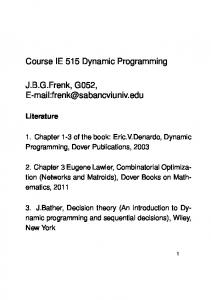
Fig. 2. Shoot-UFO-by-cannon task. Left: illustration of the task, right: graph-structured dynamical system of the task. Fig. 4. Neural network architecture used in this paper. It has two networks with the same input vector. The top part estimates an output vector, and the bottom part models prediction error and output noise. Both use ReLU as activation functions.

the forward and the backward propagations of the stochastic DDP. Refer to [18] for more details including comparisons with locally weighted regression.

Fig. 3. Result of the shoot-UFO-by-cannon task. Analytically obtained θ for each cannon is also plotted. There are three marker types: circle shows the selection is correct, cross shows the selection is wrong, and triangle shows an approximation (there is no analytical solution).

results. Note that there is no solution of θ for the cannon p1 and pex > 0.54, and for the cannon p2 and pex > 1.32. The marker shapes denote whether the cannon selection is correct or wrong. There were two mistakes. Since they were around the border where the optimal cannon changes, the th values of local optima were close. As a consequence, suboptimal solutions were chosen. When pex > 1.32, although there is no solution, Graph-DDP gives θ that maximizes R. V. L EARNING DYNAMICS When solving practical and complicated tasks such as manipulation of liquids, dynamical models are sometimes partially or totally unknown. For example in pouring, the flow dynamics are complicated to construct models analytically. In such situations, we learn models from samples obtained from practice. Specifically we use neural networks extended to be usable with stochastic DDP [18]. The extended neural networks are capable of: (1) modeling prediction error and output noise, (2) computing an output probability distribution for a given input distribution, and (3) computing gradients of output expectation with respect to an input. Since neural networks have nonlinear activation functions (in our case, rectified linear units, ReLU), these extensions were not trivial. In [18] we gave an analytic solution for them with some simplifications. Fig. 4 shows the neural network architecture used in this paper. We consider a mean model and an error model. The error model estimates output noise and prediction error. For a given set of samples of input {x} and output {y}, we train the mean model with a back propagation technique. Then we generate prediction errors (including output noise) {∆y} for training the error model. A special loss function is used. When a normal distribution x ∼ N (µ, Σ) is given as an input, our method computes E[y], cov[y], and the gradient ∂E[y] ∂µ analytically. Thus we can use the neural networks in

VI. T OY E XAMPLE (2) We apply Graph-DDP to a simplified pushing task where a target object position has a mixture-of-Gaussian uncertainty. This task was inspired by [21]. The task setup is illustrated in Fig. 5(left) where we consider a pushing task on a 2D plane. The target object is located at po , whose observation has a mixture-of-Gaussian distribution. An example physical situation is that a template matching algorithm detects multiple local optima of the matching function. Here we consider only a mixture of two Gaussian distributions, N (p1 , σ1 ), N (p2 , σ2 ), with fixed weights 0.5, 0.5 respectively. The pushing motion is predefined and parameterized with pm , θ, and m; the gripper is put at pm with the orientation θ, and moves forward with distance m. There are four possible cases of the result of the pushing motion as depicted in (a). . . (d) of Fig. 5(center). Only in cases (c) and (d), the target object moves, and only in (d) there is success (the object is pushed by the center of the gripper). Fig. 5(right) shows a graph-structured dynamical system to plan the pushing parameters. We use a bifurcation to represent multimodality (not a selection of actions); i.e. each branch corresponds with a Gaussian distribution, and FP s ⊤ (this is a gives the mixture weights: FP s () = [0.5, 0.5] constant). The edge dynamical systems Fgrasp1 and Fgrasp2 model the result of the pushing motion. We assume that these functions return ∆¯ p′1 and ∆¯ p′2 that denote the object position after the movement in the gripper coordinate system. Deriving these equations is trivial, but they have a nonlinearity; there are discrete changes in the dynamics as shown in (a). . . (d) of Fig. 5(center). We use a Taylor series expansion to obtain gradients of the dynamical systems, and compute the propagation of Gaussian distributions with local linear models. The reward is defined as: R = −1000∥∆¯ p′i ∥2 − 0.001m2 where i indicates 1 or 2. This reward means that we add a big penalty for ∥∆¯ p′i ∥ (the cases other than (d) of Fig. 5(center) are penalized), and a small penalty for gripper movement. We compare three cases: (1) using an analytical model, (2) using an analytical model without considering the Gaussian distributions (i.e. let σ1 and σ2 be zero), and (3) using neural network models for Fgrasp1 and Fgrasp2 . (2) is for verifying if the planned actions (1) consider the Gaussian distributions. Since the dynamical system contains discrete

Fig. 5. Push-under-uncertainty task. Left: illustration of the task, center: different results of pushing, right: graph-structured dynamical system of the task.

Fig. 7.

Fig. 6.

Result of the push-under-uncertainty task.

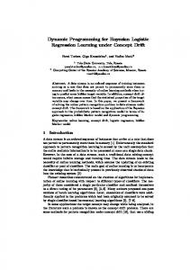
changes, the local linear model becomes inaccurate around the discontinuities, affecting DDP and the propagation of Gaussian distributions. We use our neural networks to see if these problems are reduced. As reported in [18], our stochastic neural networks give better predictions of output expectations and gradients especially when the approximated function includes discrete changes such as a step function. We randomly changed N (p1 , σ1 ) and N (p2 , σ2 ). The success rate of 100 trials are: (1) Analytical: 83, (2) Analytical (zero SD): 42, (3) Neural Networks: 96. Considering Gaussian distributions increases the success rate. Using neural network models also improves the success rate. Some examples are shown in Fig. 6. (a), (b), and (c) compare the three cases in the same situation. In (b), the gripper starts from the position where it touches both centers of Gaussian distributions p1 , p2 . The neural network model (c) gives intuitively correct plan compared to (a). (d), (e), and (f) are the results of the neural network model in different situations. These results would also be intuitively correct. Note the reason why the gripper movement is not on the line p1 -p2 in (d) and (f) would be due to the movement penalty. VII. S IMULATION E XPERIMENTS OF P OURING We explore the usefulness of Graph-DDP in a more complicated task, pouring. We extend the pouring simulator from our previous work [20], [18], to simulate a different viscosity of a material, and different mouth sizes of a source container. The purpose of the extension is to create a pouring task where different skills are necessary to generalize, similar to a real pouring task. Refer to the accompanying video. In Open Dynamics Engine (http://www.ode.org/), we simulate source and receiving containers, poured material, and a robot gripper grasping the source container as shown in Fig. 7(a). The gripper is modeled as fixed blocks around the source container. We can change the grasping position, but it does not affect the grasp quality. This gripper possibly pushes the receiving container during pouring.

(a) Pouring simulation setup. (b) Types of poured materials.

We simulate the poured material with many (100) spheres. Although each of the spheres is a rigid object, the entire group behaves like a liquid (no surface tension or adhesive effects). For simulating different types of materials, (1) we model a viscosity, and (2) we modify some contact model parameters, such as bouncing parameters. The viscosity is modeled by applying gravitational forces between spheres virtually. We use four types of materials: (wat): waterlike viscosity (non-viscous), (bnc): water-like viscosity (nonviscous) and high bouncing parameters, (vsc): large viscosity, and (vsc+): very large viscosity. The examples of these flows are shown in Fig. 7(b). If the mouth size of the source container is small enough, the flow of (vsc) and (vsc+) stop completely as the material is jammed around the mouth. Shaking the container can solve jamming. The diameter of each sphere is 0.05 (length unit in simulator; the gravity is 1.0), and the size of source mouth varies from 0.11 to 0.25. The behavior of pouring is designed with a state machine as illustrated in Fig. 8(top). The robot grasps the source container, moves it to somewhere close to the receiving container, moves it to the pouring location, and produces a flow with a selected skill. If the flow is not observed in a specific time, the robot moves the source container back and restarts from MoveToPour. This trial-and-error loop is repeated until the target amount is achieved or a specific duration passes. Fig. 8(bottom) models the dynamical system. The first two bifurcations are for penalizing the corresponding actions. Each flow control skill (tipping and shaking) is decomposed into two dynamical models (Fflowc ∗ and Famount ). This is because the decomposition makes the modeling easier as discussed in [20], and we can share a common model Famount . Fflowc ∗ estimates how the flow happens by the skill, and Famount estimates how the flow affects the poured and spilled amounts. Thus Fflowc ∗ depends on each skill but Famount can be common. We can train Famount with the samples of both tipping and shaking. The planning is done at the beginning and at the node n3 where the trial-and-error loop starts. Note that the dynamical system does not represent the trial-and-error loop because the planning assumes the pouring is completed with a single skill selection. We consider 19 types of state variables including container position, target amount, material property, mouth size, and flow position. The total dimensionality of the state vectors is 49. There are 6 types of action parameters including grasping, pouring position, and parameters for each skill. The total dimensionality of the action parameters is 8. Not

Fig. 8. State machine of pouring behavior (top) and its graph-structured dynamical system (bottom). F∗ denotes an edge dynamical system, and R∗ denotes a reward model.

all of the state vectors and action parameters are used in each dynamical system. The state vectors that do not affect a dynamical system are omitted. Consequently the dimensionalities of the edge dynamical systems vary up to 18. These are represented as a super-state-action dictionary. We use a reward function defined as follows: R = − 100(min(0, arcv − atrg ))2 − 10(max(0, aspill ))2 (8) − (max(0, arcv − atrg ))2 where arcv is an amount poured into the receiving container, atrg is a target amount, and aspill is a spilled amount. This reward function means that a big penalty is given for arcv < atrg since it is the first priority, a medium penalty is given for aspill > 0 since spillage should be avoided, and otherwise arcv being close to atrg is better. aspill ≥ is always satisfied in observation data, but the learned model might estimate aspill as a slight negative value. Thus we are using max(0, aspill ). A. On-line Learning and Learning Scheduling We use on-line learning, i.e. the robot plans actions with the latest models, and executes the actions and updates the models according to the results. If no model is available, the robot takes random actions. Each episode is defined as an entire pouring sequence including the trial-and-error loops. Through the preliminary experiments, we noticed that scheduling learning is useful to avoid local optima. We consider two types of scheduling. (1) Reward shaping: modifying the reward functions according to the number of episodes. (2) Setup scheduling: controlling the experimental setups. Note that an alternative approach to avoid local optima is increasing the exploration randomness, where these supervisory signals would be removed. Since we will use our method with real robots, here we explore efficient solutions. B. Experiments and Results First we consider a setup referred to as SETUP1: waterlike viscosity and high bouncing parameters (bnc), and wide mouth size of the source container (0.23). Note that tipping is the best skill in this setup. This is the same as our previous work [20], [18], but the difference is that these experiments have multiple skills. Thus the robot has to learn to select a skill as well as to tune skill parameters. We use pre-trained dynamical models other than Fflowc ∗ and Famount as these dynamical models are similar to those in [18] and can be learned easily. We compare two conditions: PT0-Rnone: no reward shaping, and PT0-Rtip:

Fig. 9. Poured amount per episode in SETUP1. A moving average filter with 5 episode window is applied.

tipping-biased reward shaping. The reward shaping of PT0Rtip is guiding the correct skill (tipping). More specifically, from 1st to 10th episode, we use R+10 if tipping is selected otherwise R, and after 11th episode, we use R. Fig. 9 shows the results of 10 runs. Each curve shows an average of poured amount per episode. The target amount is 0.3. The poured amount of PT0-Rtip is closer to the target than PT0-Rnone. In some runs of PT0-Rnone, shaking was chosen after learning. This was because shaking was good for early adaptation to the first objective, achieving arcv ≥ atrg , as defined in the reward Eq. (8). The excess amount is penalized, so tipping is better than shaking. But since that penalization is the third priority, there were a few runs where the robot tended to use shaking and dynamical models of tipping were not trained enough. The tippingbiased reward shaping was useful to handle this issue. It gained the tendency to select tipping in the early stage of learning. As the result, the average poured amount of PT0Rtip is smaller than that of PT0-Rnone. Next we investigate a setup referred to as SETUP2: large viscosity (vsc), and narrow mouth size of the source container (0.13). Shaking is the best skill in this setup. We compare three conditions: PT0-Rnone: Pre-trained dynamical models other than Fflowc ∗ and Famount , no reward shaping. PT1-Rnone: Pre-trained with SETUP1, no reward shaping. PT1-Rshake: Pre-trained with SETUP1, shaking-biased reward shaping. The shaking-biased reward shaping is that from 1st to 10th episode, we use R+10 if shaking is selected otherwise R, and after 11th episode, we use R. PT1-Rnone and PT1-Rshake are examples of the setup scheduling. Fig. 10 shows the learning curves, i.e. sum of rewards per episode, that are averages of 10 runs. PT1-Rnone and PT1-Rshake had more prior knowledge than PT0-Rnone. Especially Famount was learned in SETUP1, which would generalize in SETUP2. What PT1-Rnone and PT1-Rshake did not have are the training samples of Fflowc ∗ in SETUP2. Thus these converged faster than PT0-Rnone. The reward shaping was also useful in this setup. However since shaking is only the adequate solution in this setup (tipping does not work), all runs of PT1-Rnone (no reward shaping) did not converge to poor local optima. The variance of PT1-Rshake was increasing after 10th episode. This was because the reward-shaping changed. The reason why the variance of PT1-Rshake is greater than that of PT1-Rnone around the 10th episode is that tipping in this setup is not well-trained with PT1-Rshake in the 0th to 9th episodes because of the shaking-biased reward shaping. Thus in some runs, the robot tried tipping after the 10th episode.

Fig. 10. Learning curves (sum of rewards per episode) of SETUP2. A moving average filter with 5 episode window is applied.

Fig. 11. Learning curves (sum of rewards per episode) of the general pouring setup. A moving average filter with 5 episode window is applied.

Fig. 12. Skill selections in different situations (mouth size of source container, material type). The shape of the points show the skill (tipping, shaking). Setups for pre-training (SETUP1, SETUP2) are also shown. The size of point shows an error of poured amount.

Finally we explore the generalization ability of our method in a general pouring setup: four material types (wat, bnc, vsc, vsc+), and various mouth sizes of the source container (0.11 to 0.25). We consider three conditions including the setup scheduling. PT0-Rnone: Pre-trained dynamical models other than Fflowc ∗ and Famount , no reward shaping. PT1-Rnone: Pre-trained with SETUP1, no reward shaping. PT2-Rnone: Pre-trained with SETUP1 and SETUP2, no reward shaping. Fig. 11 shows the learning curves, i.e. sum of rewards per episode, which are averages of 10 runs. PT1-Rnone had more prior knowledge than PT0-Rnone, and PT2-Rnone had more than PT1-Rnone. The speed of the convergence seems to be proportional to the prior knowledge. Especially PT2-Rnone performs well in the early stages although it pre-trained only in specific situations (SETUP1, SETUP2). The variance of the learning curves is greater than that of Fig. 10. This is because in Fig. 11, the rewards from different setups are shown together. Although the three conditions converged to similar performance level, their details were slightly different. The graphs in Fig. 12 show which skill was selected in a situation. Each

graph plots 20 samples of all runs after convergence of learning curve. Each condition had a different tendency. In PT1-Rnone and PT2-Rnone, the skill selection was biased by the pre-training setups. In the viscous materials (vsc, vsc+) with a narrower mouth size, shaking was dominant regardless of the pre-training. In the highly bouncing material (bnc) case, tipping was dominant regardless of the pretraining. Since the learning curves in Fig. 11 converged to close values, there appears to be no convergence to poor local optima. VIII. C ONCLUSION We proposed a stochastic differential dynamic programming for graph-structured dynamical systems. We introduced the idea of frame-and-slots based on traditional artificial intelligence researches to represent a large state-action vector. The proposed method was applied to a simulated pouring task and showed that our method generalized over the material property (viscosity) and the source container shape (mouth size). Future work includes verifying our method in real pouring tasks by robots. R EFERENCES [1] A. Yamaguchi, C. G. Atkeson, and T. Ogasawara, “Pouring skills with planning and learning modeled from human demonstrations,” International Journal of Humanoid Robotics, vol. 12, no. 3, p. 1550030, 2015. [2] D. Mayne, “A second-order gradient method for determining optimal trajectories of non-linear discrete-time systems,” International Journal of Control, vol. 3, no. 1, pp. 85–95, 1966. [3] P. H. Winston, Artificial Intelligence (3rd Ed.). Addison-Wesley Longman Publishing Co., Inc., 1992. [4] Y. Pan and E. Theodorou, “Probabilistic differential dynamic programming,” in Advances in Neural Information Processing Systems 27. Curran Associates, Inc., 2014, pp. 1907–1915. [5] S. Levine and V. Koltun, “Variational policy search via trajectory optimization,” in Advances in Neural Information Processing Systems 26. Curran Associates, Inc., 2013, pp. 207–215. [6] M. D. Zeiler, “ADADELTA: an adaptive learning rate method,” ArXiv e-prints, no. arXiv:1212.5701, 2012. [7] J. Kober, J. A. Bagnell, and J. Peters, “Reinforcement learning in robotics: A survey,” International Journal of Robotics Research, vol. 32, no. 11, pp. 1238–1274, 2013. [8] E. Theodorou, J. Buchli, and S. Schaal, “Reinforcement learning of motor skills in high dimensions: A path integral approach,” in ICRA’10, may 2010, pp. 2397–2403. [9] J. Kober and J. Peters, “Policy search for motor primitives in robotics,” Machine Learning, vol. 84, no. 1-2, pp. 171–203, 2011. [10] S. Schaal and C. Atkeson, “Robot juggling: implementation of memory-based learning,” in ICRA’94, 1994, pp. 57–71. [11] J. Morimoto, G. Zeglin, and C. Atkeson, “Minimax differential dynamic programming: Application to a biped walking robot,” in the IEEE/RSJ International Conference on Intelligent Robots and Systems (IROS’03), vol. 2, 2003, pp. 1927–1932. [12] I. Lenz, R. Knepper, and A. Saxena, “DeepMPC: Learning deep latent features for model predictive control,” in Robotics: Science and Systems (RSS’15), 2015. [13] E. Magtanong, A. Yamaguchi, K. Takemura, J. Takamatsu, and T. Ogasawara, “Inverse kinematics solver for android faces with elastic skin,” in Latest Advances in Robot Kinematics, Innsbruck, Austria, 2012, pp. 181–188. [14] E. W. Aboaf, C. G. Atkeson, and D. J. Reinkensmeyer, “Task-level robot learning,” in IEEE International Conference on Robotics and Automation, 1988, pp. 1309–1310. [15] E. W. Aboaf, S. M. Drucker, and C. G. Atkeson, “Task-level robot learning: juggling a tennis ball more accurately,” in the IEEE International Conference on Robotics and Automation, 1989, pp. 1290–1295. [16] A. Yamaguchi and C. G. Atkeson, “Model-based reinforcement learning with neural networks on hierarchical dynamic system,” in the Workshop on Deep Reinforcement Learning: Frontiers and Challenges in IJCAI’16, 2016. [17] V. Mnih, K. Kavukcuoglu, D. Silver, et al., “Human-level control through deep reinforcement learning,” Nature, vol. 518, no. 7540, pp. 529–533, 2015. [18] A. Yamaguchi and C. G. Atkeson, “Neural networks and differential dynamic programming for reinforcement learning problems,” in ICRA’16, 2016. [19] S. J. Russell and P. Norvig, Artificial Intelligence: A Modern Approach. Prentice-Hall, Inc., 1995. [20] A. Yamaguchi and C. G. Atkeson, “Differential dynamic programming with temporally decomposed dynamics,” in Humanoids’15, 2015. [21] M. C. Koval, N. S. Pollard, and S. S. Srinivasa, “Pre- and postcontact policy decomposition for planar contact manipulation under uncertainty,” The International Journal of Robotics Research, vol. 35, no. 1-3, pp. 244–264, 2016.