Differentially Private Bayesian Learning on Distributed Data

Differentially Private Bayesian Learning on Distributed Data

arXiv:1703.01106v1 [stat.ML] 3 Mar 2017

1

Mikko Heikkil¨a1 , Yusuke Okimoto2 , Samuel Kaski3 , Kana Shimizu2 and Antti Honkela1,4,5 Helsinki Institute for Information Technology (HIIT), Department of Mathematics and Statistics, University of Helsinki 2 Department of Computer Science and Engineering, Waseda University 3 HIIT, Department of Computer Science, Aalto University 4 HIIT, Department of Computer Science, University of Helsinki 5 Department of Public Health, University of Helsinki

Abstract Many applications of machine learning, for example in health care, would benefit from methods that can guarantee privacy of data subjects. Differential privacy (DP) has become established as a standard for protecting learning results, but the proposed algorithms require a single trusted party to have access to the entire data, which is a clear weakness. We consider DP Bayesian learning in a distributed setting, where each party only holds a single sample or a few samples of the data. We propose a novel method for DP learning in this distributed setting, based on a secure multi-party sum function for aggregating summaries from the data holders. Each data holder adds their share of Gaussian noise to make the total computation differentially private using the Gaussian mechanism. We prove that the system can be made secure against a desired number of colluding data owners and robust against faulting data owners. The method builds on an asymptotically optimal and practically efficient DP Bayesian inference with rapidly diminishing extra cost.

1

Introduction

Data privacy has gained an increasing amount of attention in recent years. The importance of rigorous data privacy mechanisms has been accentuated by several well-known examples of supposedly privatised data sets being used to identify individuals therein, such as (Barbaro and Zeller, 2006) and (Narayanan and Shmatikov, 2008).

Differential privacy (DP) (Dwork et al., 2006; Dwork and Roth, 2014) is theoretically the best-founded way of protecting privacy. It gives mathematically provable guarantees against breaches of individual privacy that are robust even against attackers with access to additional side information. The DP field is already well-established and a substantial amount of work has been done in the past decade. Many important techniques regularly used for solving machine learning problems have been considered under the privacy constraint. General principles have been proposed e.g. for maximum likelihood estimation (Smith, 2008), empirical risk minimisation (Chaudhuri et al., 2011) and Bayesian inference (e.g. Dimitrakakis et al., 2013; Foulds et al., 2016; Honkela et al., 2016; J¨alk¨o et al., 2016; Park et al., 2016; Wang et al., 2015; Zhang et al., 2016). There are DP versions of most popular machine learning methods including linear regression (Honkela et al., 2016; Zhang et al., 2012), logistic regression (Chaudhuri and Monteleoni, 2009), support vector machines (Chaudhuri et al., 2011), and deep learning (Abadi et al., 2016). The standard methods assume that some trusted party has unrestricted access to all data in order to add the necessary amount of noise needed for the privacy guarantees. This is a highly restrictive assumption for many applications. In contrast, it is desirable to develop methods for a distributed setting where no such trusted aggregator exists. A naive approach to distributed DP learning would require each party to add sufficient noise to effectively mask any single sample in the small data set they hold, which will require adding excessive noise. In this paper we introduce a general strategy for privacypreserving Bayesian learning in the distributed setting with

minimal overhead. Our method builds on the asymptotically optimal sufficient statistic perturbation mechanism (Foulds et al., 2016; Honkela et al., 2016) and shares its asymptotic optimality. The method is based on a new DP secure multi-party communication (SMC) algorithm called Master-Compute algorithm (MCA) for achieving DP in the distributed setting. We demonstrate its performance on DP Bayesian inference using a linear regression model problem as an example.

ciphertext leaks no information about the plaintext (Goldwasser and Micali, 1984), and have the property that it enables computing Enc(m1 + m2 ) without knowing m1 , m2 and sk, given two ciphertexts Enc(m1 ) and Enc(m2 ) of messages m1 and m2 . Hereafter, we denote the property by Enc(m1 ) ⊕ Enc(m2 ). From among such schemes, we use the Paillier cryptosystem (Paillier, 1999).

1.1

We propose a general approach that combines SMC with DP Bayesian learning methods, originally introduced for the trusted aggregator setting, to achieve DP Bayesian learning in the distributed setting.

Differential privacy, originally introduced by Dwork et al. (2006), is a method that gives strict, mathematically provable guarantees against intrusions on individual privacy. The main idea in DP is to add random noise to a data set in such a way as to mask the influence any single individual can have on the results calculated from the data.

To guarantee privacy securely and with maximal utility, we introduce a novel algorithm, MCA, for answering sum queries without a trusted aggregator. Our method uses Paillier homomorphic encryption scheme for secure aggregation together with a Gaussian mechanism for differential privacy.

Formally, we consider randomised algorithms on adjacent data sets, where adjacency means that the data sets differ by a single element, i.e., the two data sets have the same number of samples, but they differ on a single one. In this work we utilise a relaxed version of DP called (, δ)-differential privacy, as in Definition 2.4 of Dwork and Roth (2014).

Compared to the existing DP-SMC methods, our algorithm is faster and scales well with the number of data holders, while still offering good security properties. Set against the trusted aggregator setting, the method achieves almost the same noise level for any practical number of data holders.

Definition 2.1. A randomised algorithm A is (, δ)differentially private, if for all S ⊆ Range (A) and all adjacent data sets D, D0 ,

Our method can guarantee privacy against colluding data holders and fault tolerance against data holders dropping out without adding new communication rounds or major key management problems.

The parameters  and δ in Definition 2.1 control the privacy guarantee:  tunes the amount of privacy (smaller  means stricter privacy), while δ can be interpreted as the proportion of probability space where the privacy guarantee may break down.

Our Contribution

The method can also support dynamic joins and leaves. In this case users can drop out of the scheme while others join it between the communication rounds without the need for running complicated setup routines. We demonstrate the general framework and the MCA performance empirically by considering a problem of Bayesian linear regression in the distributed setting.

2 2.1

Background

2.2

P (A(D) ∈ S) ≤ exp()P (A(D0 ) ∈ S) + δ.

There are several established mechanisms for ensuring DP. We use the Gaussian mechanism (Theorem 3.22 in Dwork and Roth, 2014). The theorem says that given a query f with l2 -sensitivity ∆2 (f ), adding noise distributed as N (0, σ 2 ) to each output component guarantees DP, when σ 2 > 2 ln(1.25/δ)(∆2 (f )/)2 .

(1)

Here, the l2 -sensitivity on adjacent data sets D, D0 is defined as

Cryptographic primitives for secure multi-party computation

In this paper, we perform secure multi-party computation for calculating aggregated results based on homomorphic encryption. More formally, we use an additively homomorphic public-key encryption scheme (KeyGen; Enc; Dec). KeyGen is a key generation algorithm that creates a pair of a public key pk and a secret key sk. Enc(m) denotes a ciphertext obtained by encrypting message m under pk and Dec(c) denotes the decryption result of ciphertext c under sk. This scheme should be semantically secure, that is, a

Differential Privacy

∆2 (f ) =

sup x∈D,x0 ∈D 0

||f (x) − f (x0 )||2 .

(2)

We consider alternatives to the Gaussian mechanism in Section 8. 2.3

Differentially private Bayesian learning

Bayesian learning provides a natural complement to DP because it can inherently handle uncertainty, including that introduced because of DP (Williams and McSherry, 2010), and it provides a flexible framework for data modelling.

Three distinct types of mechanisms for DP Bayesian inference have been proposed:

Clients

1. Drawing a small number of samples from the posterior or an annealed posterior (Dimitrakakis et al., 2014; Wang et al., 2015);

Broadcast public key to everyone

Enc(zi + ηi )

Master key manager

2. Perturbing the sufficient statistics of an exponential family model (Foulds et al., 2016; Honkela et al., 2016; Park et al., 2016); and P

3. Perturbing the gradients in optimisation of variational inference (J¨alk¨o et al., 2016). For models where it applies, the sufficient statistic perturbation approach is asymptotically efficient (Foulds et al., 2016; Honkela et al., 2016), unlike the posterior sampling mechanisms. The sufficient statistic perturbation (#2) and gradient perturbation (#3) mechanisms are of similar form in that the DP mechanism ultimately computes a perturbed sum z=

N X

zi + η

(3)

i=1

over quantities zi computed for different samples i = 1, . . . , N , where η denotes the noise injected to ensure the DP guarantee. For sufficient statistic perturbation (Foulds et al., 2016; Honkela et al., 2016; Park et al., 2016), the zi are the sufficient statistics of a particular sample, whereas for gradient perturbation (J¨alk¨o et al., 2016), the zi are the clipped per-sample gradient contributions. When a single party holds the entire data set, the sum z in Eq. (3) can be computed easily. Next we will consider calculating the perturbed sum of Eq. (3) securely in the distributed setting.

3

Secure and Private Learning

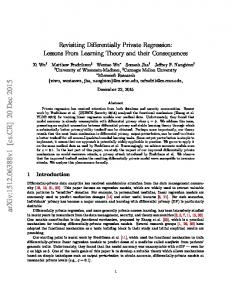
Let us assume there are N data holders (called clients in the following), who each hold a single data sample. We would like to use the aggregate data for learning, but the clients do not want to reveal their data as such to anybody else. The main problem with the distributed setting is that if each client uses a trusted aggregator DP technique separately, the noise η in Eq. (3) is added by each client, increasing the total noise level by a factor of N , effectively reducing to naive input perturbation. To reduce the noise level without compromising on privacy, the individual data samples need to be combined without revealing them directly to anyone. For solving this problem, we present our Master-Compute Algorithm.

z i + ηi

Individual encryption

i zi

+ ηi

Compute untrusted aggregator ⊕i Enc(zi + ηi )

DP result

Figure 1: Schematic diagram of the Master-Compute Algorithm. Red refers to encrypted values, blue to unencrypted DP values.

3.1

Master-Compute Algorithm

We assume that the final query results can be partitioned into a sum over the results of some operations performed on the individual data samples, as in Eq. (3). For the adversary model, we assume the clients are honestbut-curious, i.e., they will take a peek at other people’s data if given the chance, but they will follow the protocol. We additionally assume at most T clients may collude to break the privacy, either by revealing the noise they add to their data samples or by abstaining from adding the noise in the first place. In order to add the correct amount of noise while avoiding revealing the unperturbed data to any single party, we combine a homomorphic encryption scheme with the Gaussian mechanism for DP as illustrated in Fig. 1. The idea is that each individual client adds a small amount of Gaussian noise to his data, so that when the individual data points are aggregated, the total noise is also Gaussian with variance that sums up to the correct level. The details of the noise scaling along with a proof that the result is DP are presented in Section 3.2. Using homomorphic encryption the necessary summations can be done under encryption without revealing the unperturbed data. Since the standard Paillier scheme only works for integers, the values are represented in fixed-point format. Our approach relies on two distinct entities called Master and Compute. Master is responsible for handling the cryptographic keys and for distributing the final unencrypted DP results, while Compute does the actual summations under encryption without access to the private key (see Algo-

rithm 1 and Figure 1). 3.2

Privacy of the mechanism

4.5 4.0

σj2 ≥

Proof. Using the property that a sum of independent Gaussian variables is another Gaussian with variance equal to the sum of the component variances, we can divide the total noise equally among the N clients. This gives the mini2 mum variance σpart = σj2 /N when adding the noise in N separate pieces on line 2 of Algorithm 1. However, in the distributed setting even with all honestbut-curious clients, there is an extra scaling factor needed

3.0 2.5

1.5 1.0

0

20

40 60 Number of clients

80

100

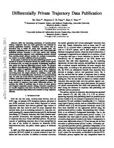
Figure 2: Extra scaling factor needed for the noise in the distributed honest-but-curious-clients setting with colluding clients as compared to the trusted aggregator setting.

compared to the standard DP. Since each client knows the noise values she adds to the data, she can also remove them from the aggregate values. In other words, privacy has to be guaranteed by the noise the remaining N − 1 clients add to the data. If we further assume the possibility of T colluding clients, then the noise from N − T − 1 clients must be sufficient to guarantee the privacy. The additional noise factor c0 has to satisfy the inequality N −T X−1 i=1

2 2 c0 σj,part ≥ σj,std

2 2 ⇔ (N − T − 1)c0 σj,part ≥ N σj,part ,

(4) (5)

N which clearly holds when c0 ≥ N −T −1 . The variance each individual client uses for generating the independent Gaussian noise that guarantees DP is therefore

N σ2 , N − T − 1 j,std

2 where N is the number of clients and σj,std is the variance of the noise in the standard Gaussian mechanism given in Eq. (1).

3.5

2.0

In order to guarantee that the sum-query results returned by Algorithm 1 are DP, we need to show that the variance of the aggregated Gaussian noise is large enough. Theorem 1 (Distributed Gaussian mechanism). If at most T clients collude or drop out of the protocol, the sumquery result returned by Algorithm 1 is differentially private, when the variance of the added noise σj2 fulfils

Scaling factor needed to guarantee privacy Number of colluding clients T=0 T=5 T=10

5.0

Scaling factor

Algorithm 1 Master-Compute Algorithm for secure distributed summation Input: Distributed Gaussian mechanism noise variances σj2 , j = 1, . . . , d (public); Number of parties N (public); d-dimensional vectors zi held by clients i ∈ {1, . . . , N } PN Output: Differentially private sum i=1 zi + η, where ηj ∼ N (0, σj2 ) 1: Master generates a pair of secret and public keys (sk, pk), and shares the public key pk to Compute and to each of the clients 2: Each client simulates ηi ∼ N (0, diag(σj2 /N )) and calculates mi = zi + ηi , where i ∈ {1, . . . , N } is the ID of the client. The client then
encrypts the noisy sums: Enc(mi,1 ), . . . , Enc(mi,d ) and sends them to Compute. 3: After receiving the encrypted noisy values from all of the clients, Compute PNcalculates an encrypted noisy aggregate sum Enc( i=1 mi,k ) = Enc(m1,k ) ⊕ · · · ⊕ Enc(mN,k ) and stores it as ck for k = 1, . . . , d. It then sends (c1 , . . . , cd ) to Master. 4: After receiving (c1 , . . . , cd ), Master obtains DP
PN PN sums by computing i=1 mi,1 , . . . , i=1 mi,d Dec(c1 ), . . . , Dec(cd ) and distributes them to interested parties.

σj2 ≥

N σ2 . N − T − 1 j,std

(6)

In the case of all honest-but-curious clients, T = 0. The extra scaling factor increases the variance of the distributed noise, but this factor quickly approaches 1 as the number of clients increases, as shown in Figure 2. 3.3

Fault Tolerance

The same strategy used to protect against colluding clients can also be used for creating a fault-tolerant version of the method. With the all honest-but-curious clients and T = 0, if one client fails to send his data then the summed up

noise variance is not sufficient to guarantee privacy, and consequently the algorithm needs to be started again from the beginning with the corrected noise variance. When T > 0, at most T clients in total can drop or collude and the scheme will still remain private. 3.4

Computational scalability

There are two main bottlenecks in Algorithm 1: all the clients need to send their individual results to Compute, which then has to calculate the final sums under encryption. A naive implementation with d-dimensional data, assuming each of the N clients simply sends d encrypted numbers to Compute which then sums them up one by one, has linear complexity O(dN ). The server-side computations parallelise trivially up to d ways. For further parallelisation with N > d d-dimensional inputs, we could create a binary tree of Compute nodes such that each node calculates the sum of two vectors and sends the results to a higher level Compute node. In this case we could use dN/2i e nodes for the ith layer, where i = 1 is the input layer, giving complexity of O(d log N ). 3.5

Security of the mechanism

In order to guarantee the security of the scheme, Master and Compute must not collude. The scheme could be made more resistant against such collusion using the binary tree aggregation outlined above as individual Compute nodes would then only have access to either very few samples or aggregates. We assume the data providers have an interest in the results and hence they will not attempt to pollute the results with invalid values.

4

DP Bayesian learning on distributed data

In order to perform DP Bayesian learning securely in the distributed setting, we use the MCA Algorithm 1 to compute the required data summaries that are of the form shown in Eq. (3). In this Section we consider how to combine this scheme with concrete DP learning methods introduced for the trusted aggregator setting. These methods provide a wide range of possibilities for performing DP Bayesian learning securely with distributed data. They also exemplify the basic steps needed in order to convert a trusted aggregator setting method to the distributed setting. The distributed algorithm is most straightforward to apply to the sufficient statistic perturbation method of Foulds et al. (2016) and Honkela et al. (2016) for exact and approximate posterior inference on exponential family models. Foulds et al. (2016) and Honkela et al. (2016) use Lapla-

cian noise to guarantee -DP, which is a stricter form of privacy than the (, δ)-DP used in Algorithm 1 Dwork and Roth (2014). We consider here only (, δ)-DP version of the method, and discuss the possible Laplace noise mechanism further in Section 8. The model training in this case is done in a single iteration, so a single application of Algorithm 1 is enough for learning. 4.1

Distributed Bayesian Linear Regression with Data Projection

We consider next the Bayesian linear regression (BLR) with data projection method in detail in the distributed setting. The standard BLR model depends on the data only through sufficient statistics, and the distributed data posterior inference approach discussed in Section 4 can be used in a straightforward manner to fit the model by running a single round of Algorithm 1. The more efficient BLR of Honkela et al. (2016) introduces data projection to reduce the data range by non-linearly projecting all data points inside stricter bounds. Since the DP noise level is determined by the sensitivity of the data, reducing the sensitivity by limiting the data range translates into less added noise. By selecting the bounds suitably, we only need to introduce a little bias while significantly decreasing the variance from DP. In the distributed setting, the data projection needs to run an additional round of Algorithm 1 and use a part of the privacy budget to estimate data standard deviations (stds). However, as shown by the test results (see Figure 4), this still achieves significantly better utility with a given privacy level. The method is described in detail in Algorithm 2. It estimates the DP sufficient statistics needed to fit a BLR model with data projection securely in the distributed setting. Full source code is freely available through GitHub1 and a more detailed description can be found in the supplement. The assumed bounds in Step 1 are needed for the initial estimation of standard deviations for scaling. These would typically be available from general knowledge of the data. The projection in Step 1 ensures the privacy of the scheme even if the bounds are invalid for some samples. We determine the optimal projection thresholds pj in Step 4 using the same general approach as Honkela et al. (2016): we create an auxiliary data set of equal size as the original with data generated as xi ∼ N (0, Id )

(7)

yi |xi ∼ N (xTi β, λ).

(9)

β ∼ N (0, λ0 I)

(8)

We then perform grid search on the auxiliary data to find optimal thresholds by calculating the projection with different thresholds and comparing the prediction performances. 1

Available on publication

Algorithm 2 Distributed linear regression with projection Input: Number of clients N (public), data and target values (xij , yi ), j = 1, . . . , d held by clients i ∈ {1, . . . , N }, assumed data and target bounds (−cj , cj ), j = 1, . . . , d + 1 (public), privacy budget (, δ) (public), Output: DP BLR sufficient statisticsP of projected Pmodel N N data N xx ˆ = i=1 x ˘Ti x ˘i +η (1) , N xy ˆ = i=1 x ˘Ti y˘i + (2) η 1: Each client projects his data to the assumed bounds (−cj , cj ) ∀j, giving bounded data (˜ xij , y˜i ), j = 1, . . . , d 2: Divide the privacy budget into equal shares for each dimension iter = /(d(d + 1)/2 + 2d + 1), δiter = δ/(d(d + 1)/2 + 2d + 1) 3: Calculate marginal std estimates σ (1) , . . . , σ (d+1) from marginal var estimates produced by running Algorithm 1 with zi = (˜ x2i1 , . . . , x ˜2id , y˜i2 ) and the distributed Gaussian mechanism variances calculated using the assumed bounds and privacy budget (iter , δiter ) 4: Estimate optimal projection thresholds pj , j = 1, . . . , d + 1 as fractions of std on auxiliary data 5: Each client projects his data to the estimated optimal bounds (−pj σ (j) , pj σ (j) ), j = 1, . . . , d + 1, giving projected data (˘ xi1 , . . . , x ˘id , y˘i ) 6: Aggregate the unique terms in the DP sufficient statistics by running Algorithm 1 with zi = (˘ x2i1 , x ˘i1 x ˘i2 , . . . , x ˘2id , x ˘i1 y˘i , . . . , x ˘id y˘i ) and the corresponding distributed Gaussian mechanism noise variances calculated using the estimated optimal bounds and privacy parameters (iter , δiter ) 7: Combine the DP result vectors from Algorithm 1 into the symmetric d × d matrix and d-dimensional vector of DP sufficient statistics

4.2

Distributed differentially private variational inference

We can apply the same distributed algorithms also for DP variational inference J¨alk¨o et al. (2016); Park et al. (2016). These methods rely on possibly clipped gradients or expected sufficient statistics calculated from the data. Typically, each training iteration would use only a mini-batch instead of the full data. To use variational inference in the distributed setting, an arbitrary party keeps track of the current (public) model parameters and the privacy budget, and asks for updates from the clients. Since this model trainer does not have any privileged access to the private data, the clients could also do the model training jointly, provided that there is an agreed upon method for selecting the mini-batches available. At each iteration, the model trainer selects a random mini-

batch of fixed public size from the available clients and sends them the current model parameters. The selected clients then make use of Algorithm 1 to send the requested data to the model trainer, i.e., they calculate the clipped gradients or expected sufficient statistics using their data, add noise to the values scaled reflecting the batch size, encrypt them, and send them to the Compute. The model trainer receives the decrypted DP sums from the Master and updates the model parameters.

5

Experimental Setup

We demonstrate the secure DP Bayesian learning scheme in practice by testing the performance of the BLR with data projection, the implementation of which was discussed in Section 4.1, along with the MCA (Algorithm 1) in the all honest-but-curious clients distributed setting (T = 0). For the MCA our primary interest is the performance of the algorithm. In the case of BLR implementation, we are interested in comparing the distributed algorithm to the trusted aggregator version as well as comparing the performance of the straightforward BLR to the variant using data projection, since it is not clear a priori if the extra cost in privacy, necessitated by the projection in the distributed setting, is offset by the reduced noise level. We use simulated data for the MCA scalability testing, and real data for the BLR tests. As real data, we use the Wine Quality (Cortez et al., 2009) and Abalone data sets from the UCI repository2 . We split the Wine Quality data to two parts for red wines and white wines. The data sets are assumed to be zero-centred. This assumption is not crucial but is done here for simplicity; non-zero data means can be estimated like the marginal standard deviations at the cost of some added noise (see Section 4.1). For estimating the marginal std, we also need to assume bounds for the data. For unbounded data, we can enforce arbitrary bounds simply by projecting all data inside the chosen bounds, although very poor choice of bounds will lead to poor performance. With real distributed data, the assumed bounds could differ from the actual data range. In the tests we simulate this effect by scaling the data to [−5, 5] and then assuming bounds of [−7.5, 7.5], i.e., the assumed bounds clearly overestimate the true bounds, which adds more noise to the results. The actual scaling chosen here is arbitrary. The optimal projection thresholds are searched for using 12 repeats on a grid with 20 points between 0.1 and 2.1 times the std of the auxiliary data set. In the search we use one common threshold for all data dimensions and a separate one for the target. For accuracy measure, we use prediction accuracy on a sep2

http://archive.ics.uci.edu/ml/datasets.html

10 0

Compute wall time for summations under encryption

Wall time (s)

10 -1

Number of dimensions 9 35 104

10 -3

32

100 Number of clients repeats=5

317

1000

Figure 3: Minimum of Compute wall times over 5 repeats. The purely serial implementation scales well with a reasonable number of clients and dimensions as shown here. However, a more complicated parallelised implementation would be advantageous for significantly larger inputs.

arate test data set. The size of the test set in Figure 4 is 500 for red wine, 1000 for white wine, and 1000 for abalone data. We compare the median performance measured on mean absolute error over 40 runs using input perturbation Dwork et al. (2006) and the trusted aggregator setting as baselines.

6

Related Work

To the best of our knowledge, there is no prior work on secure DP Bayesian statistical inference in the distributed setting. The existing prior works mainly focus on answering simple database queries and on distributed classification.

10 -2

10 -410

7

Results

Figure 3 shows the Compute wall-clock times with several numbers of clients and dimensions. The serial implementation is clearly sufficiently fast for these cases but for larger examples the parallel implementations outlined in Sec. 3.4 may be necessary. Comparing the results on predictive error with and without projection (top row and bottom row in Fig. 4, respectively), it is clear that despite incurring extra privacy cost for having to estimate the marginal standard deviations, using the projection can improve the results markedly with a given privacy budget. The results also demonstrate that compared to the trusted aggregator setting, the extra noise added due to the distributed setting with honest-but-curious clients is insignificant in practise as the results of the distributed and trusted aggregator algorithms are effectively indistinguishable. We further tested the performance of the same alternatives when changing the size of the data set with white wine data. The results (Supplementary Figure 1) show that the prediction accuracy does not significantly depend on the number of samples in the range [500, 4000].

Rastogi and Nath (2010) present a method for distributed DP time series analysis by answering simple queries on Fourier transform coefficients using a distributed Laplace mechanism. The distributed Laplace mechanism could be used instead of MCA in our work if pure -DP is required. Pathak et al. (2010) present a method for aggregating classifiers in a DP manner, but their approach is sensitive to the number of parties and sizes of the data sets held by each party and cannot be applied in a completely distributed setting. Rajkumar and Agarwal (2012) improve upon this by an algorithm for distributed DP stochastic gradient descent that works for any number of parties. The fundamentally iterative nature of their stochastic gradient descent means the method cannot be combined with the asymptotically optimal sufficient statistic perturbation for DP Bayesian inference. Hamm et al. (2016) present an alternative aggregation method that uses an auxiliary public data set to improve the performance. There is a wealth of literature on secure distributed computation of DP sum queries as reviewed by Goryczka and Xiong (2015). Shi et al. (2011) present several DP definitions and results for the distributed setting. They also present the idea of noise scaling to achieve collusion resistance that is similar to our approach, although Shi et al. (2011) require that the colluding data holders still add noise according to the scheme, while we assume more adversarial colluders who can leave the noise out completely if they so choose. ´ and The same idea of noise scaling was also used by Acs Castelluccia (2011), Chan et al. (2012) and Goryczka and Xiong (2015). However, unlike the method of Shi et al. (2011), all of these schemes can also provide fault tolerance by the addition of a separate recovery round after data holder failures. Compared to the previous collusion-resistant and fault´ and Castelluccia (2011); Chan et al. tolerant methods Acs (2012); Goryczka and Xiong (2015), the MCA effectively saves one round of communication and avoids more complicated key management issues by assuming that the key management and the untrusted aggregation are done separately. It can also support dynamic joins and leaves with very light overhead, since it does not require any pairwise secret key exchanging. Finally, Wu et al. (2016) present several proofs related to the SMC setting and introduce a protocol for generating approximately Gaussian noise in a distributed manner. Com-

DDP proj DDP

input perturbed 5

2.5

NP proj NP

proj TA

(b) Abalone data set, distributed DP with projection and non-projected methods

3.0 2.5

2.0

2.0 MAE

2.5

1.5 1.0

NP proj NP

proj TA

0.5

0.03 0.1 0.32 1.0 3.16 10.0 31.62 100.0 epsilon d=11, sample size=2000, repeats=40, δ = 0.0001

(c) White wine data set, distributed DP with projection and non-projected methods

2.0

NP proj NP

proj TA

proj DDP

1.8 1.6 1.4

1.5

0.5

1.5

proj DDP

1.2 1.0 0.8

1.0 0.03 0.1 0.32 1.0 3.16 10.0 31.62 100.0 epsilon d=11, sample size=1000, repeats=40, δ = 0.0001

input perturbed

1.0 0.03 0.1 0.32 1.0 3.16 10.0 31.62 100.0 epsilon d=8, sample size=2000, repeats=40, δ = 0.0001

proj DDP

DDP proj DDP

2.0

3

0.03 0.1 0.32 1.0 3.16 10.0 31.62 100.0 epsilon d=11, sample size=1000, repeats=40, δ = 0.0001

NP TA

2.5

1

(a) Red wine data set, distributed DP with projection and non-projected methods

MAE

3.0

2

1.0

0.5

input perturbed

MAE

MAE

MAE

1.5

3.0

DDP proj DDP

4

2.0

0.5

NP TA

MAE

3.0

NP TA

0.6 0.03 0.1 0.32 1.0 3.16 10.0 31.62 100.0 epsilon d=8, sample size=2000, repeats=40, δ = 0.0001

0.4

0.03 0.1 0.32 1.0 3.16 10.0 31.62 100.0 epsilon d=11, sample size=2000, repeats=40, δ = 0.0001

(d) Red wine data set, all methods with pro- (e) Abalone data set, all methods with pro- (f) White wine data set, all methods with jection jection projection

Figure 4: Median of the Bayesian linear regression model predictive accuracy on several UCI data sets with error bars denoting the interquartile range. NP refers to non-private version, TA to the trusted aggregator setting, DDP to the distributed scheme. The performance of the distributed methods is indistinguishable from the corresponding undistributed TA algorithms and the projection can clearly be beneficial for prediction performance. pared to their protocol, our method of noise addition is considerably simpler and faster, and produces exactly instead of approximately Gaussian noise.

8

Discussion

We have presented a general framework for performing DP Bayesian learning securely in a distributed setting. Our method combines a practical SMC method for calculating secure sum queries with efficient Bayesian DP learning techniques adapted to the distributed setting. DP methods are based on adding sufficient noise to effectively mask the contribution of any single sample. The extra loss in accuracy due to DP tends to diminish as the number of samples increases, and efficient DP estimation methods converge to their non-private counterparts as the number of samples increases (Foulds et al., 2016; Honkela et al., 2016). A distributed DP learning method can significantly help in increasing the number of samples because data held by several parties can be combined thus helping make DP learning significantly more effective.

Considering the DP and the SMC components separately, it is clear that the choice of method to use for each subproblem can be made largely independently. Assessing these separately, we can therefore easily change the privacy mechanism from the Gaussian used in Algorithm 1 to the Laplace mechanism, e.g. by utilising one of the distributed Laplace noise addition methods presented by Goryczka and Xiong (2015) to obtain a pure -DP method. The secure sum algorithm in our method can also be easily replaced with a more complicated and secure variant if more security is needed. While the noise introduced for DP will not improve the performance of an otherwise good learning algorithm, a DP solution to a learning problem can yield better results if the DP guarantees allow access to more data than without privacy. Our distributed method can further help make this more efficient by securely and privately combining data from multiple parties.

Acknowledgements This work was funded by the Academy of Finland [Centre of Excellence COIN, 283193 to S.K., 294238 to S.K., 292334 to S.K., 278300 to A.H., 259440 to A.H. and 283107 to A.H.] and the Japan Agency for Medical Research and Development (AMED).

References Martin Abadi, Andy Chu, Ian Goodfellow, H. Brendan McMahan, Ilya Mironov, Kunal Talwar, and Li Zhang. Deep learning with differential privacy. In Proc. CCS 2016, 2016. doi: 10.1145/2976749.2978318. arXiv:1607.00133 [stat.ML]. ´ and Claude Castelluccia. I have a DREAM! Gergely Acs (DiffeRentially privatE smArt Metering). In Tom´asˇ Filler, Tom´asˇ Pevn´y, Scott Craver, and Andrew Ker, editors, Information Hiding: 13th International Conference, IH 2011, Prague, Czech Republic, May 18-20, 2011, Revised Selected Papers, pages 118– 132. Springer Berlin Heidelberg, Berlin, Heidelberg, 2011. ISBN 978-3-642-24178-9. doi: 10.1007/ 978-3-642-24178-9 9. URL http://dx.doi.org/ 10.1007/978-3-642-24178-9_9. Michael Barbaro and Tom Zeller. A face is exposed for AOL searcher No. 4417749. New York Times, August 2006. T. H. Hubert Chan, Elaine Shi, and Dawn Song. Privacypreserving stream aggregation with fault tolerance. In Angelos D. Keromytis, editor, Financial Cryptography and Data Security: 16th International Conference, FC 2012, Kralendijk, Bonaire, Februrary 27March 2, 2012, Revised Selected Papers, pages 200– 214. Springer Berlin Heidelberg, Berlin, Heidelberg, 2012. ISBN 978-3-642-32946-3. doi: 10.1007/ 978-3-642-32946-3 15. URL http://dx.doi. org/10.1007/978-3-642-32946-3_15.

Support Systems, 47(4):547–553, 2009. doi: 10.1016/j. dss.2009.05.016. Christos Dimitrakakis, Blaine Nelson, Zuhe Zhang, Aikaterini Mitrokotsa, and Benjamin Rubinstein. Bayesian differential privacy through posterior sampling. 2013. arXiv 1306.1066 [stat.ML], updated 2016. Christos Dimitrakakis, Blaine Nelson, Aikaterini Mitrokotsa, and Benjamin I. P. Rubinstein. Robust and private Bayesian inference. In ALT 2014, volume 8776 of Lecture Notes in Computer Science, pages 291–305. Springer Science + Business Media, 2014. Cynthia Dwork and Aaron Roth. The algorithmic foundations of differential privacy. Foundations and Trends in Theoretical Computer Science, 9(3-4):211–407, 2014. ISSN 1551-305X. doi: 10.1561/0400000042. URL http://dx.doi.org/10.1561/0400000042. Cynthia Dwork, Frank McSherry, Kobbi Nissim, and Adam Smith. Calibrating noise to sensitivity in private data analysis. In Shai Halevi and Tal Rabin, editors, Theory of Cryptography: Third Theory of Cryptography Conference, TCC 2006, New York, NY, USA, March 4-7, 2006. Proceedings, pages 265–284. Springer Berlin Heidelberg, Berlin, Heidelberg, 2006. ISBN 978-3-540-32732-5. doi: 10.1007/11681878 14. URL http://dx.doi.org/10.1007/11681878_14. James Foulds, Joseph Geumlek, Max Welling, and Kamalika Chaudhuri. On the theory and practice of privacy-preserving Bayesian data analysis. In Proceedings of the Thirty-Second Conference on Uncertainty in Artificial Intelligence, UAI’16, pages 192–201, Arlington, Virginia, United States, March 2016. AUAI Press. ISBN 978-0-9966431-15. URL http://dl.acm.org/citation.cfm? id=3020948.3020969. arXiv:1603.07294 [cs.LG]. Shafi Goldwasser and Silvio Micali. Probabilistic encryption. J. Comput. Syst. Sci., 28(2):270–299, 1984.

Slawomir Goryczka and Li Xiong. A comprehensive comKamalika Chaudhuri and Claire Monteleoni. Privacyparison of multiparty secure additions with differential preserving logistic regression. In D. Koller, privacy. IEEE Transactions on Dependable and Secure D. Schuurmans, Y. Bengio, and L. Bottou, editors, Computing, 2015. doi: 10.1109/TDSC.2015.2484326. Advances in Neural Information Processing SysJihun Hamm, Paul Cao, and Mikhail Belkin. Learning pritems 21, pages 289–296. Curran Associates, Inc., vately from multiparty data. In ICML, 2016. 2009. URL http://papers.nips.cc/paper/ 3486-privacy-preserving-logistic-regression. Antti Honkela, Mrinal Das, Onur Dikmen, and Samuel pdf. Kaski. Efficient differentially private learning improves drug sensitivity prediction. arXiv:1606.02109, 2016. Kamalika Chaudhuri, Claire Monteleoni, and Anand D. Sarwate. Differentially private empirical risk minimization. J. Mach. Learn. Res., 12:1069–1109, July 2011. ISSN 1532-4435. URL http://dl.acm. org/citation.cfm?id=1953048.2021036. Paulo Cortez, Ant´onio Cerdeira, Fernando Almeida, Telmo Matos, and Jos´e Reis. Modeling wine preferences by data mining from physicochemical properties. Decision

Joonas J¨alk¨o, Onur Dikmen, and Antti Honkela. Differentially private variational inference for non-conjugate models. arXiv:1610.08749, 2016. Arvind Narayanan and Vitaly Shmatikov. Robust deanonymization of large sparse datasets. In Proceedings of the 2008 IEEE Symposium on Security and Privacy, SP ’08, pages 111–125, Washington, DC, USA, 2008.

IEEE Computer Society. ISBN 978-0-7695-3168-7. doi: 10.1109/SP.2008.33. URL http://dx.doi.org/ 10.1109/SP.2008.33.

analysis under differential privacy. PVLDB, 5(11):1364– 1375, 2012. URL http://vldb.org/pvldb/ vol5/p1364_junzhang_vldb2012.pdf.

Pascal Paillier. Public-key cryptosystems based on composite degree residuosity classes. In Proceedings of the 17th international conference on Theory and application of cryptographic techniques, EUROCRYPT’99, pages 223–238, Berlin, Heidelberg, 1999. Springer-Verlag. ISBN 3-540-65889-0. URL http://dl.acm.org/ citation.cfm?id=1756123.1756146.

Zuhe Zhang, Benjamin Rubinstein, and Christos Dimitrakakis. On the differential privacy of Bayesian inference. In Proc. AAAI 2016, 2016. arXiv:1512.06992 [cs.AI].

Mijung Park, James Foulds, Kamalika Chaudhuri, and Max Welling. Variational Bayes in private settings (VIPS). arXiv:1611.00340, 2016. Manas A. Pathak, Shantanu Rane, and Bhiksha Raj. Multiparty differential privacy via aggregation of locally trained classifiers. In Proceedings of the 23rd International Conference on Neural Information Processing Systems, NIPS’10, pages 1876–1884, USA, 2010. Curran Associates Inc. URL http://dl.acm.org/ citation.cfm?id=2997046.2997105. Arun Rajkumar and Shivani Agarwal. A differentially private stochastic gradient descent algorithm for multiparty classification. In AISTATS, pages 933–941, 2012. Vibhor Rastogi and Suman Nath. Differentially private aggregation of distributed time-series with transformation and encryption. In Proceedings of the 2010 ACM SIGMOD International Conference on Management of Data, SIGMOD ’10, pages 735–746, New York, NY, USA, 2010. ACM. ISBN 978-1-4503-0032-2. doi: 10.1145/1807167.1807247. URL http://doi.acm. org/10.1145/1807167.1807247. E. Shi, T. Chan, E. Rieffel, R. Chow, and D. Song. Privacypreserving aggregation of time-series data. Proceedings of NDSS, 2011. Adam Smith. Efficient, differentially private point estimators. September 2008. arXiv:0809.4794 [cs.CR]. Yu-Xiang Wang, Stephen E. Fienberg, and Alexander J. Smola. Privacy for free: Posterior sampling and stochastic gradient Monte Carlo. In Proc. ICML 2015, pages 2493–2502, 2015. URL http://jmlr.org/ proceedings/papers/v37/wangg15.html. O. Williams and F. McSherry. Probabilistic inference and differential privacy. In Adv. Neural Inf. Process. Syst. 23, 2010. Genqiang Wu, Yeping He, Jingzheng Wu, and Xianyao Xia. Inherit differential privacy in distributed setting: Multiparty randomized function computation. In 2016 IEEE Trustcom/BigDataSE/ISPA, pages 921– 928, Aug 2016. doi: 10.1109/TrustCom.2016.0157. arXiv:1604.03001 [cs.CR]. Jun Zhang, Zhenjie Zhang, Xiaokui Xiao, Yin Yang, and Marianne Winslett. Functional mechanism: Regression

Supplement This supplement contains a more detailed presentation of the Bayesian linear regression with projection discussed in the main text and some additional test results. In the following, we denote the ith observation in d dimensional data by xi , the scalar target values by yi , and the whole d + 1−dimensional dataset by Di = (xi , yi ). We assume all column-wise expectations to be zeroes for simplicity. For n observations, we denote P the sufficient statisPn n tics by nxx ¯ = i=1 xTi xi and nxy ¯ = i=1 xTi yi .

For the regression, we assume that

yi |xi ∼N (xTi β, λ), i = 1, . . . , n β ∼N (0, λ0 I),

(10) (11)

where we want to learn the posterior over β, and λ, λ0 are hyperparameters (set to 1 in the tests). The posterior can be solved analytically to give ˆ β|y, x ∼ N (ˆ µ, Λ), ˆ = λ0 I + λnxx, Λ ¯ ˆ −1 (λnxy). µ ˆ=Λ ¯

(12)

(14)

The amount of noise each client needs to add to the output depends partly on the sensitivity of the function in question. Assuming that dimension j is bounded on an interval (−bj , bj ), and that the neighbouring datasets D, D0 differ only at element t ∈ {1, . . . , n}, the sensitivity for the (j, k), j 6= k element in the sufficient statistics is ∆2 (f ) = =

sup x∈D,y∈D 0

sup x∈D,y∈D 0

=

sup x∈D,y∈D 0

≤ ||2bj bk ||2

The DP sufficient statistics are given by nxx ˆ = nxx ¯ + xx , nxy ˆ = nxy ¯ + xy , where xx , xy consist of suitably scaled Gaussian noise added independently to each dimension. In total, there are d(d + 1)/2 + d parameters in the combined sufficient statistic, since nxx ¯ is a symmetric matrix. The main idea in the data projection is simply to project the data into some reduced range. Since the noise level is determined by the sensitivity of the data, reducing the sensitivity by limiting the data range translates into less added noise. With projection threshold c, the kth dimension of the data (k) xi is given by (k)

This gives us the projection thresholds in terms of std for each dimension. We then estimate the marginal std for each dimension by using Algorithm 1 (in the main text), to fix the actual projection thresholds. For this the data is assumed to lie on some known bounded interval. In practice, the assumed bounds need to be based on prior information. In case the estimates are negative due to noise, they are set to small positive constants.

(13)

The predicted values from the model are yˆj = x0j µ ˆ.

x˘i (k) = max(−c, min(xi , c)).

bounds, we first find an optimal projection threshold by grid search on an auxiliary dataset, that is generated from a BLR model similar to the regression model defined above.

(15)

This data projection obviously discards information, but in various problems it can be beneficial to disregard some information in the data in order to achieve less noisy estimates of the model parameters. From the bias-variance trade-off point of view, this can be seen as increasing the bias while reducing the variance. The optimal trade-off then depends on the actual problem. To run Algorithm 2 (in the main text), we need to assume projection bounds (cj , dj ) for each dimension j ∈ {1, . . . , d + 1} for the data D. In the paper we assume bounds of the form (−cj , cj ). To find good projection

= 2bj bk .

||f (x) − f (y)||2 ||

X

(j) (k)

xi xi

i (j) (k)

||xt xt

−

(16) X

i (j) (k)

(j) (k)

yi yi ||2 (17)

− yt yt ||2

(18) (19) (20)

In contrast, with the projected data the corresponding sensitivity is readily calculated to be ∆2 (f ) ≤ 2cj ck , which shows how the projection reduces the noise level when cj ck < bj bk . For j = k, the same calculation gives ∆2 (f ) ≤ b2j for the non-projected and ∆2 (f ) ≤ c2j for the projected data. Additional Results Figure 5 shows the prediction error with fixed privacy parameters and changing sample size. The results support our claim that the projection method can improve predictive performance.

4.0

NP TA

DDP proj DDP

input perturbed

3.5

MAE

3.0 2.5 2.0 1.5 1.0 0.5

500

1000

2000 3000 4000 sample size d=11, repeats=40, ² = 1, δ = 1e-05

(a) White wine dataset, distributed DP with projection and non-projected methods

0.9

NP proj NP

proj TA

proj DDP

0.8

MAE

0.7 0.6 0.5 0.4

500

1000

2000 3000 4000 sample size d=11, repeats=40, ² = 1, δ = 1e-05

(b) White wine dataset, all methods with projection

Figure 5: Median prediction error with IQR for UCI white wine dataset.