arXiv:cond-mat/9610158v1 22 Oct 1996. Diffusion and localization in chaotic billiards. Fausto Borgonovi[a,c,d], Giulio Casati[b,c,e] Baowen Li[f,g].
Diffusion and localization in chaotic billiards Fausto Borgonovi[a,c,d], Giulio Casati[b,c,e] Baowen Li[f,g] [a]
arXiv:cond-mat/9610158v1 22 Oct 1996
Dipartimento di Matematica, Universit` a Cattolica, via Trieste 17, 25121 Brescia, Italy [b] Universit` a di Milano, sede di Como, Via Lucini 3, Como, Italy [c] Istituto Nazionale di Fisica della Materia, Unit` a di Milano, via Celoria 16, 22100 Milano, Italy Istituto Nazionale di Fisica Nucleare, Sezione di Pavia[d] , Sezione di Milano[e] , [f ] Department of Physics and Centre for Nonlinear and Complex Systems, Hong Kong Baptist University, Hong Kong [g] Center for Applied Mathematics and Theoretical Physics, University of Maribor, Krekova 2, 2000 Maribor, Slovenia We study analytically and numerically the classical diffusive process which takes place in a chaotic billiard. This allows to estimate the conditions under which the statistical properties of eigenvalues and eigenfunctions can be described by Random Matrix Theory. In particular the phenomenon of quantum dynamical localization should be observable in real experiments. PACS numbers: 05.45.+b, 05.20.-y
is not applicable. We consider the motion of a particle having mass m, velocity ~v and elastically bouncing inside the stadium shown in Fig 1. We denote with R the radius of the semicircles and with 2a the length of the straight segments. The total energy is E = m~v 2 /2. The statistical properties of the billiard are controlled by the dimensionless parameter ǫ = a/R and, for any ǫ > 0, the motion is ergodic, mixing and exponentially unstable with Lyapunov exponent Λ which, for small ǫ, is given by [6] Λ ∼ ǫ1/2 . For the analysis of classical dynamics, a typical choice of canonical variables is (s, vt ) where s measures the position along the boundary of the collision point and vt is the tangent velocity. These variables however, are quite difficult to treat from the quantum point of view. For this purpose it is convenient instead to consider l, the angular momentum calculated with respect to the center of the stadium, and the angle θ which describes, together with r(θ), the position of the particle in the usual polar coordinates. It is important to stress that with this choice of variables, the invariant measure dµ = dsdvt is preserved only to order ǫ, that is dµ = dsdvt = dθdl + o(ǫ) At a given energy E, the angular momentum must √ satisfy the relation |l| < lmax = (R + a) 2Em. It is therefore convenient to introduce the rescaled quantity L = l/lmax. Then the classical motion takes place on the cylinder 0 ≤ θ < 2π, −1 < L < 1. It is expected that for ǫ 1/a. This implies E > Ep = h ¯ 2 /2ma2 which is the energy necessary to confine a quantum particle inside a box of length a. Using the well known Weyl formula for the total number of states with energy less than E [3]
On the other side the change in θ, to zero order, is given by : ¯ ∆θ = θ¯ − θ = π − 2 arcsin(L)
(2)
According to a standard procedure [7] we introduce a ¯ θ) in such a way that the map generating function G(L, defined by L=
∂G θ¯ = ¯ ∂L
∂G ; ∂θ
(3)
coincides with ∆L at first order in ǫ and with ∆θ at zero-th order. The generating function is given by: ¯ θ) = (θ + π)L ¯ −2 G(L,
Z
¯ L
¯ cos θ| dL arcsin L + ǫg(L)| hN (E)i ≈
(4)
�
R ¯h
�2
E
(7)
where A is the area of a quarter of billiard, and keeping only the leading term, we obtain that in order to be in a non perturbative regime we have to consider level numbers
¯ = 2sign(L)(1 ¯ −L ¯ 2 )1/2 . The generated (imwhere g(L) plicit) area–preserving map is ¯ = L − 2ǫ sin θsign(cos θ)sign(L)(1 ¯ ¯ 2 )1/2 L −L ′ ¯ ¯ ¯ θ = θ + π − 2 arcsin(L) + ǫg (L)| cos θ|
mA 1 E≈ m 8 2π¯h2
(5)
N ≫ Np ≃
By taking the local approximation in the angular momentum, the map (5) writes : p ¯ = L − 2ǫ sin θsign(cos θ)sign(L) ¯ 1 − L2 L 0 (6) ¯ θ¯ = θ + π − 2 arcsin(L)
1 16ǫ2
(8)
We call Np perturbative border. According to the well known arguments [11], above the perturbative border (8) quantum diffusion in angular momentum takes place with a diffusion coefficient close to the classical one. This diffusion proceeds up to a time τB ∼ Def f /¯h2 after which diffusion will be suppressed by quantum interference. This time is related to the uncertainty principle. Namely, for times less than τB the discrete spectrum is not resolved and the quantum motion mimics the classical diffusive motion [11,12]. Here Def f = D0 ǫ5/2 2mER2 is the classical diffusion coefficient in real (not scaled) angular momentum. The nature of the quantum steady state will depend crucially on the ergodicity parameter [12]
which remains area–preserving and can be easily iterated (here L0 is the initial angular momentum). The agreement of map (6) with the true dynamics can be numerically checkedpand it is shown in Fig.2 where we ¯ − L)/(2ǫ 1 − L2 ) against θ. Points repreplot L∗ = (L 0 sent billiard dynamics while the full line is the function f (θ) = − sin θsign(cos θ). Notice that the function f (θ) is periodic of period π and has a discontinuity at θ = π/2. This gives to the map (6) a structure very close to the sawtooth map which is known [8] to be chaotic and diffusive with a diffusion rate D which, for small values of the kick strength ǫ, is given by D ∼ ǫ5/2 . This behaviour, according also to our numerical computations, appears to be generic for maps which have such type of discontinuity. We may proceed now to a numerical investigation of the diffusive process. To this end we consider a distribution of particles with given initial L0 and random phases θ in the interval (0, 2π) and integrate the classical equations of motion inside the billiard. In Figs. 3a,b we present the behaviour of ∆L2 = hL2 i − hL0 i2 as a function of the number of collisions n and the distribution function fn (L) at fixed n as a function of (L − L0). As it is seen, ∆L2 grows diffusively and the distribution function is in good agreement with a Gaussian [9]. In particular the dependence D = D(ǫ) of the diffusion coefficient
λ2 =
τB τE
(9)
2 where τE = lmax /Def f ≃ 2mER2 /Def f is the ergodic relaxation time. For λ ≪ 1 the quantum steady state is localized while for λ ≫ 1 we have quantum ergodicity. The critical value λ = 1 leads to lmax ¯h = Def f that is E = Eerg = ǫ−5 D0−2 ¯h2 /2mR2 . We then have :
N = Nerg ≃
1 16D02 ǫ5
(10)
It follows that only for N > Nerg there is quantum ergodicity and therefore one expects statistical properties of eigenvalues and eigenfunctions to be described by 2
RMT. Instead for N < Nerg , even if N ≫ Np , namely very deep in quasiclassical regions, √ statistical properties will depend on parameter λ = D0 8N ǫ5 and not separately on ǫ or N . For example, the nearest neighbour levels spacing distribution P (s) will approach e−s when λ ≪ 1. We have tested this prediction by numerically computing the level spacing distribution for different values of ǫ and N . One example is shown in Fig.5 for which N ≫ Np but since λ ≪ 1 the distribution P (s) is close to e−s as expected. Similar behaviour is expected for other quantities such as the two points correlation function, the probability distribution of eigenfunctions, etc. The numerical computations are based on the improved plane wave decomposition method [13]. The accuracy of eigenvalues is better than one percent of the mean level spacing. We also compared the results with the semiclassical formula in order to check that there are no missing levels. Notice that the effect predicted here is entirely due to quantum dynamical localization and bears no relation with the existence of bouncing ball orbits. The same behaviour will be present in chaotic billiards in which no family of periodic orbits exists. The effects of quantum localization discussed here should be observable in microwave or sound wave experiment. Finally we would like to mention that the diffusive process in angular momentum and the corresponding suppression caused by quantum mechanics may be of interest for a new class of optical resonators which have been recently proposed [5]. We are indebted to R.Artuso, B.V.Chirikov, I.Guarneri and D.Shepelyansky for valuable discussions and suggestions. B. Li is grateful to the colleagues of the University of Milano at Como for their hospitality during his visit. His work is supported in part by the Research Grant Council RGC/96-97/10 and the Hong Kong Baptist University Faculty Research Grant FRG/95-96/II-09 and FRG/95-96/II-92.
[4]
[5]
[6] [7] [8] [9]
[10] [11] [12]
[13]
[1] G.Casati, B.V.Chirikov, J.Ford and F.M.Izrailev, Lectures Notes in Physics 93 (1979) 33, Springer Verlag ( see also Ref. 12 ). [2] E. J. Galvez, B. E. Sauer, L. Moorman, P. M. Koch and D. Richards, Phys. Rev. Lett. 61, (1988) 2011; J.E.Bayfield, G.Casati, I.Guarneri and D.Sokol Phys. Rev. Lett. 63, (1989) 364; M.Arndt, A.Buchleitner, R.N.Mantegna, H.Walther Phys. Rev. Lett. 67, (1991) 2435; F.L.Moore, J.C. Robinson, C.F.Bharucha, B.Sundaram and M.G.Raizen Phys. Rev. Lett. 75, (1995) 4598. [3] O.Bohigas, Proceedings of the 1989 Les Houches Summer School on “Chaos and Quantum Physics”, ed.
3
M.J.Giannoni, A.Voros and J.Zinn-Justin, p.89, Elsevier Science Publisher B.V., North–Holland, (1991) G.Casati, B.V.Chirikov, I.Guarneri and F.M.Izrailev Phys.Rev.E 48, (1993) R1613; G.Casati, B.V.Chirikov, I.Guarneri and F.M.Izrailev preprint Budker INP 95-98 Novosibirsk, (1995). J.U.Nockel and A. D. Stone in Optical Processes in Microcavities, edited by R. K. Chang and A. J. Campillo (World Scientific Publishing Co., 1995), and A.Mekis, J.U.N¨ ockel, G.Chen, A.D.Stone and R.K.Chang, Phys. Rev. Lett. 75, (1995) 2682. In these papers it is proposed that the spoiling of high-Q whispering gallery modes in deformed dielectric spheres can be understood as a transition to chaotic ray dynamics (in deformed circular billiards) which can no longer be confined by total internal reflection. G.Benettin, Physica 13D, (1984) 211. A.J.Lichtenberg and M.A.Lieberman, Regular and Stochastic Motion, Applied Math. Series 38 (1983). I.Dana, N.W.Murray and I.C.Percival Phys.Rev.Lett. 62 (1989) 233. It may be interesting to remark that the diffusion coefficient computed in terms of the number of collisions, appears to depend on the initial value of angular momentum L. This is due to the fact that the mean free path depends on angular momentum and that even though the system is ergodic, ergodicity is not uniform in time. If one computes the diffusion coefficient in terms of real physical time then the dependence on the initial L0 value disappears. For the above reasons map (6) approximate the real dynamics provided L0 is not too close to 1. B.V.Chirikov preprint 90-116 Novosibirsk, (1990). B.V.Chirikov, F.M.Izrailev and D.L.Shepelyansky, Sov. Scient. Rev. 2C, 209 (1981). G.Casati and B.V.Chirikov , ”Quantum Chaos”, Cambridge University press, (1995); Physica D, 86 (1995) 220. E.Heller, in Proceeding of the 1989 Les Houches Summer School on ”Chaos and Quantum Physics”, ed. M. Giannoni, A.Voros, J.Zinn-Justin, B.Li and M.J.Robnik J.Phys. A 27 (1994) 5509, and E.Vergini and M.Saraceno, Preprint 1994, ”Calculation by scaling of highly excited states of billiards”
r
R
θ
R+a
*
FIG. 1. The Bunimovich stadium with radius R and straight segments 2a ; the variables (r(θ), θ) indicate the position of the point along the boundary.
*
FIG. 3. Diffusion in angular momentum for the billiard with ǫ = 0.01. Here an ensemble of 104 particles was chosen with initial L0 = 0 and random position along the boundary. a) ∆L2 as a function of the number of collisions n; the dashed line is the best fit and gives D = ∆L2 /n = 1.5 · 10−5 . b) Distribution function after n = 500 collisions averaged over the last 50 collisions. The full line is the best fitting Gaussian with average −0.016 and variance 0.1.
*
FIG. 2. Comparison between the billiard dynamics and the map (6). Here we plot the variable L∗ versus θ (see text). Points are obtained from numerically integrating the motion of one particle in the billiard for 100 iterations, starting from L0 = 0 and a random position along the boundary, while the full line is the function f (θ) (see text). Here ǫ = 0.01. The points not belonging to the curve are due to collisions with one of the straight lines; this occurrence is outside the approximation of map (6).
4
* *
FIG. 5. Level spacings distribution computed on 2000 levels in the interval 51000 < N < 53000 for ǫ = 0.01 (a) and ǫ = 0.1 (b). In the first case (a) Np ≃ 600 and Nerg ≃ 2.8·108 and therefore Np ≪ N ≪ Nerg . The value λ ≃ 0.01 of the ergodicity parameter accounts for the fact that the numerically computed P (s) is close to e−s (full curve). In the case (b) one has Nerg ≃ 2.8 · 103 ≪ N and therefore, as expected, the distribution P (s) is close to Wigner-Dyson (dotted curve).
2
FIG. 4. Diffusion coefficient D = ∆L /n for the stadium (full circles) as a function of ǫ. Open circles indicate the diffusion rate obtained from the map (6). The line is obtained by the usual best fitting procedure to the true dynamics (full circles) and gives D = D0 ǫ2.5 with D0 = 1.5.
5