Draft Version 7/3/12, Copyright CPA Canadian Journal of Experimental Psychology: http://www.apa.org/journals/cep/ This copy may not exactly replicate the final version published in the CPA journal. It is not a copy of record.
Diffusion versus Linear Ballistic Accumulation: Different models for response time with different conclusions about psychological mechanisms? Andrew Heathcote1 & Brett Hayes2 1The University of Newcastle, Australia 2The University of New South Wales, Australia
Corresponding Author: Andrew Heathcote School of Psychology, Psychology Building The University of Newcastle, Callaghan, Australia, 2308 Ph: 61-‐2-‐49216778 Email:
[email protected] Keywords: Response time, Mathematical Psychology, Practice, Lexical Decision
1
Two similar classes of evidence-‐accumulation model have dominated theorizing about rapid binary choice: diffusion models and racing accumulator pairs. Donkin et al. (2011) examined mimicry between the Ratcliff diffusion (RD: Ratcliff & Smith, 2004) and the linear ballistic accumulator (LBA: Brown & Heathcote, 2008), the two least similar models from each class that provide a comprehensive account of a set benchmark phenomena in rapid binary choice. Where conditions differed only in the rate of evidence accumulation (the most common case in past research), simulations showed the models supported equivalent psychological inferences. In contrast, differences in two other parameters of key psychological interest, response caution (the amount of information required for a decision), and non-‐decision time, traded-‐off when fitting one model to data simulated from the other, implying the potential for divergent inferences about latent cognitive processes. However, Donkin et al. did not find such inconsistencies between fits of the RD and LBA models in a survey of data sets from paradigms using a range of experimental manipulations. We examined a further data set, collected by Dutilh et al. (2009), which used a manipulation not surveyed by Donkin et al.; practice. Dutilh et al.’s RD model fits indicated that practice had large effects on all three types of parameters. We show that the in this case the LBA provides a different and simpler account of practice effects. Implications for evidence accumulation modelling are discussed.
2
Measurements related to performance in choice tasks underpin many psychological investigations. When choices are rapid (i.e., made in a few seconds or less), not only the response chosen, but also response time (RT), is of interest. This is particularly the case where choices are scored for accuracy, as inferences about psychological processes based on either accuracy or RT alone are confounded when participants engage in a speed-‐accuracy trade-‐off (e.g., increasing accuracy by increasing RT). The most successful method of addressing such confounding is to fit the data with an evidence-‐accumulation model, as inferences based on model-‐parameter estimates address potential speed-‐accuracy trade-‐off. A second advantage of this approach is that it titrates the time required to complete decision and non-‐decision processes. However, there are several different evidence accumulation models that provide apparently equally comprehensive accounts of the benchmark phenomena common to a range of rapid choice paradigms (Ratcliff & Smith, 2004; Brown & Heathcote, 2005, 2008). This led Donkin, Brown, Heathcote and Wagenmakers (2011) to question whether there was potential for different models to support conflicting inferences about psychological processes. Simulation results showed there was indeed room for such ambiguity, but reassuringly, they failed to find any evidence that it occurred in a survey of empirical data sets. However, we show here that ambiguity does occur in data collected by Dutilh, Vandekerckhove, Tuerlinckx and Wagenmakers (2009) on the effect of practice on binary choice in the lexical decision task (i.e., deciding if a string of letters forms a word) and discuss the implications.
3 Evidence Accumulation Models
Until relatively recently, successful evidence accumulation models assumed that choice errors are mainly caused by random fluctuations in evidence from moment-‐to-‐moment during a choice trial (Ratcliff & Smith, 2004). Accumulating (i.e., summing) evidence over time averages out this stochastic noise, increasing accuracy. Speed-‐accuracy trade-‐off is explained by changes in response caution, which determines the evidence boundary required to trigger a response. A higher boundary requires a longer period of accumulation to obtain the required evidence, increasing both RT and accuracy. However, such models have been shown to be unable to provide a comprehensive account of rapid choice performance without the addition of extra sources of noise due to trial-‐to-‐trial fluctuations (Ratlciff & Rouder, 1998). For example, the widely applied Ratcliff Diffusion (RD) model assumes trial-‐to-‐trial noise in the mean rate of evidence accumulation (v) and the accumulation starting point (z, i.e., the evidence total before stimulus-‐based accumulation begins). Brown (2002) investigated whether all three types of noise are necessary in another comprehensive model, Usher and McClelland’s (2001) leaky competitive accumulator (LCA). Surprisingly, he found only the trial-‐to-‐trial noises were required to provide the same comprehensive account of benchmark phenomena as the original LCA model and the RD model. For example, speed-‐accuracy trade-‐ off can occur due to trial-‐to-‐trial noise because longer accumulation overcomes random biases caused by starting-‐point noise. Brown and Heathcote (2005a)
4
called this non-‐stochastic LCA, the Ballistic Accumulator1. Brown and Heathcote (2008) showed that an even simpler version, the Linear Ballistic Accumulator (LBA), which drops non-‐linear leakage and competition effects in the LCA, also provides a comprehensive account. These simplifications have the advantage that they make it possible to derive an easily computed likelihood function, facilitating applications of the LBA (e.g., Eidels, Donkin, Brown & Heathcote, 2010; Farrell, Ludwig, Ellis & Gilchrist, 2009; Farrell, Ludwig, Ellis & Gilchrist, 2010; Forstmann, Schäfer, Anwander, Neumann, Wagenmakers, Bogacz, Turner, 2010; Forstmann, Dutilh, Brown, Neumann, von Cramon, Ridderinkhof & Wagenmakers, 2008; Ho, Brown & Serences, 2009; Ludwig, Ellis, Hardwicke & Gilchrist, in press). Donkin et al. (2011) compared the two least similar of the models just discussed, the RD and LBA, by fitting one to data simulated from the other. For simulated experimental manipulations affecting only the rate parameter the models were in qualitative agreement. In contrast, simulated RD response caution manipulations affected not only LBA response caution, but also its rate and non-‐decision time parameters. Conversely, simulated LBA response caution manipulations affected RD non-‐decision time estimates as well as response caution. However, Donkin et al. did not find any evidence for similar disagreements in fits of both models to a range of empirical data sets. Here we extend Donkin et al.’s (2011) search for different psychological conclusions from fits of the two models to the same empirical data set. We focus on a data set collected by Dutilh et al.’s (2009) for several reasons. First, they 1The term ballistic was used to indicate the deterministic nature of accumulation within a trial,
and does not indicate that a change of input during a trial has no effect accumulation (see Brown & Heathcote, 2005b).
5
experimentally manipulated response caution. Second, they collected a very large amount of data for each participant, which facilitates model fitting. Third, their psychological focus, practice effects, caused large changes in the three primary RD model parameters, rate, response caution and non-‐decision time. Below, we review details of Dutilh et al.’s (2009) experiment, model and findings. We then propose an LBA model and report the results of fitting it to the same data. Our aim was to determine whether an LBA model that provides a good description of Dutilh et al.’s (2009) data could imply different parameter-‐based inferences about the psychological processes underpinning practice effects. Dutilh et al.’s (2009) Model and Results Figure 1 illustrates Dutilh et al.’s (2009) model of the lexical decision task. In this task participants must decide as quickly as possible whether a letter-‐string stimulus makes up a word or is a non-‐word. Evidence is represented by vertical position and time by horizontal position. Increases in evidence favour word decisions and decreases in evidence favour non-‐word decisions. Stimulus encoding is assumed to take a time te, after which evidence accumulation commences at a starting value of z. The start point lies between an evidence boundary of 0 for a non-‐word decision and a for a word decision; a is called a boundary separation parameter. The decision is unbiased if the staring point lies half way between these boundaries (i.e., z = a/2). The irregular line in Figure 1 represents an instance of the evolution of evidence over time. The fluctuations are caused by the addition to a constant evidence input provided by the encoded stimulus of normally distributed moment-‐to-‐moment noise, with mean zero and standard deviation s. A decision
6
occurs when evidence first crosses a decision boundary (dotted horizontal lines in Figure 1). A word decision is made for a crossing at a and a non-‐word decision for a zero crossing. Figure 1 shows a word decision at time te+td. The irregular evidence path illustrates how moment-‐to-‐moment noise can lead to a speed-‐ accuracy trade-‐off; if the lower boundary were raised sufficiently (or equivalently if the starting point were sufficiently biased toward non-‐words) a fast non-‐word decision would have been made. Once the boundary crossing occurs a response is made after response production time tr, so RT = te + td + tr. Once the stimulus is encoded it provides evidence at a mean rate vW for words and vN for non-‐words. In Figure 1 the stimulus is a word, which produces a positive mean rate indicated by the large arrow. The mean rate varies between trials according to a normal distribution. Ratcliff (1978) proposed this type of trial-‐to-‐trial variability in applying the diffusion model to recognition memory for words. In this application, where a different item is used on every trial, trial-‐ to-‐trial rate variability can be interpreted as being caused by item differences. However, even when stimuli are identical within a condition, the RD model estimates substantial trial-‐to-‐trial rate variability, so factors such as fluctuations in attention are also a likely cause. The starting point also varies between trials according to a uniform distribution with mean z and width sz, reflecting trial-‐to-‐ trial fluctuations in bias. Sequential effects due to prior trials are one likely cause of this type of variability. Dutilh et al. (2009) also assumed uniform trial-‐to-‐trial noise in non-‐decision time (i.e., the sum of stimulus encoding and response production times), centred on a mean value ter with width st. The inclusion of this fourth source of noise is justified by Ratcliff, Gomez and McKoon’s (2004) modeling of word frequency
7
effects in a lexical decision task. They found it necessary to add ter variability in order to account for the effect of word frequency using only mean rate differences. In particular, the addition was necessary to capture the effect of word frequency on the leading edge of the distribution of RT for correct responses, as measured by the 10th pecentile (i.e., the RT below which the fastest 10% of responses occurred). Without ter variability the frequency-‐related change in the 10th percentile was too small, as rate differences have only small effects on the RD leading edge. Because ter variability widens the fast tail of the RT distribution, it increased the rate difference effect to a level that Ratcliff et al. deemed sufficient to account for the word frequency effect. Design and Data Each of Dutilh et al.’s (2009) four participants performed 25 blocks of 400 trials. Practice was divided into five separate sessions of five blocks, and participants responded to the same 200 words and 200 non-‐words in each block. Two participants (A1 and A2) were instructed to emphasize accurate responding, whereas the other two (S1 and S2) were asked to emphasize response speed. These instructions were reinforced by feedback after each trial: for speed “too slow!” for responses less than 750ms and for accuracy “error” after errors, with “too fast” after responses less than 200ms in both cases. Such instruction manipulations reliably induce a speed-‐accuracy trade-‐off, and are modelled as selectively influencing boundary separation (Ratcliff & Rouder, 1998). Figure 2 shows results (circles joined by dotted lines) for the performance measures on which Dutilh et al.’s (2009) reported model fit: the 10th, 50th
8
(median) and 90th percentiles2 of RT for correct responses (Figure 2a), and response accuracy (Figure 2b). The plots also contain fits of our LBA model, discussed below, as black dots. Dutilh et al.’s fits were extremely accurate, with negligible deviations from the data. Their fit’s ability to follow minor fluctuations between practice blocks reflects the fact that they estimated 225 parameters per participant (9 for each block of trials), and might be viewed as over-‐fitting (i.e., allowing the model unwarranted flexibility). However, as they discuss, this approach was taken in order to make no assumptions about the functional form of practice effects, which is controversial for observed mean RT (Heathcote, Brown & Mewhort, 2000). Figure 2 shows a strong trade-‐off as a function of instruction early in practice. Accuracy participants (A1 and A2) increased speed markedly throughout practice, although at a decreasing rate, while they maintained a fairly constant high accuracy. Speed participants (S1 and S2) improved with practice mainly in accuracy. They also improved in speed over the first quarter of practice but remained relatively constant thereafter. RT changes were accompanied by positively correlated RT variability changes, as is commonly found (Wagenmakers & Brown, 2007). Parameter Estimates In order to explore the effects of practice, Dutilh et al. (2009) specified a very flexible model, with separate values estimated for every type of parameter in 2As is conventional, Dutilh et al. (2009) also reported the 30th and 70th percentiles. We excluded
these as they made the graphs harder to interpret and added nothing about the pattern of data, or the goodness-‐of-‐fit of the LBA model.
9
each practice block, with one exception, fixing s = 0.1. The latter assumption is conventional in diffusion modelling, as it fulfils the mathematical necessity of fixing at least one parameter to make estimates identifiable. However, as pointed out by Donkin, Brown and Heathcote (2009), identifiability only requires s to be fixed in one condition, so fixing s in all conditions enforces the assumption that the process causing moment-‐to-‐moment noise is unaffected by experimental factors. Bias was parameterized as the ratio z/a, so a bias ratio of 0.5 indicates unbiased responding. Rate mean and variability were also allowed to vary as a function of lexicality (i.e., between words and non-‐words). Parameter estimation was achieved by Bayesian methods applied separately to each participant, yielding 10,000 posterior samples apiece. Fluctuations in parameter estimates over contiguous blocks were often very large. Extreme instability caused Dutilh et al. (2009) to have to exclude data from the first block for A2 despite pre-‐processing that eliminated responses faster than 250ms and longer than 2000ms. In order to aid interpretation of effects on the central tendency of posterior parameter estimates in the face of this estimation variability Dutilh et al. overlaid plots of posterior distribution samples with cubic-‐spline smooths based on medians as a function of practice. In the following we summarize their findings. Rates. Central tendencies for mean rates (v) began higher for accuracy than speed participants and were generally higher for words than non-‐words, except S2, where they were similar. They also increased with practice, except for A2 where they were constant. Rate variability (sv) estimates were less precise, that is, they had much more dispersed posterior distributions, and effects on their central tendency less regular. They were generally higher for words than non-‐
10
words. For accuracy emphasis participants, they decreased with practice for words but were constant for non-‐words. For speed emphasis participants they generally increased with practice for both words and non-‐words. Boundary Separation and Bias. Boundary separation (a) central tendencies for speed emphasis participants were smaller than for accuracy emphasis participants. They decreased with practice substantially for A2, somewhat for A1 and S2, and were relatively constant for S1. Speed participants were relatively unbiased on average, whereas accuracy participants moved from a small word bias to a small non-‐word bias over practice. Estimates of start-‐point variability (sz) were very imprecise, and their central tendency did not differ much between participants or with practice. Non-‐decision time. For accuracy participants both mean non-‐decision time (ter) and variability (st) showed a substantial and largely monotonic decrease with practice, by more than 0.1s in the former case, and halving in the latter case. For speed participants ter decreased at first then increased, with the change being about half that for accuracy participants. For S2 the decrease in st with practice was substantial and monotonic, whereas for other participants it was relatively constant. Linear Ballistic Accumulator Model Figure 3 illustrates, in a similar format to Figure 1, a LBA model of the lexical decision task. In an accumulator model, such as the LBA, there is one unit that accumulates evidence for each choice. Each accumulator has a separate input derived from the stimulus, evidence that it is a word and evidence that it is a non-‐word. The two types of evidence have independent normal distributions
11
from trial-‐to-‐trial3. Figure 3 illustrates a word-‐stimulus trial for which an error occurs due to start-‐point variability. Word evidence has a higher mean, vw|W, than non-‐word evidence, vn|W, where the upper-‐case subscript indicates stimulus type and the lower case subscript the accumulator. Evidence standard deviations (svw|W and svn|W) are sufficiently large that the two distributions overlap, potentially causing errors. However, this is not the case in Figure 3, where accumulation (indicated by thin dashed lines) is faster for the word unit than the non-‐word unit. Instead, the error depicted in Figure 3 is caused by trial-‐to-‐trial start-‐point variability, which has a uniform distribution between zero and AW for the word accumulator and AN for the non-‐word accumulator. Figure 3 illustrates a trial in which bias favours the non-‐word accumulator (i.e., it has a higher start point than the word accumulator). For the boundaries depicted, the head start for the non-‐word accumulator is sufficient to overcome its rate being lower than that of word accumulator. That is, an error occurs because the non-‐word accumulator crosses its boundary, at bW, before the word accumulator crosses its boundary, at bN. For higher boundaries an accurate but slower response can occur, as the higher word rate eventually causes the word accumulator to overtake the non-‐ word accumulator, exemplifying a speed-‐accuracy trade-‐off. Finally, Figure 3 shows non-‐decision time (ter) in the same way as Figure2. Variability in ter (st) has not been needed to obtain good fits in past applications of the LBA. However, 3If both evidence rate samples are negative neither accumulator can cause a response. In past
LBA applications the probability of such cases has been negligible. In the fits reported here we set this probability to zero by assumption (i.e., we assumed the rate samples were from an uncorrelated bivariate normal truncated to remove these cases). The corresponding likelihood is obtained by dividing the likelihood given by Brown and Heathcote (2008) by the area of the truncated bivariate normal rate distribution.
12
in the present application ter estimates often became implausibly small and error RT tended to be slightly overestimated, whereas both tendencies disappeared when we estimated st. Estimating st greatly increased the computational cost, as likelihoods must be obtained by numerically integrating the convolution (i.e., addition of random variables) of decision and non-‐decision time numerically. To limit this cost the same value of st was assumed for all conditions. Fitting We fit the LBA model to Dutilh et al.’s (2009) data using the methods described in Donkin, Brown and Heathcote’s (2011) tutorial. First a set of models is selected with different numbers of parameters, representing the effects of manifest (e.g., practice, P, or stimulus type, WNW) and latent (e.g., word vs. non-‐ word accumulator, wnw, correct vs. error evidence, c) factors. Next, each model is fit by maximum likelihood estimation, using the best fits of simpler models as initial guesses for the fits of more complex models. We specified linear models (i.e., the design matrices used in linear regression) on the A, B, v, and ter parameters, or on transformations of these parameters that enforced bounds on the estimates. Positivity of A, B and ter (and st) was enforced by a logarithmic transformation. For linear models with more than one factor the design specified all main effects and interactions. Each factor had full degrees of freedom except the practice factor, which we specified in terms of a four-‐parameter cubic spline basis, paralleling Dutilh et al.’s (2009) use of cubic spline smoothing on parameter estimates after the estimation process was complete. The basis was created by the ns() function in R (R Development Core Team, 2011), which placed three knots at suitably chosen quantiles of the predictor, practice block
13
(see Hastie, 1992, for details). We obtained similar results using a cubic polynomial description of the 25 level practice factor. In both cases the levels of the practice factor were assumed equally spaced. We did attempt to fit a models with separate parameter estimates for each block of trials but for some blocks and participants this resulted in unstable parameter estimates. The most complex LBA model, which we will call the top model, paralleled Dutilh et al.’s (2009) RD model. The log(A) and log(ter) parameters were both a function of practice (4 parameters each). The log(B) parameter was a function of practice and word vs. non-‐word accumulator (4 x 2 = 8 parameters), with the latter factor accommodating potential response biases favouring words or non-‐ words. The v parameter was a function of practice, word vs. non-‐word accumulator and correct vs. error accumulator (4 x 2 x 2 = 16 parameters). The latter two factors allowed for the accumulator for the correct response to have a larger input than the accumulator for the wrong response, and for this difference, and the average input, to differ for words and non-‐words. Finally, we assumed a fixed value of unity for the sv. As with fixing moment-‐to-‐moment noise standard deviation in the RD model, fixing the sv parameter in this way more than serves to make the LBA models identifiable4. The resulting model required estimation of 33 parameters, including a single st parameter. The rate parameter design gives the top LBA model similar flexibility to Dutilh et al.’s (2009) RD model. Their model allowed both v and sv to vary with 4This parameterization, which allows the sum and difference of correct and error accumulator
rates to differ but fixes their variability, is mathematically equivalent to fixing the sum and allowing the difference and variability to differ. As a reviewer pointed out the psychological interpretation of these two parameterizations is, however, quite different, and further that we might have obtained different results if both the sum and variability were allowed to change with practice (i.e., minimally enforcing identifiability by fixing only one or the other at one level of practice).
14
practice and between word and non-‐word stimuli. Differences in v alone produce positively correlated effects on speed and accuracy. For example, if v is higher for words, their speed and accuracy will be greater than for non-‐words. Differences in sv between words and non-‐words can break that correlation. For the LBA rate parameters speed is largely a function of the total input to both accumulators, whereas accuracy is largely a function of the difference in input between correct and error accumulators. Allowing both to vary gives the LBA model the ability to accommodate a range of speed-‐accuracy relationships between words and non-‐ words. Note that fixing sv=1 serves only to scale the effect of the difference (i.e., the same overlap of correct and error rate distributions for any fixed sv can be achieved by an appropriately scaled difference). The set of models was derived from the top model by removing (where applicable) each factor singly, then in all pairwise combinations and so on. Removal terminated when all factors were removed, resulting in an intercept-‐ only linear model (i.e., the same estimated value for all cells of the design matrix). An exception was made for the correct vs. incorrect response factor applied to mean rate, as equal values are clearly inconsistent with the observed above chance performance. Hence, all linear models for v contained this factor. The models created by removal were then combined in all possible ways across the different parameter types to create the final set of 64 models. The simplest model (i.e., intercept-‐only for all parameters except v, which was allowed to vary between correct and error accumulators) was fit first with maximization starting from values estimated by a heuristic applied to the data. The estimate of this model then provided starting guesses for all models containing one added factor (so more complex models were fit from several
15
starting points), these models in turn provided starting guesses for models with an added factor and so on until the top model was fit. Model Selection and Parameter Estimates We used the maximized likelihood for each model to calculate the Bayesian Information Criterion (BIC) model selection statistic. BIC model selection takes into account goodness of fit but also adds a complexity penalty proportional to the number of parameters in a model. Hence, BIC will only support the addition of parameters to a model if the improvement in fit is sufficient to outweigh the increased complexity penalty. We report BIC results for the set of 64 models we fit to each participant’s data in terms of posterior model probabilities (pBIC, Wagenmakers & Farrell, 2004). This provides a convenient way of expressing relative support amongst a set of models, as pBIC values sum to one over the set. Alternately, if it is assumed the true (i.e., data generating) model is in the set pBIC approximates the probability that a given model is the true model. For all but participant S1 BIC selection favoured the simplification of the top model obtained by removing the practice effect on v, a model with 21 parameters (A1: pBIC = .965, A2: pBIC > .999, and S2: pBIC = .878). We refer to this model as the majority model. For S2 there was also some support for the model that removed the effect of practice on ter from the majority model (18 parameters, pBIC = .116). For A1 there was weaker support for the model that removed the effect of practice on B from the majority model (15 parameters, pBIC = .035), whereas for A2 there was negligible support for any other model. For S1 the model that removed only the stimulus type effect on v from the top model had the most support (25 parameters, pBIC = 0.939), with the top model garnering the remaining support (pBIC = .061).
16
When sample size is large BIC model selection typically supports simpler models than the most commonly used alternative, the Akaike Information Criterion (AIC, see Burnham & Anderson, 2004). This was the case for our fits to Dutilh et al.’s (2009) data, where AIC always selected the top model. This is perhaps not surprising given the number of data points per participant, around 10,000, means the AIC complexity penalty is less than a quarter of BICs. For both methods the large sample wise also means even very small effects will find support. Often such small effects, although real, are of little interest, particularly when model selection is at the individual participant level. Figure 4 plots the size of effects on parameter estimates from the top model. Figure 4a clearly shows that effects on ter were small and not systematically related to practice for any participants5. Figure 4b shows that, consistent with the pBIC results, only participant S1 had a large and systematic effect of practice on mean rate (v). Figure 4c shows that practice had little effect on start-‐point noise (A) for participant S1, but a large effect on the distance from the top of the start point distribution to the evidence boundary (B). For participant A1 improvements with practice were almost entirely due to a decrease in start-‐ point noise. For participant A2, in contrast, the improvement with practice was almost entirely due to a decrease in B. Finally, participant S2 displayed opposing trends in these two parameters: a decrease in B and an increase in A with practice. Figure 2 plots the fits of models retaining only the large and systematic effects of practice just discussed. For participant A1 only the practice effect on A 5 Estimates of st for the top model were 0.13s, 0.09s, 0.13s and 0.12s for participants A1, A2, S1
and S2 respectively. The values of these estimates did not change much for the other models discussed.
17
was retained (a 12 parameter model). For participant A2 only the practice effect on B was retained (a 15 parameter model). For participant S1 the practice effects on v and B were retained (a 24 parameter model), and for S2 only the practice effects on A and B were retained (an 18 parameter model). We describe these models as the simplified models. Figure 2a shows the simplified models provide a quite accurate account of correct RT distribution, with some exceptions when the first block was markedly different from nearby blocks. Figure 2b shows that the simplified models also provided a good account of accuracy, again with some exceptions for the first block. We do not believe the misfit of the first block is of much import. The first block is likely to be subject to warm-‐up and other effects peripheral to practice effects. Further, the spline used to model practice changes imposes a gradual change that would make it difficult for any model to capture markedly different behaviour in the first block. Figure 5 plots the parameter estimates for the simplified models, with the exception of ter, which was 0.44s, 0.33s, 0.38s and 0.26s for participants A1, A2, S1 and S2 respectively. Figure 5a plots mean rate estimates for correct and error accumulators and Figure 5b plots the difference between them. The rate for the correct accumulator is a major determinant of overall speed. For example, the correct rates are greater on average for the speed participants than the accuracy participants. The difference shown in Figure 5b is a major determinant of accuracy. For example, greater overall non-‐word than word accuracy for participant S2 is reflected in a larger difference for non-‐words than words. Figure 5 shows that the simplified models attribute practice effects to quite different parameter changes for each participant. Figures 5c and 5d indicate that the effect of practice for participant S2 was due to both a decrease in A and an
18
increase in B. Both changes increase accuracy with practice but have opposite effects on speed. The larger decrease in A dominates (note that A and B parameters are shown on the same scale), which causes an overall increase in speed with practice. To make the latter effect clearer Figure 5e plots the average evidence additional to the starting evidence that must be collected in an LBA model to trigger a decision, B+A/2. This quantity and the rate at which evidence is collected are the major determinant of speed in the LBA. Given the rate does not change with practice for participant S2 their decreasing RT is solely attributable to the decrease in B+A/2. Decreasing A is the sole cause of practice effects for participant A1. It underpins the large increase in speed with practice, but causes only a small increase in accuracy as it is near ceiling. In contrast, the large increase in speed with practice for participant A2 is explained solely by a decrease in B. This decrease causes a corresponding decrease in accuracy with practice, although once again the effect is small because performance is near ceiling. Only participant S1 has practice effects that are attributed to changes rate. Participant S1’s strong increase in accuracy early in practice is due to the increasing difference between correct and error accumulator rates shown in Figure 5b. Later in practice B also increases, which contributes to a continuing increase in accuracy. Participant S1’s small increase in speed early in practice is explained by an increase in the correct accumulator’s rate early in practice. A small decrease in speed late in practice is explained by a strong increase in B. During the middle part of practice the rate and boundary effects trade-‐off, resulting in relatively constant speed.
19 Discussion
We examined Dutilh et al.’s (2009) data on practice, word vs. non-‐word and speed vs. accuracy instruction effects in the lexical decision task by fitting the LBA model of rapid choice. Our psychological interpretation of the practice effects, based on estimated LBA model parameters, differs in some respects from that implied by Dutilh et al.’s interpretation based on fits of the Ratcliff diffusion (RD: Ratcliff & Smith, 2004) model. Donkin et al. (2011) reported results for fits of each model to data simulated from the other that were consistent with these models potentially supporting conflicting interpretations of the same data. However, they did not find any evidence of such differences in fits to a variety of empirical data sets. Our results likely differ for two reasons. First, in the empirical data sets examined by Donkin et al. (2011) experimental manipulations tended to selectively influenced only one type of parameter. For Dutilh et al.’s (2009) study, in contrast, the practice manipulation affected almost every RD model parameter. Second, the number of data points per participant is much greater in Dutilh et al.’s study than any examined by Donkin et al., and indeed in most other studies of rapid choice. These two characteristics were exactly why we focused on Dutilh et al.’s data in order to test Donkin et al.’s conclusions. Of course, to the degree they make this data unrepresentative of other data collected in rapid choice paradigms, these characteristics also limit the implications for more typical studies of our finding of divergent results6.
6One might be tempted to attribute the divergence to different estimation methods. We find this
to be doubtful. The influence of Dutilh et al.’s (2009) priors on their posterior estimates is likely to be minimal given the large amount of data involved. Our use of model selection is also not
20
With this limitation in mind, we now discuss the implications of the differences we found focusing on the three types of parameters typically of greatest psychological interest: non-‐decision time (ter), the mean rate of evidence accumulation (v) and average amount of evidence in addition to the starting evidence that has to be accumulated to trigger a decision. As discussed by Donkin et al. (2011) the latter quantity corresponds to half of the RD model boundary separation (a/2) and B+A/2 for the LBA model (Figure 5e). The strongest difference between models relates to practice effects on non-‐ decision time. The RD model estimated substantial effects on non-‐decision time, particularly for the accuracy participants, where decreases of 0.1s -‐ 0.15s occurring over an extended period of practice. These changes were paralleled by similarly substantial and extended decreases in faster responses (i.e., the 10th percentile of correct RT distribution) with practice. The LBA model was able to explain the same changes purely in terms of the amount of evidence that had to be collected to trigger a decision. These results are consistent with Donkin et al.’s (2011) finding of changes in both boundary separation and non-‐decision time when the RD model is fit to simulated LBA data with a boundary change. They suggest the potential for differences in psychological interpretation between the RD and LBA models when a manipulation strongly affects fast responses. In Dutilh et al.’s (2009) case substantially different psychological interpretations result. The RD fits suggest a two-‐process explanation of practice effects in terms of both decision
likely the cause; our parameter-‐based inferences were consistent between the most complex models (Figure 4) and simplified models (Figure 5) that we fit.
21
and non-‐decision mechanisms, whereas the LBA fits suggest a single, purely decision-‐process explanation. Less expected based on Donkin et al.’s (2011) simulation findings are the differences we observed in rate estimates between models. The RD and LBA agreed on an increase in rate with practice for participant S1 and little effect of practice on rate for participant A2. However, the models disagreed for the other two participants, with the RD estimating strong increases in rate with practice, whereas the LBA estimated no effects. There was greater agreement on the average amount of evidence that had to be accumulated for a decision; both models agreed that this decreased with practice for all except participant S1. For participant S1 the LBA found an increase later in practice, whereas the RD model found no practice effect. How are such apparent contradictions to be resolved? Although we have no general prescription, the particular case we examined here suggests some remedies. For example, the strong effects of practice on non-‐decision time identified by the RD model suggest differing effects will be found before and after practice for manipulations affecting the constituents of non-‐decision time, stimulus encoding and response production. Another approach could use the individual differences in neuroimaging measures that are associated with evidence boundary (e.g., Forstmann et al., 2008, 2010) and rate (e.g., Ho et al., 2009) changes. Our RD and LBA model fits clearly make differing predictions about individual differences in these measures as a function of practice. In conclusion, the answer to the question posed in the title of this paper is, at least in some circumstances, yes, the LBA and RD models can lead to different conclusions about psychological mechanisms. Hence, our results sound a note of
22
caution when claims are made about psychological processes based on the fit of only one or other model. As a reviewer noted, this caution is timely given the increasing availability of software that facilitates fitting of these models. We would add, however, that we see the much common practice of interpreting partial characterizations of rapid choice behaviour, such as mean RT or accuracy, or even both together, as even more fraught. Rather, we recommend that researchers supplement inference based on fitting of a variety of evidence accumulation models and model parameterizations to behavioural data with evidence from converging experimental manipulations and measures.
23 References
Brown, S.D. (2002). Quantitative approaches to skill acquisition in choice tasks. PhD Thesis, The University of Newcastle, Australia. http://www.newcl.org/publications/theses/PhD-‐S-‐Brown.pdf Brown, S.D. & Heathcote, A. (2005a). A ballistic model of choice response time. Psychological Review, 112, 117-‐128. Brown, S.D. & Heathcote, A. (2005b). Practice increases the efficiency of evidence accumulation in perceptual choice. Journal of Experimental Psychology: Human Perception and Performance, 31, 289-‐298. Brown, S. D. & Heathcote, A. (2008). The simplest complete model of choice response time: Linear Ballistic Accumulation, Cognitive Psychology, 57, 153-‐ 178. Burnham, K.P. & Anderson, D.R. (2004). Multimodel inference: Understanding AIC and BIC in model selection, Sociological Methods & Research, 33, 261-303. Donkin, C., Brown, S.D, & Heathcote, A. (2009). The over-‐constraint of response time models: Rethinking the scaling problem. Psychonomic Bulletin & Review, 16, 1129-‐1135. Donkin, C., Brown, S.D. & Heathcote, A. (2011). Drawing conclusions from choice response time models: a tutorial. Journal of Mathematical Psychology, 55, 140-‐151. Donkin, C., Brown, S., Heathcote, A., & Wagenmakers, E.J. (2011). Diffusion versus Linear Ballistic Accumulation: Different Models for Response Time, Same Conclusions about Psychological Mechanisms? Psychonomic Bulletin & Review, 55, 140-‐151.
24
Dutilh, G., Vandekerckhove, J., Tuerlinckx, F., & Wagenmakers, E.-‐J. (2009). A diffusion model decomposition of the practice effect. Psychonomic Bulletin & Review, 16, 1026-‐1036. Eidels, A., Donkin, C., Brown, S.D. & Heathcote, A. (2010). Converging measures of workload capacity Psychonomic Bulletin & Review, 17, 763-‐771. Farrell, S.A., Ludwig, C.J.H., Ellis, L.A. & Gilchrist, I.D. (2010). The influence of environmental statistics on inhibition of saccadic return, Proceedings of the National Academy of Sciences, 107, 929-‐934. Heathcote, A., Brown, S., & Mewhort, D. J. K. (2000). The power law repealed: The case for an exponential law of practice. Psychonomic Bulletin & Review, 7, 185-‐207. Ludwig, C.J.H., Farrell, S.A., Ellis, L.A. & Gilchrist, I.D. (2009). The mechanism underlying inhibition of saccadic return, Cognitive Psychology, 59, 180-‐202. Forstmann, B.U., Dutilh, G., Brown, S.D., Neumann, J., von Cramon, D.Y., Ridderinkhof, K.R. & Wagenmakers, E.J. (2008). Striatum and pre-‐SMA facilitate decision-‐making under time pressure. Proceedings of the National Academy of Science, 105, 17538-‐17542. Forstmann, B.U., Schäfer, A., Anwander, A., Neumann, J., Brown, S.D., Wagenmakers, E.-‐J., Bogacz, R., Turner, R. (2010). Cortico-‐Striatal connections predict control over speed and accuracy in perceptual decision making. Proceedings of the National Academy of Science, 107, 15916-‐15920. Hastie, T. J. (1992). Generalized additive models. In Statistical Models in S, J. M. Chambers and T. J. Hastie (Eds), Wadsworth & Brooks/Cole
25
Ho, T.C., Brown, S. & Serences, J.T. (2009). Domain General Mechanisms of Perceptual Decision Making in Human Cortex. The Journal of Neuroscience, 29, 8675–8687. Ludwig, C.J.H., Farrell, S., Ellis, L.A. Hardwicke, T.E. & Gilchrist, I.D. (in press). Context-‐gated statistical learning and its role in visual-‐saccadic decisions. Journal of Experimental Psychology: General. R Development Core Team (2011). R: A language and environment for statistical computing. R Foundation for Statistical Computing, Vienna, Austria. Ratcliff, R. (1978). A theory of memory retrieval. Psychological Review, 85, 59– 108. Ratcliff, R., Gomez, P., & McKoon, G. (2004). A diffusion model account of lexical decision task. Psychological Review, 111, 159–182. Ratcliff, R., & Rouder, J. N. (1998). Modeling response times for two-‐choice decisions. Psychological Science, 9, 347-‐356. Ratcliff, R., & Smith, P. L. (2004). A comparison of sequential sampling models for two-‐choice reaction time. Psychological Review, 111, 333–367. Wagenmakers, E.-‐J. & Brown, S.D. (2007). On the linear relationship between the mean and the standard deviation of a response time distribution. Psychological Review, 114, 830-‐841. Wagenmakers, E.-‐J., & Farrell, S. (2004). AIC model selection using Akaike weights. Psychonomic Bulletin & Review, 11, 192-‐196. Usher, M. & McClelland, J. L. (2001). On the time course of perceptual choice: the leaky competing accumulator model. Psychological Review, 108, 550-‐ 592.
26 Acknowledgements
Thanks to Giles Dutilh for providing the data and Scott Brown for advice. An Australian Research Council Discovery Grant and Fellowship to Andrew Heathcote supported this research.
27 Figure Captions
Figure 1. A Ratcliff Diffusion model of the lexical-‐decision task. Figure 2. Dutilh et al.’s (2009) data (grey points joined by dotted lines) for accuracy (A1 and A2) and speed (S1 and S2) emphasis participants, and fits of selected LBA models (darker solid lines). (a) 10th, 50th (median) and 90th percentiles for correct responses and (b) Percentage of correct responses. Figure 3. A Linear Ballistic Accumulator (LBA) model of the lexical-‐decision task. Figure 4. Parameter estimates from the top (most complex) LBA model. (a) non-‐ decision time, (b) mean rate, (c) top of the start-‐point noise distribution and (d) distance from the top of the start-‐point noise distribution to the response boundary. FALSE = error-‐response accumulator, TRUE = correct-‐response accumulator, N = non-‐word stimulus, W = word stimulus. Figure 5. Parameter estimates from simplified LBA models. (a) mean rate, v, (b) correct minus error accumulator mean rate, (c) top of the start-‐point noise distribution, A, (d) distance from the top of the start-‐point noise distribution to the response boundary, B, and (e) the average amount of evidence in addition to the starting evidence requried to make a decision. FALSE = error-‐response accumulator, TRUE = correct-‐response accumulator, N = non-‐word stimulus, W = word stimulus.
28
Decision Time (td) Word (W) boundary
a
Evidence
z+sz/2
vW
~N(vW ,svW ) Trial-to-trial evidence rate variability
z ~ N(0,s) Moment-to-moment evidence variability
z-sz/2
~ U(z-sz/2, z+sz/2) Trial-toNonword (N) boundary
trial start point variability
0
t er = t e + t r ~ U(t er- st/2, t er+ st/2) Encoding Time (t e)
Stimulus Onset (t = 0)
Trial-to-trial time for encoding and response variability
Response Production Time (t r )
Response (t = RT)
Time (t) Figure 1
29
(a)
(b) Figure 2
30
Word Evidence
Word (W) boundary
bW BW
Word evidence rate variability 0 ~ N(vw|W ,svw|W ) Nonword (N) boundary
Non-word Evidence
Decision Time (td)
AW
~ U(0, A W ) start-
0
point variability
bN BN
Non-word evidence rate variability 0 ~ N(vn|W ,svn|W )
AN
Nonword Accumulator
~ U(0, A N ) startpoint variability
Response Production Time (tr)
0
Encoding Time (te)
Stimulus Onset (t = 0)
Word Accumulator
Time (t)
Response (t = RT)
Figure 3
31
(a)
(b)
Figure 4
(c)
(d)
32
(a)
(c)
(e)
(b)
Figure 5
(d)