Dec 12, 1999 - (FIR) digital differentiators. Some of the commonly used design procedures include windows based de- signs[1], minimax designs[2], ...
IEICE TRANS. FUNDAMENTALS, VOL.E82–A, NO.12 DECEMBER 1999
2822
LETTER
Digital Differentiators Based on Taylor Series Ishtiaq Rasool KHAN† , Nonmember and Ryoji OHBA† , Member
SUMMARY The explicit formula for the coefficients of maximally linear digital differentiators is derived by the use of Taylor series. A modification in the formula is proposed to extend the effective passband of the differentiator with the same number of coefficients. key words: FIR filters, digital differentiators, Taylor series, finite difference approximations, digital signal processing
1.
Introduction
Much research has been performed on the efficient design and implementation of finite impulse response (FIR) digital differentiators. Some of the commonly used design procedures include windows based designs [1], minimax designs [2], eigenfilters [3], [4], optimization techniques [5], the weighted least squares technique [6], and a recent design with optimal noise attenuation [7]. Another important class of FIR differentiators is maximally linear differentiators [8]–[10] which are highly accurate at low frequencies. In this paper, we demonstrate that the coefficients of the maximally linear digital differentiator of the order of 2N + 1 are the same as the coefficients of a central difference approximation of the order of N , to the first-order derivative based on the Taylor series expansion. We suggest a modification to the formula of the coefficients, in which within a certain maximum allowable ripple on amplitude response of the resultant differentiator, its passband can be dramatically increased, although it has no more maximal linearity. 2.
Design
A set of equations obtained by the Taylor series expansion of a function f (t) at t = kT , where k = ±1, ±2, . . . , ±N , and T is the sampling period, can be written as F = A · D + R,
(1)
where F and D are the vectors of length 2N and A is a 2N × 2N square matrix. These are defined as Manuscript received February 15, 1999. Manuscript revised May 24, 1999. † The authors are with the Division of Applied Physics, Graduate School of Engineering, Hokkaido University, Sapporo-shi, 060–8628 Japan.
F = [ f1 − f0 f−1 − f0 f−N − f0 ]τ
· · · fN − f0
D = [ f0(1) f0(2) f0(3) · · · T T 2 /2! −T (−T )2 /2! .. .. A= . . NT (N T )2 /2! −N T (−N T )2 /2! T 2N /(2N )! 2N (−T ) /(2N )! .. , . 2N (N T ) /(2N )!
(2N )
f0
]τ
T 3 /3! (−T )3 /3! .. .
··· ··· .. .
(N T )3 /3! · · · (−N T )3 /3! · · ·
(−N T )2N /(2N )!
where fk denotes the value of f (t) at t = kT , τ denotes (k) the transpose and f0 denotes the value of the kth derivative of f (t) at t = 0. R is a vector of length 2N representing the remainder terms, each of which is of the order T 2N +1 and contains derivatives of the function of order greater than 2N at t = 0. For smaller values of T , this term is negligible. The kth element in the jth row of A can be defined as [int[(j + 1)/2] · (−1)j+1 · T ]k /k!, where int[k] rounds off a (k − 1/2) to the nearest integer value, if k is not already an integer. The matrix A has a property that for T = 1, its determinant is unity, and if its first, third, or any odd number column is replaced by a constant, its determinant is zero, whatever may be the order 2N . Using this important property and the basic mathematics of determinants [11], the first-order derivative can be written from (1) as � � f1 12 /2! 13 /3! ··· � � f−1 (−1)2 /2! (−1)3 /3! · · · 1 �� . .. .. .. f01 ≈ � .. . . . T � 2 3 � fN N /2! N /3! · · · � � f 2 3 (−N ) /2! (−N ) /3! · · · −N � 2N 1 /(2N )! �� (−1)2N /(2N )! �� � .. �. (2) . � � 2N N /(2N )! �� (−N )2N /(2N )! �
LETTER
2823
The ‘≈’ sign in (2) is due to the neglect of the remainder term R. It can be seen that the error term will be of the order of T 2N , which is one less than the order of T in R. The reason is that the error term is the first column of A−1 R, and the first row of A−1 has a factor of 1/T , because the first column of A has a factor of T , and A−1 A = I. The coefficients di of the terms fi are 1/T times the minors corresponding to the first column of the matrix obtained by setting T = 1 in A, and the coefficient of f0 is always zero. We calculated the coefficients for different values of N , and observed that they follow the following closed form relation
is exact for a polynomial containing powers less than or equal to 2N , such as the one presented in this paper, has a maximal linearity of order 2N at ω = 0. 4. Following the same procedure, design formulas for maximally linear second and higher order differentiators can also be obtained. For example, we obtained the tap coefficients of a second order differentiator as (2)
d0 = 0, (−1)k+1 N !2 , dk = k(N − k)!(N + k)!
(2)
d0
k = ±1, ±2, . . . , ±N.
(1)
fi
N 1 � = dk fk+i , T
(4)
k=−N
(k)
where fi denotes the value of the first-order derivative of f (t) at an arbitrary mesh point t = iT . Equation (4) can be implemented as a digital filter with the tap coefficients given by (3). Interestingly, the coefficients dk are the same as the coefficients of a maximally linear differentiator [10]. This result is very important, as summarized below: 1. It provides a link between the classical technique of numerical differentiation and maximally linear digital differentiators. Since many finite-difference formulas can be obtained based on varying treatments of the Taylor series, new design procedures can be developed which may prove to be better than the currently available ones. 2. The remainder term R in (1), which was neglected during design, has derivatives of order greater than 2N , and becomes zero for polynomial signals of order less than or equal to 2N . Therefore, we obtain the important information that a maximally linear digital differentiator of the order of 2N + 1 is ex 2N act for polynomial signals k=1 ak tk . This result may be very useful for numerous practical applications, for example, controlling the acceleration of elevators. 3. In [10], a complicated proof of the maximal linearity of these differentiators at ω = 0 is given. A very simple proof comes from the fact that polynomial signals expressed in the frequency domain have all poles at ω = 0, i.e., the function tk is expressed in the frequency domain as k!/(jω)k+1 [11]. Therefore a differentiator of the order of 2N + 1, which
(5)
k=1
These coefficients are the same as those given by Reddy et al. [12] for second-order digital differentiators.
(3) Therefore, the central difference approximation of the first-order derivative for the arbitrary order of 2N can be written as
2!(−1)k+1 N !2 , k 2 (N − k)!(N + k)! k = ±1, ±2, . . . , ±N, N � (2) = −2 dk .
dk =
3.
Frequency Response
The transfer function of an ideal differentiator is jω, therefore the magnitude response is linear and varies from 0 to 1, as the normalized frequency ω varies from 0 to the Nyquist frequency, ω = 1. Ideally, the phase should be constant at π/2, however, practically, a linear phase response is also acceptable. Since the maximally linear differentiators are symmetric around the middle coefficient, they have a linear phase response. Magnitude responses of maximally linear differentiators of different orders are shown in Fig. 1, which reveal that these differentiators are very close to ideal below a certain frequency ωp , which increases with the order of the filter. 4.
Increasing the Effective Passband
It can be noted from (3) that the value of the coefficients has a sharp decrease for larger index k. This can be used to extend the value of ωp with smaller orders. The basic idea is that we design a filter of a very
Fig. 1 The magnitude responses of maximally linear differentiators of different orders.
IEICE TRANS. FUNDAMENTALS, VOL.E82–A, NO.12 DECEMBER 1999
2824
5.
Fig. 2 Comparison of the error curves of differentiators of the order of 31, designed with the different presented formulas. Curve a shows a maximally linear design using (3), b is designed with (6), the coefficients of which are later multiplied with a Hamming window (7) to obtain c.
large order, but implement it with a smaller number of central coefficients. The resultant filter is not maximally linear and has a small ripple on its magnitude response, but its ωp is considerably increased. Instead of complete design with larger order, this can be achieved simply by multiplying N in (3) by a factor α � 1, as given below d0 = 0, k+1
dk =
2
(αN !) (−1) , k = ±1, ±2, . . . , ±N. k(αN − k)!(αN + k)! (6)
The relationship between the increase in the effective passband ωp and α is highly nonlinear. For smaller values of α, an increase in α causes a considerable increase in ωp . However, for larger values of α, the effect of the change in its value is negligible. Furthermore, a larger value of α induces a larger ripple on the amplitude response of the filter and this effect is more pronounced if the filter is of shorter length. Therefore, an appropriate value of α should be chosen depending on the application. A value of α below 100 can be used comfortably for most applications. The error curve of a differentiator designed with α = 100 in (6) and that of a maximally linear differentiator, both of the order of 31, are shown in Fig. 2. The increase in ωp is clearly visible, however, a small ripple appears which can be reduced by multiplying the coefficients obtained by (6) with some suitable window, such as Hamming window, as given below wk = 0.54 + 0.46 cos(πk/N ),
−N ≤ k ≤ N. (7)
The magnitude response of the resultant filter is also shown in Fig. 2. The major advantage of the Taylor-series-based designs using (3), (6) or (6) and (7) lies in their simplicity. These designs can be carried out even using a simple calculator, whereas other designs such as reported in [2]–[6] are accomplished using complex computer programs [13].
Conclusions
Explicit formulas for coefficients of Taylor-series-based central-difference approximations of arbitrary order are obtained for an arbitrary value of order N . It is observed that these coefficients are, in fact, the same as the tap coefficients of maximally linear digital differentiators. The result has been confirmed for all values of 1 ≤ N ≤ 100, and we conjecture it to be true for all integer values of N . The differentiators obtained in this way are simple to design and are highly accurate at low frequencies. Furthermore, A modification is proposed in the formula of the coefficients of these differentiators to extend their effective passband. Acknowledgements The authors are grateful to the anonymous reviewers for their useful comments and suggestions, thanks to whom this paper could be presented in its present form. References [1] A. Antoniou, Digital Filters: Analysis Design and Applications, McGraw Hill, 1993. [2] A. Antoniou, “New improved method for the design of weighted-Chebyshev non recursive digital filters,” IEEE Trans. Circuits & Syst., vol.CAS-30, pp.740–750, 1983. [3] S.C. Pei and J.J. Shyu, “Design of FIR Hilbert transformers and differentiators by eigenfilters,” IEEE Trans. Circuits & Syst., vol.35, pp.1457–1461, 1988. [4] S.C. Pei and J.J. Shyu, “Analytic closed form matrix for designing higher order digital differentiators using eigenapproach,” IEEE Trans. Sign. Proc., vol.44, no.3, pp.698– 701, 1996. [5] S. Sunder, W.S. Lu, A. Antoniou, and Y. Su, “Design of digital differentiators satisfying prescribed specifications using optimization techniques,” Proc. Inst. Elect. Eng., Pt. G, vol.138, pp.315–320, June 1991. [6] S. Sunder and V. Ramachandran, “Design of equiripple nonrecursive digital differentiators and Hilbert transformers using a weighted least-squares technique,” IEEE Trans. Sign. Proc., vol.42, no.9, pp.2504–2509, Sept. 1994. [7] O. Viano, M. Renfors, and T. Saramaki, “Recursive implementation of FIR differentiators with optimum noise attenuation,” IEEE Trans. Instrum. & Meas., vol.46, no.5, pp.1202–1207, Oct. 1997. [8] B. Kumar and S.C.D. Roy, “Design of digital differentiators for low frequencies,” Proc. IEEE, 1988. [9] B. Kumar and S.C.D. Roy, “Coefficients of maximally linear, FIR digital differentiators for low frequencies,” Electronic Letters, vol.24, no.9, pp.563–565, April 1988. [10] B. Carlsson, “Maximum flat digital differentiators,” Electronic Letters, vol.27, no.8, pp.675–677, April 1991. [11] E. Kreyzig, Advanced Engineering Mathematics, John Wiley & Sons, Inc., 1994, 7th ed. [12] M.R.R. Reddy, B. Kumar, and S.C.D. Roy, “Design of second and higher order FIR differentiators for low frequencies,” Signal Process., vol.20, pp.219–225, 1990. [13] IEEE Digital Signal Processing Committee, Ed., Programs for Digital Signal Processing, IEEE Press, 1979.