The no-flash image captures the overall appearance of the warm candlelight, ...
We use the detail information from the flash image to both reduce noise in the ...
Digital Photography with Flash and No-Flash Image Pairs Georg Petschnigg Richard Szeliski
Maneesh Agrawala Michael Cohen Microsoft Corporation
Hugues Hoppe Kentaro Toyama
No-Flash
Flash
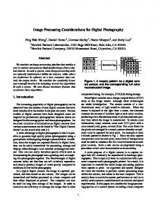
Orig. (top) Detail Transfer (bottom) Flash No-Flash Detail Transfer with Denoising Figure 1: This candlelit setting from the wine cave of a castle is difficult to photograph due to its low light nature. A flash image captures the high-frequency texture and detail, but changes the overall scene appearance to cold and gray. The no-flash image captures the overall appearance of the warm candlelight, but is very noisy. We use the detail information from the flash image to both reduce noise in the no-flash image and sharpen its detail. Note the smooth appearance of the brown leather sofa and crisp detail of the bottles. For full-sized images, please see the supplemental DVD or the project website http://research.microsoft.com/projects/FlashNoFlash.
Abstract Digital photography has made it possible to quickly and easily take a pair of images of low-light environments: one with flash to capture detail and one without flash to capture ambient illumination. We present a variety of applications that analyze and combine the strengths of such flash/no-flash image pairs. Our applications include denoising and detail transfer (to merge the ambient qualities of the no-flash image with the high-frequency flash detail), white-balancing (to change the color tone of the ambient image), continuous flash (to interactively adjust flash intensity), and red-eye removal (to repair artifacts in the flash image). We demonstrate how these applications can synthesize new images that are of higher quality than either of the originals. Keywords: Noise removal, detail transfer, sharpening, image fusion, image processing, bilateral filtering, white balancing, redeye removal, flash photography.
1
Introduction
An important goal of photography is to capture and reproduce the visual richness of a real environment. Lighting is an integral aspect of this visual richness and often sets the mood or atmosphere in the photograph. The subtlest nuances are often found in low-light conditions. For example, the dim, orange hue of a candlelit restaurant can evoke an intimate mood, while the pale blue cast of moonlight can evoke a cool atmosphere of mystery. When capturing the natural ambient illumination in such low-light environments, photographers face a dilemma. One option is to set a long exposure time so that the camera can collect enough light
to produce a visible image. However, camera shake or scene motion during such long exposures will result in motion blur. Another option is to open the aperture to let in more light. However, this approach reduces depth of field and is limited by the size of the lens. The third option is to increase the camera’s gain, which is controlled by the ISO setting. However, when exposure times are short, the camera cannot capture enough light to accurately estimate the color at each pixel, and thus visible image noise increases significantly. Flash photography was invented to circumvent these problems. By adding artificial light to nearby objects in the scene, cameras with flash can use shorter exposure times, smaller apertures, and less sensor gain and still capture enough light to produce relatively sharp, noise-free images. Brighter images have a greater signalto-noise ratio and can therefore resolve detail that would be hidden in the noise in an image acquired under ambient illumination. Moreover, the flash can enhance surface detail by illuminating surfaces with a crisp point light source. Finally, if one desires a white-balanced image, the known flash color greatly simplifies this task. As photographers know, however, the use of flash can also have a negative impact on the lighting characteristics of the environment. Objects near the camera are disproportionately brightened, and the mood evoked by ambient illumination may be destroyed. In addition, the flash may introduce unwanted artifacts such as red eye, harsh shadows, and specularities, none of which are part of the natural scene. Despite these drawbacks, many amateur photographers use flash in low-light environments, and consequently, these snapshots rarely depict the true ambient illumination of such scenes. Today, digital photography makes it fast, easy, and economical to take a pair of images of low-light environments: one with flash to capture detail and one without flash to capture ambient illumination. (We sometimes refer to the no-flash image as the ambient image.) In this paper, we present a variety of techniques that
analyze and combine features from the images in such a flash/noflash pair: Ambient image denoising: We use the relatively noise-free flash image to reduce noise in the no-flash image. By maintaining the natural lighting of the ambient image, our approach creates an image that is closer to the look of the real scene. Flash-to-ambient detail transfer: We transfer high-frequency detail from the flash image to the denoised ambient image, since this detail may not exist in the original ambient image. White balancing: The user may wish to simulate a whiter illuminant while preserving the “feel” of the ambient image. We exploit the known flash color to white-balance the ambient image, rather than relying on traditional single-image heuristics. Continuous flash intensity adjustment: We provide continuous interpolation control between the image pair so that the user can interactively adjust the flash intensity. The user can even extrapolate beyond the original ambient and flash images. Red-eye correction: We perform red-eye detection by considering how the color of the pupil changes between the ambient and flash images. While many of these problems are not new, the primary contribution of our work is to show how to exploit information in the flash/no-flash pair to improve upon previous techniques 1. One feature of our approach is that the manual acquisition of the flash/no-flash pair is relatively straightforward with current consumer digital cameras. We envision that the ability to capture such pairs will eventually move into the camera firmware, thereby making the acquisition process even easier and faster. One recurring theme of recent computer graphics research is the idea of taking multiple photographs of a scene and combining them to synthesize a new image. Examples of this approach include creating high dynamic range images by combining photographs taken at different exposures [Debevec and Malik 1997; Kang et al. 2003], creating mosaics and panoramas by combining photographs taken from different viewpoints [e.g. Szeliski and Shum 1997], and synthetically relighting images by combining images taken under different illumination conditions [Haeberli 1992; Debevec et al. 2000; Masselus et al. 2002; Akers et al. 2003; Agarwala et al. 2004]. Although our techniques involve only two input images, they share the similar goal of synthesizing a new image that is of better quality than any of the input images.
2
Background on Camera Noise
The intuition behind several of our algorithms is that while the illumination from a flash may change the appearance of the scene, it also increases the signal-to-noise ratio (SNR) in the flash image and provides a better estimate of the high-frequency detail. As shown in Figure 2(a), a brighter image signal contains more noise than a darker signal. However, the slope of the curve is less than one, which implies that the signal increases faster than the noise and so the SNR of the brighter image is better. While the flash does not illuminate the scene uniformly, it does significantly increase scene brightness (especially for objects near the camera) and therefore the flash image exhibits a better SNR than the ambient image. As illustrated in Figure 2(b), the improvement in SNR in a flash image is especially pronounced at higher frequencies. Properly exposed image pairs have similar intensities after passing through 1
In concurrent work, Eisemann and Durand [2004] have developed techniques similar to ours for transferring color and detail between the flash/no-flash images.
Figure 2: (a-left) Noise vs. signal for a full-frame Kodak CCD [2001]. Since the slope is less than one, SNR increases at higher signal values. (bright) The digital sensor produces similar log power spectra for the flash and ambient images. However, the noise dominates the signal at a lower frequency in the high-ISO ambient image than in the low-ISO flash image.
the imaging system (which may include aperture, shutter/flash duration, and camera gain). Therefore their log power spectra are roughly the same. However, the noise in the high-ISO ambient image is greater than in the low-ISO flash image because the gain amplifies the noise. Since the power spectrum of most natural images falls off at high frequencies, whereas that of the camera noise remains uniform (i.e. assuming white noise), noise dominates the signal at a much lower frequency in the ambient image than in the flash image.
3
Acquisition
Procedure. We have designed our algorithms to work with images acquired using consumer-grade digital cameras. The main goal of our acquisition procedure is to ensure that the flash/noflash image pair capture exactly the same points in the scene. We fix the focal length and aperture between the two images so that the camera’s focus and depth-of-field remain constant. Our acquisition procedure is as follows: 1. Focus on the subject, then lock the focal length and aperture. 2. Set exposure time Δ𝑡 and ISO for a good exposure. 3. Take the ambient image 𝐴. 4. Turn on the flash. 5. Adjust the exposure time Δ𝑡 and ISO to the smallest settings that still expose the image well. 6. Take the flash image 𝐹. A rule of thumb for handheld camera operation is that exposure times for a single image should be under 1�30s for a 30mm lens to prevent motion blur. In practice, we set the exposure times for both images to 1�60s or less so that under ideal circumstances, both images could be shot one after another within the 1�30s limit on handheld camera operation. Although rapidly switching between flash and non-flash mode is not currently possible on consumergrade cameras, we envision that this capability will eventually be included in camera firmware. Most of the images in this paper were taken with a Canon EOS Digital Rebel. We acquire all images in a RAW format and then convert them into 16-bit TIFF images. By default, the Canon conversion software performs white balancing, gamma correction and other nonlinear tone-mapping operations to produce perceptually pleasing images with good overall contrast. We apply most of our algorithms on these non-linear images in order to preserve their highquality tone-mapping characteristics in our final images. Registration. Image registration is not the focus of our work and we therefore acquired most of our pairs using a tripod setup. Nevertheless we recognize that registration is important for images taken with handheld cameras since changing the camera settings (i.e. turning on the flash, changing the ISO, etc.) often results in camera motion. For the examples shown in Figure 11 we took the photographs without a tripod and then applied the registration technique of Szeliski and Shum [1997] to align them.
Bilateral filter. The bilateral filter is designed to average together pixels that are spatially near one another and have similar intensity values. It combines a classic low-pass filter with an edgestopping function that attenuates the filter kernel weights when the intensity difference between pixels is large. In the notation of Durand and Dorsey [2002], the bilateral filter computes the value of pixel 𝑝 for ambient image 𝐴 as: 𝐴𝐵𝑎𝑠𝑒 = 𝑝
1 � 𝑔𝑑 (𝑝′ − 𝑝) 𝑔𝑟 �𝐴𝑝 − 𝐴𝑝′ � 𝐴𝑝′ , 𝑘(𝑝)
where 𝑘(𝑝) is a normalization term:
𝑘(𝑝) = � 𝑔𝑑 (𝑝′ − 𝑝) 𝑔𝑟 �𝐴𝑝 − 𝐴𝑝′ � .
Figure 3: Overview of our algorithms for denoising, detail transfer, and flash artifact detection.
While we found this technique works well, we note that flash/noflash images do have significant differences due to the change in illumination, and therefore robust techniques for registration of such image pairs deserve further study. Linearization. Some of our algorithms analyze the image difference 𝐹 − 𝐴 to infer the contribution of the flash to the scene lighting. To make this computation meaningful, the images must be in the same linear space. Therefore we sometimes set our conversion software to generate linear TIFF images from the RAW data. Also, we must compensate for the exposure differences between the two images due to ISO settings and exposure times Δ𝑡. If 𝐴′𝐿𝑖𝑛 and 𝐹 𝐿𝑖𝑛 are the linear images output by the converter utility, we put them in the same space by computing: 𝐴𝐿𝑖𝑛 = 𝐴′𝐿𝑖𝑛
ISO𝐹 Δ𝑡𝐹 . ISO𝐴 Δ𝑡𝐴
(1)
Note that unless we include the superscript 𝐿𝐿𝐿, 𝐹 and 𝐴 refer to the non-linear versions of the images.
4
Denoising and Detail Transfer
Our denoising and detail transfer algorithms are designed to enhance the ambient image using information from the flash image. We present these two algorithms in Sections 4.1 and 4.2. Both algorithms assume that the flash image is a good local estimator of the high frequency content in the ambient image. However, this assumption does not hold in shadow and specular regions caused by the flash, and can lead to artifacts. In Section 4.3, we describe how to account for these artifacts. The relationships between the three algorithms are depicted in Figure 3.
4.1
Denoising
Reducing noise in photographic images has been a long-standing problem in image processing and computer vision. One common solution is to apply an edge-preserving smoothing filter to the image such as anisotropic diffusion [Perona and Malik 1990] or bilateral filtering [Tomasi and Manduchi 1998]. The bilateral filter is a fast, non-iterative technique, and has been applied to a variety of problems beyond image denoising, including tone-mapping [Durand and Dorsey 2002; Choudhury and Tumblin 2003], separating illumination from texture [Oh et al. 2001] and mesh smoothing [Fleishman et al. 2003; Jones et al. 2003]. Our ambient image denoising technique also builds on the bilateral filter. We begin with a summary of Tomasi and Manduchi’s basic bilateral filter and then show how to extend their approach to also consider a flash image when denoising an ambient image.
(2)
𝑝′ ∈Ω
𝑝′ ∈Ω
(3)
The function 𝑔𝑑 sets the weight in the spatial domain based on the distance between the pixels, while the edge-stopping function 𝑔𝑟 sets the weight on the range based on intensity differences. Typically, both functions are Gaussians with widths controlled by the standard deviation parameters 𝜎𝑑 and 𝜎𝑟 respectively.
We apply the bilateral filter to each RGB color channel separately with the same standard deviation parameters for all three channels. The challenge is to set 𝜎𝑑 and 𝜎𝑟 so that the noise is averaged away but detail is preserved. In practice, for 6 megapixel images, we set 𝜎𝑑 to cover a pixel neighborhood of between 24 and 48 pixels, and then experimentally adjust 𝜎𝑟 so that it is just above the threshold necessary to smooth the noise. For images with pixel values normalized to [0.0, 1.0] we usually set 𝜎𝑟 to lie between 0.05 and 0.1, or 5 to 10% of the total range. However, as shown in Figure 4(b), even after carefully adjusting the parameters, the basic bilateral filter tends to either over-blur (lose detail) or under-blur (fail to denoise) the image in some regions. Joint bilateral filter. We observed in Section 2 that the flash image contains a much better estimate of the true high-frequency information than the ambient image. Based on this observation, we modify the basic bilateral filter to compute the edge-stopping function 𝑔𝑟 using the flash image 𝐹 instead of 𝐴. We call this technique the joint bilateral filter 2: 𝐴𝑁𝑅 𝑝 =
1 � 𝑔𝑑 (𝑝′ − 𝑝) 𝑔𝑟 �𝐹𝑝 − 𝐹𝑝′ � 𝐴𝑝′ , 𝑘(𝑝)
(4)
𝑝′ ∈Ω
where 𝑘(𝑝) is modified similarly. Here 𝐴𝑁𝑅 is the noise-reduced version of 𝐴. We set 𝜎𝑑 just as we did for the basic bilateral filter. Under the assumption that 𝐹 has little noise, we can set 𝜎𝑟 to be very small and still ensure that the edge-stopping function 𝑔𝑟 �𝐹𝑝 − 𝐹𝑝′ � will choose the proper weights for nearby pixels and therefore will not over-blur or under-blur the ambient image. In practice, we have found that 𝜎𝑟 can be set to 0.1% of the total range of color values. Unlike basic bilateral filtering, we fix 𝜎𝑟 for all images.
The joint bilateral filter relies on the flash image as an estimator of the ambient image. Therefore it can fail in flash shadows and specularities because they only appear in the flash image. At the edges of such regions, the joint bilateral filter may under-blur the ambient image since it will down-weight pixels where the filter straddles these edges. Similarly, inside these regions, it may overblur the ambient image. We solve this problem by first detecting flash shadows and specular regions as described in Section 4.3 and then falling back to basic bilateral filtering within these regions. Given the mask 𝑀 2
Eisemann and Durand [2004] call this the cross bilateral filter.
produced by our detection algorithm, our improved denoising algorithm becomes: ′
𝐴𝑁𝑅 = (1 − 𝑀)𝐴𝑁𝑅 + 𝑀 𝐴𝐵𝑎𝑠𝑒 .
(5)
Results & Discussion. The results of denoising with the joint bilateral filter are shown in Figure 4(c). The difference image with the basic bilateral filter, Figure 4(d), reveals that the joint bilateral filter is better able to preserve detail while reducing noise. One limitation of both bilateral and joint bilateral filtering is that they are nonlinear and therefore a straightforward implementation requires performing the convolution in the spatial domain. This can be very slow for large 𝜎𝑑 .
Recently Durand and Dorsey [2002] used Fourier techniques to greatly accelerate the bilateral filter. We believe their technique is also applicable to the joint bilateral filter and should significantly speed up our denoising algorithm.
Figure 5: (left) A Gaussian low-pass filter blurs across all edges and will therefore create strong peaks and valleys in the detail image that cause halos. (right) The bilateral filter does not smooth across strong edges and thereby reduces halos, while still capturing detail.
4.2
Flash-To-Ambient Detail Transfer
While the joint bilateral filter can reduce noise, it cannot add detail that may be present in the flash image. Yet, as described in Section 2, the higher SNR of the flash image allows it to retain nuances that are overwhelmed by noise in the ambient image. Moreover, the flash typically provides strong directional lighting that can reveal additional surface detail that is not visible in more uniform ambient lighting. The flash may also illuminate detail in regions that are in shadow in the ambient image. To transfer this detail we begin by computing a detail layer from the flash image as the following ratio: 𝐹 𝐷𝑒𝑡𝑎𝑖𝑙 =
(a) No-Flash
Flash
(c) Denoised via Joint Bilateral Filter
(b) Denoised via Bilateral Filter
(d)
Difference
𝐹+𝜀 , 𝐹𝐵𝑎𝑠𝑒 + 𝜀
where 𝐹 𝐵𝑎𝑠𝑒 is computed using the basic bilateral filter on 𝐹. The ratio is computed on each RGB channel separately and is independent of the signal magnitude and surface reflectance. The ratio captures the local detail variation in 𝐹 and is commonly called a quotient image [Shashua and Riklin-Raviv 2001] or ratio image [Liu et al. 2001] in computer vision. Figure 5 shows that the advantage of using the bilateral filter to compute 𝐹 𝐵𝑎𝑠𝑒 rather than a classic low-pass Gaussian filter is that we reduce haloing.
At low signal values, the flash image contains noise that can generate spurious detail. We add 𝜀 to both the numerator and denominator of the ratio to reject these low signal values and thereby reduce such artifacts (and also avoid division by zero). In practice we use 𝜀=0.02 across all our results. To transfer the detail, we simply multiply the noise-reduced ambient image 𝐴𝑁𝑅 by the ratio 𝐹 𝐷𝑒𝑡𝑎𝑖𝑙 . Figure 4(e-f) shows examples of a detail layer and detail transfer.
Just as in joint bilateral filtering, our transfer algorithm produces a poor detail estimate in shadows and specular regions caused by the flash. Therefore, we again rely on the detection algorithm described in Section 4.3 to estimate a mask 𝑀 identifying these regions and compute the final image as: 𝐴𝐹𝑖𝑛𝑎𝑙 = (1 − 𝑀) 𝐴𝑁𝑅 𝐹 𝐷𝑒𝑡𝑎𝑖𝑙 + 𝑀 𝐴𝐵𝑎𝑠𝑒 .
(e)
Detail Layer
(f)
Detail Transfer
Figure 4: (a) A close-up of a flash/no-flash image pair of a Belgian tapestry. The no-flash image is especially noisy in the darker regions and does not show the threads as well as the flash image. (b) Basic bilateral filtering preserves strong edges, but blurs away most of the threads. (c) Joint bilateral filtering smoothes the noise while also retaining more thread detail than the basic bilateral filter. (d) The difference image between the basic and joint bilateral filtered images. (e) We further enhance the ambient image by transferring detail from the flash image. We first compute a detail layer from the flash image, and then (f) combine the detail layer with the image denoised via the joint bilateral filter to produce the detail-transferred image.
(6)
(7)
With this detail transfer approach, we can control the amount of detail transferred by choosing appropriate settings for the bilateral filter parameters 𝜎𝑑 and 𝜎𝑟 used to create 𝐹 𝐵𝑎𝑠𝑒 . As we increase these filter widths, we generate increasingly smoother versions of 𝐹 𝐵𝑎𝑠𝑒 and as a result capture more detail in 𝐹 𝐷𝑒𝑡𝑎𝑖𝑙 . However, with excessive smoothing, the bilateral filter essentially reduces to a Gaussian filter and leads to haloing artifacts in the final image. Results & Discussion. Figures 1, 4(f), and 6–8 show several examples of applying detail transfer with denoising. Both the lamp (Figure 6) and pots (Figure 8) examples show how our detail transfer algorithm can add true detail from the flash image to the ambient image. The candlelit cave (Figure 1 and 7) is an extreme case for our algorithms because the ISO was originally set to 1600 and digitally boosted up to 6400 in a post-processing step. In this
Flash
No-Flash
Orig. (top)
Detail Transfer (bottom)
Flash
No-Flash
Detail Transfer with Denoising
Figure 6: An old European lamp made of hay. The flash image captures detail, but is gray and flat. The no-flash image captures the warm illumination of the lamp, but is noisy and lacks the fine detail of the hay. With detail transfer and denoising we maintain the warm appearance, as well as the sharp detail.
In most cases, our detail transfer algorithm improves the appearance of the ambient image. However, it is important to note that the flash image may contain detail that looks unnatural when transferred to the ambient image. For example, if the light from the flash strikes a surfaces at a shallow angle, the flash image may pick up surface texture (i.e. wood grain, stucco, etc.) as detail. If this texture is not visible in the original ambient image, it may look odd. Similarly if the flash image washes out detail, the ambient image may be over-blurred. Our approach allows the user to control how much detail is transferred over the entire image. Automatically adjusting the amount of local detail transferred is an area for future work.
4.3
No-Flash
Detail Transfer with Denoising
Long Exposure Reference
Figure 7: We captured a long exposure image of the wine cave scene (3.2 seconds at ISO 100) for comparison with our detail transfer with denoising result. We also computed average mean-square error across the 16 bit R, G, B color channels between the no-flash image and the reference (1485.5 MSE) and between our result and the reference (1109.8 MSE). However, it is well known that MSE is not a good measure of perceptual image differences. Visual comparison shows that although our result does not achieve the fidelity of the reference image, it is substantially less noisy than the original no-flash image.
case, the extreme levels of noise forced us to use relatively wide Gaussians for both the domain and range kernels in the joint bilateral filter. Thus, when transferring back the true detail from the flash image, we also used relatively wide Gaussians in computing the detail layer. As a result, it is possible to see small halos around the edges of the bottles. Nevertheless, our approach is able to smooth away the noise while preserving detail like the gentle wrinkles on the sofa and the glazing on the bottles. Figure 7 shows a comparison between a long exposure reference image of the wine cave and our detail transfer with denoising result.
Detecting Flash Shadows and Specularities
Light from the flash can introduce shadows and specularities into the flash image. Within flash shadows, the image may be as dim as the ambient image and therefore suffer from noise. Similarly, within specular reflections, the flash image may be saturated and lose detail. Moreover, the boundaries of both these regions may form high-frequency edges that do not exist in the ambient image. To avoid using information from the flash image in these regions, we first detect the flash shadows and specularities. Flash Shadows. Since a point in a flash shadow is not illuminated by the flash, it should appear exactly as it appears in the ambient image. Ideally, we could linearize 𝐴 and 𝐹 as described in Section 3 and then detect pixels where the luminance of the difference image 𝐹 𝐿𝑖𝑛 − 𝐴𝐿𝑖𝑛 is zero. In practice, this approach is confounded by four issues: 1) surfaces that do not reflect any light (i.e. with zero albedo) are detected as shadows; 2) distant surfaces not reached by the flash are detected as shadows; 3) noise causes nonzero values within shadows; and 4) inter-reflection of light from the flash causes non-zero values within the shadow. The first two issues do not cause a problem since the results are the same in both the ambient and flash images and thus whichever image is chosen will give the same result. To deal with noise and inter-reflection, we add a threshold when computing the shadow mask by looking for pixels in which the difference between the linearized flash and ambient images is small: 𝑀 𝑆ℎ𝑎𝑑 = �
1 when 𝐹 𝐿𝑖𝑛 − 𝐴𝐿𝑖𝑛 ≤ 𝜏𝑆ℎ𝑎𝑑 0 otherwise.
(8)
No-Flash
Flash
Orig. (top)
Detail Transfer (bottom)
Detail Transfer without Mask
Shadow and Specularity Mask
Detail Transfer using Mask
Flash No-Flash Detail Transfer with Denoising Figure 8: (top row) The flash image does not contain true detail information in shadows and specular regions. When we naively apply our denoising and detail transfer algorithms, these regions generate artifacts as indicated by the white arrows. To prevent these artifacts, we revert to basic bilateral filtering within these regions. (bottom row). The dark brown pot on the left is extremely noisy in the no-flash image. The green pot on the right is also noisy, but as shown in the flash image it exhibits true texture detail. Our detail transfer technique smoothes the noise while maintaining the texture. Also note that the flash shadow/specularity detection algorithm properly masks out the large specular highlight on the brown pot and does not transfer that detail to the final image.
We have developed a program that lets users interactively adjust the threshold value 𝜏𝑆ℎ𝑎𝑑 and visually verify that all the flash shadow regions are properly captured.
Noise can contaminate the shadow mask with small speckles, holes and ragged edges. We clean up the shadow mask using image morphological operations to erode the speckles and fill the holes. To produce a conservative estimate that fully covers the shadow region, we then dilate the mask.
Flash Specularities. We detect specular regions caused by the flash using a simple physically motivated heuristic. Specular regions should be bright in 𝐹 𝐿𝑖𝑛 and should therefore saturate the image sensor. Hence, we look for luminance values in the flash image that are greater than 95% of the range of sensor output values. We clean, fill holes, and dilate the specular mask just as we did for the shadow mask. Final Merge. We form our final mask 𝑀 by taking the union of the shadow and specular masks. We then blur the mask to feather its edges and prevent visible seams when the mask is used to combine regions from different images. Results & Discussion. The results in Figures 1 and 6–8 were generated using this flash artifact detection approach. Figure 8 (top row) illustrates how the mask corrects flash shadow artifacts in the detail transfer algorithm. In Figure 1 we show a failure case of our algorithm. It does not capture the striped specular highlight on the center bottle and therefore this highlight is transferred as detail from the flash image to our final result. Although both our shadow and specular detection techniques are based on simple heuristics, we have found that they produce good masks for a variety of examples. More sophisticated techniques developed for shadow and specular detection in single images or stereo pairs [Lee and Bajcsy 1992; Funka-Lea and Bajcsy 1995; Swaminathan et al. 2002] may provide better results and could be adapted for the case of flash/no-flash pairs.
5
White Balancing
Although preserving the original ambient illumination is often desirable, sometimes we may want to see how the scene would appear under a more “white” illuminant. This process is called white-balancing, and has been the subject of much study [Adams et al. 1998]. When only a single ambient image is acquired, the ambient illumination must be estimated based on heuristics or user input. Digital cameras usually provide several white-balance modes for different environments such as sunny outdoors and fluorescent lighting. Most often, pictures are taken with an “auto” mode, wherein the camera analyzes the image and computes an imagewide average to infer ambient color. This is, of course, only a heuristic, and some researchers have considered semantic analysis to determine color cast [Schroeder and Moser 2001]. A flash/no-flash image pair enables a better approach to white balancing. Our work is heavily inspired by that of DiCarlo et al. [2001], who were the first to consider using flash/no-flash pairs for illumination estimation. They infer ambient illumination by performing a discrete search over a set of 103 illuminants to find the one that most closely matches the observed image pair. We simplify this approach by formulating it as a continuous optimization problem that is not limited by this discrete set of illuminants. Thus, our approach requires less setup than theirs. We can think of the flash as adding a point light source of known color to the scene. By setting the camera white-balance mode to “flash” (and assuming a calibrated camera), this flash color should appear as reference white in the acquired images. The difference image Δ = 𝐹 𝐿𝑖𝑛 − 𝐴𝐿𝑖𝑛 corresponds to the illumination due to the flash only, which is proportional to the surface albedo at each pixel 𝑝. Note that the albedo estimate Δ has unknown scale, because both the distance and orientation of the surface are unknown. Here we are assuming either that the surface is diffuse or that its specular color matches its diffuse color. As a
Original No-Flash Estimated ambient illumination White-Balanced Figure 9: (left) The ambient image (after denoising and detail transfer) has an orange cast to it. The insets show the estimated ambient illumination colors 𝐶 and the estimated overall scene ambience. (right) Our white-balancing algorithm shifts the colors and removes the orange coloring .
-0.5
0.0 (No-Flash) 0.33 0.66 1.0 (Flash) Figure 10: An example of continuous flash adjustment. We can extrapolate beyond the original flash/no-flash pair.
counter-example, this is not true of plastics. Similarly, semitransparent surfaces would give erroneous estimates of albedo. Since the surface at pixel 𝑝 has color 𝐴𝑝 in the ambient image and the scaled albedo Δ𝑝 , we can estimate the ambient illumination at the surface with the ratio: 𝐶𝑝 =
𝐴𝑝 , Δ𝑝
(9)
which is computed per color channel. Again, this estimated color 𝐶𝑝 has an unknown scale, so we normalize it at each pixel 𝑝 (see inset Figure 9). Our goal is to analyze 𝐶𝑝 at all image pixels to infer the ambient illumination color 𝑐. To make this inference more robust, we discard pixels for which the estimate has low confidence. We can afford to do this since we only need to derive a single color from millions of pixels. Specifically, we ignore pixels for which either �𝐴𝑝 � < 𝜏1 or the luminance of Δ𝑝 < 𝜏2 in any channel, since these small values make the ratio less reliable. We set both 𝜏1 and 𝜏2 to about 2% of the range of color values.
Finally, we compute the ambient color estimate 𝑐 for the scene as the mean of 𝐶𝑝 for the non-discarded pixels. (An alternative is to select 𝑐 as the principal component of 𝐶, obtained as the eigenvector of 𝐶 𝑇 𝐶 with the largest eigenvalue, and this gives a similar answer.)
Having inferred the scene ambient color 𝑐, we white-balance the image by scaling the color channels as: 1 𝐴𝑊𝐵 𝑝 = 𝐴𝑝 . 𝑐
(10)
Again, the computation is performed per color channel. Results & Discussion. Figure 9 shows an example of white balancing an ambient image. The white balancing significantly changes the overall hue of the image, setting the color of the wood table to a yellowish gray, as it would appear in white light. In inferring ambient color 𝑐, one could also prune outliers and look for spatial relationships in the image 𝐶. In addition, the scene may have multiple regions with different ambient colors, and these could be segmented and processed independently.
1.5
White-balancing is a challenging problem because the perception of “white” depends in part on the adaptation state of the viewer. Moreover, it is unclear when white-balance is desirable. However we believe that our estimation approach using the known information from the flash can be more accurate than techniques based on single-image heuristics.
6
Continuous Flash Adjustment
When taking a flash image, the intensity of the flash can sometimes be too bright, saturating a nearby object, or it can be too dim, leaving mid-distance objects under-exposed. With a flash and non-flash image pair, we can let the user adjust the flash intensity after the picture has been taken. We have explored several ways of interpolating the ambient and flash images. The most effective scheme is to convert the original flash/no-flash pair into YCbCr space and then linearly interpolate them using: 𝐹 𝐴𝑑𝑗𝑢𝑠𝑡𝑒𝑑 = (1 − 𝛼)𝐴 + (𝛼)𝐹 .
(11)
To provide more user control, we allow extrapolation by letting the parameter 𝛼 go outside the normal [0,1] range. However, we only extrapolate the Y channel, and restrict the Cb and Cr channel interpolations to their extrema in the two original images, to prevent excessive distortion of the hue. An example is shown in Figure 10.
7
Red-Eye Correction
Red-eye is a common problem in flash photography and is due to light reflected by a well vascularized retina. Fully automated redeye removal techniques usually assume a single image as input and rely on a variety of heuristic and machine-learning techniques to localize the red eyes [Gaubatz and Ulichney 2002; Patti et al. 1998]. Once the pupil mask has been detected, these techniques darken the pixels within the mask to make the images appear more natural. We have developed a red-eye removal algorithm that considers the change in pupil color between the ambient image (where it is usually very dark) and the flash image (where it may be red). We convert the image pair into YCbCr space to decorrelate luminance
from chrominance and compute a relative redness measure as follows: 𝑅 = 𝐹𝐶𝑟 − 𝐴𝐶𝑟 .
(12)
𝑅 > 𝜏𝐸𝑦𝑒 .
(13)
We then initially segment the image into regions where:
We typically set 𝜏𝐸𝑦𝑒 to 0.05 so that the resulting segmentation defines regions where the flash image is redder than the ambient image and therefore may form potential red eyes. The segmented regions also tend to include a few locations that are highly saturated in the Cr channel of the flash image but are relatively dark in the Y channel of the ambient image. Thus, if 𝜇𝑅 and 𝜎𝑅 denote the mean and standard deviation of the redness 𝑅, we look for seed pixels where: 𝑅 > max[0.6, 𝜇𝑅 + 3𝜎𝑅 ] and 𝐴𝑌 < 𝜏𝐷𝑎𝑟𝑘 .
Flash
Red-Eye Corrected
(14)
We usually set 𝜏𝐷𝑎𝑟𝑘 = 0.6. If no such seed pixels exist, we assume the image does not contain red-eye. Otherwise, we use these seed pixels to look up the corresponding regions in the segmentation and then apply geometric constraints to ensure that the regions are roughly the same size and elliptical. In particular, we compute the area of each region and discard large outliers. We then check that the eccentricity of the region is greater than 0.75. These regions then form a red-eye pupil mask. Finally to correct these red-eye regions we use the technique of Patti et al.[1998]. We first remove the highlights or “glints” in the pupil mask using our flash specularity detection algorithm. We then set the color of each pixel in the mask to the gray value equivalent to 80% of its luminance value. This approach properly darkens the pupil while maintaining the specular highlight which is important for maintaining realism in the corrected output. Results & Discussion. Figure 11 illustrates our red-eye correction algorithm with two examples. The second example shows that our algorithm performs well even when the red-eye is subtle. In both examples our algorithm is able to distinguish the pupils from the reddish skin. Moreover, the specular highlight is preserved and the eye shows no unnatural discoloration. Both of these examples were automatically aligned using the approach of Szeliski and Shum [1997]. Since color noise could invalidate our chromaticity comparison, we assume a relatively noise free ambient image, like the ones generated by our denoising algorithm.
8
No-Flash
Future Work and Conclusions
While we have developed a variety of applications for flash/noflash image pairs, we believe there remain many directions for future work. In some cases, the look of the flash image may be preferable to the ambient image. However, the flash shadows and specularities may be detracting. While we have developed algorithms for detecting these regions, we would like to investigate techniques for removing them from the flash image. Flash shadows often appear at depth discontinuities between surfaces in the scene. Using multiple flash photographs it may be possible to segment foreground from background. Raskar et al. [2003] have recently explored this type of approach to generate non-photorealistic renderings. Motion blur is a common problem for long-exposure images. It may be possible to extend our detail transfer technique to de-blur such images. Recent work by Jia et al. [2004] is beginning to explore this idea.
Closeup with Faint Red-Eye
No-Flash Flash Red-Eye Corrected Figure 11: Examples of red-eye correction using our approach. Although the red eye is subtle in the second example, our algorithm is still able to correct the problem. We used a Nikon CoolPix 995 to acquire these images.
While our approach is designed for consumer-grade cameras, we have not yet considered the joint optimization of our algorithms and the camera hardware design. For example, different illuminants or illuminant locations may allow the photographer to gather more information about the scene. An exciting possibility is to use an infrared flash. While infrared illumination yields incomplete color information, it does provide high-frequency detail, and does so in a less intrusive way than a visible flash. We have demonstrated a set of applications that combine the strengths of flash and no-flash photographs to synthesize new images that are of better quality than either of the originals. The acquisition procedure is straightforward. We therefore believe that flash/no-flash image pairs can contribute to the palette of image enhancement options available to digital photographers. We hope that these techniques will be even more useful as cameras start to capture multiple images every time a photographer takes a picture.
Acknowledgements We wish to thank Marc Levoy for mentoring the early stages of this work and consistently setting an example for scientific rigor. Steve Marschner gave us many pointers on the fine details of digital photography. We thank Chris Bregler and Stan Birchfield for their encouragement and Rico Malvar for his advice. Mike Braun collaborated on an early version of these ideas. Georg would like to thank his parents for maintaining Castle Pyrmont, which provided a beautiful setting for many of the images in the paper. Finally, we thank the anonymous reviewers for their exceptionally detailed feedback and valuable suggestions.
References ADAMS, J., PARULSKI, K. AND SPAULDING, K., 1998. Color processing in digital cameras. IEEE Micro, 18(6), pp. 20-30. AGARWALA, A., DONTCHEVA, M., AGRAWALA, M., DRUCKER, S., COLBURN, A., CURLESS, B., SALESIN, D. H., AND COHEN, M., 2003. Interactive Digital Photomontage. ACM Transaction on Graphics, 23(3), in this volume. AKERS, D., LOSASSO, F., KLINGNER, J., AGRAWALA, M., RICK, J., AND HANRAHAN, P., 2003. Conveying shape and features with image-based relighting. IEEE Visualization 2003, pp. 349-354. CHOUDHURY, P., AND TUMBLIN, J., 2003. The trilateral filter for high contrast images and meshes. In Eurographics Rendering Symposium, pp. 186-196. DEBEVEC, P. E., AND MALIK, J., 1997. Recovering high dynamic range radiance maps from photographs. ACM SIGGRAPH 97, pp. 369-378. DEBEVEC, P., HAWKINS, T., TCHOU, C., DUIKER, H., SAROKIN, W. AND SAGAR, M., 2000. Acquiring the reflectance field of the human face. ACM SIGGRAPH 2000, pp. 145-156. DICARLO, J. M., XIAO, F., AND WANDELL, B. A., 2001. Illuminating illumination. Ninth Color Imaging Conference, pp. 27-34. DURAND, F., AND DORSEY, J., 2002. Fast bilateral filtering for the display of high-dynamic-range images. ACM Transactions on Graphics, 21(3), pp. 257-266. EISEMANN, E., AND DURAND, F., 2004. Flash photography enhancement via intrinsic relighting. ACM Transactions on Graphics, 23(3), in this volume. FLEISHMAN, S., DRORI, I. AND COHEN-OR, D., 2003. Bilateral mesh denoising. ACM Transaction on Graphics, 22(3), pp. 950-953. FUNKA-LEA, G., AND BAJCSY, R., 1995. Active color and geometry for the active, visual recognition of shadows. International Conference on Computer Vision, pp. 203-209. GAUBATZ, M., AND ULICHNEY, R., 2002. Automatic red-eye detection and correction. IEEE International Conference on Image Processing, pp. 804-807. HAEBERLI, P., 1992. Synthetic lighting for photography. Grafica Obscura, http://www.sgi.com/grafica/synth. JIA, J., SUN, J., TANG, C.-K., AND SHUM, H., 2004. Bayesian correction of image intensity with spatial consideration. ECCV 2004, LNCS 3023, pp. 342-354. JONES, T.R., DURAND, F. AND DESBRUN, M., 2003. Non-iterative feature preserving mesh smoothing. ACM Transactions on Graphics, 22(3), pp. 943-949. KANG, S. B., UYTTENDAELE, M., WINDER, S., AND SZELISKI, R., 2003. High dynamic range video. ACM Transactions on Graphics, 22(3), pp. 319-325. KODAK, 2001. CCD Image Sensor Noise Sources. Application Note MPT/PS-0233. LEE, S. W., AND BAJCSY, R., 1992. Detection of specularity using color and multiple views. European Conference on Computer Vision, pp. 99-114.
LIU, Z., SHAN., Y., AND ZHANG, Z., 2001. Expressive expression mapping with ratio images. ACM SIGGRAPH 2001, pp. 271276. MASSELUS, V., DUTRE, P., ANRYS, F., 2002. The free-form light stage. In Eurographics Rendering Symposium, pp. 247-256. OH, B.M., CHEN, M., DORSEY, J. AND DURAND, F., 2001. Imagebased modeling and photo editing. ACM SIGGRAPH 2001, pp. 433-442. PATTI, A., KONSTANTINIDES, K., TRETTER, D. AND LIN, Q., 1998. Automatic digital redeye reduction. IEEE International Conference on Image Processing, pp. 55-59. PERONA, P., AND MALIK, J., 1990. Scale-space and edge detection using anisotropic diffusion. IEEE Transactions on Pattern Analysis and Machine Intelligence, 12(7), pp. 629-639. RASKAR, R., YU, J. AND ILIE, A., 2003. A non-photorealistic camera: Detecting silhouettes with multi-flash. ACM SIGGRAPH 2003 Technical Sketch. SCHROEDER, M., AND MOSER, S., 2001. Automatic color correction based on generic content-based image analysis. Ninth Color Imaging Conference, pp. 41-45. SHASHUA, A., AND RIKLIN-RAVIV, T., 2001. The quotient image: class based re-rendering and recognition with varying illuminations. IEEE Transactions on Pattern Analysis and Machine Intelligence, 23(2), pp. 129-139. SWAMINATHAN, R., KANG, S. B., SZELISKI, R., CRIMINISI, A. AND NAYAR, S. K., 2002. On the motion and appearance of specularities in image sequences. European Conference on Computer Vision, pp. I:508-523 SZELISKI, R., AND SHUM, H., 1997. Creating full view panoramic image mosaics and environment maps. ACM SIGGRAPH 97, pp. 251-258. TOMASI, C., AND MANDUCHI, R., 1998. Bilateral filtering for gray and color images. IEEE International Conference on Computer Vision, pp. 839-846.