digital processing of speech and image signals - Www I6 Informatik ...

Lecture

DIGITAL PROCESSING OF SPEECH AND IMAGE SIGNALS RWTH Aachen, WS 2006/7

Prof. Dr.-Ing. H. Ney, Dr.rer.nat. R. Schl¨ uter Lehrstuhl f¨ ur Informatik 6 RWTH Aachen

1. System Theory and Fourier Transform 2. Discrete Time Systems 3. Spectral Analysis 4. Fourier Transform and Image Processing 5. LPC Analysis 6. Wavelets 7. Coding 8. Image Segmentation and Contour-Finding

Completions: L. Welling, A. Eiden; April 1997 Completions: J. Dahmen, F. Hilger, S. Koepke; Mai 2000 Completions: F. Hilger, D. Keysers; Juli 2001 Translation: M. Popovi´c, R. Schl¨ uter; April 2003 Corrections: D. Stein; October 2006

Literature: • A. V. Oppenheim, R. W. Schafer: Discrete Time Signal Processing, Prentice Hall, Englewood Cliffs, NJ, 1989. • A. Papoulis: Signal Analysis, McGraw-Hill, New York, NY, 1977. • A. Papoulis: The Fourier Integral and its Applications, McGraw-Hill Classic Textbook Reissue Series, McGraw-Hill, New York, NY, 1987. • W. K. Pratt: Digital Image Processing, Wiley & Sons Inc, New York, NY, 1991. Further reading: • T. K. Moon, W. C. Stirling: Mathematical Methods and Algorithms for Signal Processing. Prentice Hall, Upper Saddle River, NJ, 2000. • J. R. Deller, J. G. Proakis, J. H. L. Hansen: Discrete-Time Processing of Speech Signals, Macmillan Publishing Company, New York, NY, 1993. • W. H. Press, S. A. Teukolsky, W. T. Vetterling, B. P. Flannery: Numerical Recipes in C, Cambridge Univ. Press, Cambridge, 1992. • L. Rabiner, B. H. Juang: Fundamentals of Speech Recognition, Prentice Hall, Englewood Cliffs, NJ, 1993. • T. Lehmann, W. Oberschelp, E. Pelikan, R. Repges: Bildverarbeitung f¨ ur die Medizin, Springer Verlag, Berlin, 1997. • L. Berg: Lineare Gleichungssysteme mit Bandstruktur, VEB Deutscher Verlag der Wissenschaften, Berlin, 1986.

Contents 1 System Theory and Fourier Transform 1.1 Introduction . . . . . . . . . . . . . . . 1.2 Linear time-invariant Systems . . . . . 1.3 Fourier Transform . . . . . . . . . . . . 1.4 Properties of the Fourier Transform . . 1.5 Parseval Theorem . . . . . . . . . . . . 1.6 Autocorrelation Function . . . . . . . . 1.7 Existence of the Fourier Transform . . 1.8 δ-Function . . . . . . . . . . . . . . . . 1.9 Motivation for Fourier Series . . . . . . 1.10 Time Duration and Band Width . . . .

. . . . . . . . . .

. . . . . . . . . .

. . . . . . . . . .

. . . . . . . . . .

. . . . . . . . . .

. . . . . . . . . .

. . . . . . . . . .

. . . . . . . . . .

. . . . . . . . . .

. . . . . . . . . .

. . . . . . . . . .

2 Discrete Time Systems 2.1 Motivation and Goal . . . . . . . . . . . . . . . . . . . . . 2.2 Digital Simulation using Discrete Time Systems . . . . . . 2.3 Examples of Discrete Time Systems . . . . . . . . . . . . . 2.4 Sampling Theorem (Nyquist Theorem) and Reconstruction 2.5 Logarithmic Scale and dB . . . . . . . . . . . . . . . . . . 2.6 Quantization . . . . . . . . . . . . . . . . . . . . . . . . . 2.7 Fourier Transform and z–Transform . . . . . . . . . . . . . 2.8 System Representation and Examples . . . . . . . . . . . . 2.9 Discrete Time Signal Fourier Transform Theorem . . . . . 2.10 Discrete Fourier Transform: DFT . . . . . . . . . . . . . . 2.11 DFT as Matrix Operation . . . . . . . . . . . . . . . . . . 2.12 From Continuous Fourier Transform to Matrix Representation of Discrete Fourier Transform . . . . . . . . . . . . . . 2.13 Frequency Resolution and Zero Padding . . . . . . . . . . 2.14 Finite Convolution . . . . . . . . . . . . . . . . . . . . . . 2.15 Fast Fourier Transform (FFT) . . . . . . . . . . . . . . . . 2.16 FFT Implementation . . . . . . . . . . . . . . . . . . . . . i

1 2 11 16 25 33 34 35 36 41 45 51 52 53 56 61 70 72 74 78 88 90 98 102 104 105 108 118

2.17 Cyclic Matrices and Fourier Transform . . . . . . . . . . .

124

3 Spectral analysis 131 3.1 Features for Speech Recognition . . . . . . . . . . . . . . . 132 3.2 Short Time Analysis and Windowing . . . . . . . . . . . . 135 3.3 Autocorrelation Function and Power Spectral Density . . . 159 3.4 Spectrograms . . . . . . . . . . . . . . . . . . . . . . . . . 165 3.5 Filter Bank Analysis . . . . . . . . . . . . . . . . . . . . . 168 3.6 Mel-frequency scale . . . . . . . . . . . . . . . . . . . . . . 171 3.7 Cepstrum . . . . . . . . . . . . . . . . . . . . . . . . . . . 173 3.8 Statistical Interpretation of the Cepstrum Transformation 183 3.9 Energy in acoustic Vector . . . . . . . . . . . . . . . . . . 185 4 Fourier Transform and Image Processing 4.1 Spatial Frequencies and Fourier Transform for Images 4.2 Discrete Fourier Transform for Images . . . . . . . . 4.3 Fourier Transform in Computer Tomography . . . . . 4.4 Fourier Transform and RST Invariance . . . . . . . . 5 LPC Analysis 5.1 Principle of LPC Analysis . . . . . . . . . 5.2 LPC: Covariance Method . . . . . . . . . . 5.3 LPC: Autocorrelation Method . . . . . . . 5.4 LPC: Interpretation in Frequency Domain 5.5 LPC: Generative Model . . . . . . . . . . 5.6 LPC: Alternative Representations . . . . .

. . . . . .

. . . . . .

. . . . . .

. . . . . .

. . . . . .

. . . . . .

. . . . . . . . . .

. . . . . . . . . .

. . . .

187 188 196 197 199

. . . . . .

207 208 212 213 216 221 223

6 Outlook: Wavelet Transform 225 6.1 Motivation: from Fourier to Wavelet Transform . . . . . . 226 6.2 Definition . . . . . . . . . . . . . . . . . . . . . . . . . . . 227 6.3 Discrete Wavelet Transform . . . . . . . . . . . . . . . . . 229 7 Coding (appendix available as separate document)

233

8 Image Segmentation and Contour-Finding

237

ii

List of Figures 1.1

Oscillograms of three time functions composed as sum of 20 partial oscillations. a) φn = 0, b) φn = π2 , c) φn statistical.

3

Amplitude spectrum of a time function composed as sum of 20 partial tones. . . . . . . . . . . . . . . . . . . . . . . . .

3

from left to right: original photo, low-pass and high-pass filtered version . . . . . . . . . . . . . . . . . . . . . . . .

3

Phase manipulation for portion of a speech signal (vowel ’o’) sampled at 8kHz, 25ms analysis window (200 samples), 512 point FFT . . . . . . . . . . . . . . . . . . . . . . . . . . .

4

Phase manipulation for portion of a speech signal (consonant ’n’) sampled at 8kHz, 25ms analysis window (200 samples), 512 point FFT . . . . . . . . . . . . . . . . . . . . . . . .

5

1.6

Phase manipulation for a Heaviside–function (step–function)

6

1.7

Schematic representation of the physiological mechanism of speech production . . . . . . . . . . . . . . . . . . . . . . .

8

2.1

Digital photo . . . . . . . . . . . . . . . . . . . . . . . . .

58

2.2

Gradient image . . . . . . . . . . . . . . . . . . . . . . . .

58

2.3

Several real cases of Laplace Operator subtraction from original image. a) Original image b) Original image minus Laplace Operator (negative values are set to 0 and values above the grey scale are set to the highest grade of grey) .

60

Ideal reconstruction of a band-limited signal (from Oppenheim, Schafer) a) original signal b) sampled signal c) reconstructed signal

64

1.2 1.3 1.4

1.5

2.4

iii

2.5

2.6 2.7 2.8 2.9 2.10 2.11 2.12 2.13

2.14 2.15 2.16 2.17

Sampling of band-limited signal with different sampling rates: b) sampling rate higher than Nyquist rate - exact reconstruction possible c) sampling rate equal to Nyquist rate - exact reconstruction possible d) sampling rate smaller than Nyquist rate - aliasing - exact reconstruction not possible . . . . . . . . . . . . . . . . . . 65 Amplitude spectrum of the voiceless phoneme “s” from the word “ist” . . . . . . . . . . . . . . . . . . . . . . . . . . . 71 Logarithmic amplitude spectrum of the phoneme “s” . . . 71 Amplitude spectrum of the voiced phoneme “ae” from the ¨ . . . . . . . . . . . . . . . . . . . . . . . . . . . word “Ah” 71 Logarithmic amplitude spectrum of the phoneme “ae” . . . 71 Amplitude spectrum of a speech pause . . . . . . . . . . . 71 Logarithmic amplitude spectrum of a speech pause . . . . 71 Hanning window . . . . . . . . . . . . . . . . . . . . . . . 103 Example of a linear convolution of two finite length signals: a) two signals; b) signal x[n-k] for different values of n: i) n < 0, no overlap with h[k], therefore convolution y[n] = 0 ii) n between 0 and Nh + Nx − 2, convolution 6= 0 iii) n > Nh + Nx − 2, no overlap with h[k], convolution y[n] =0 c) resulting convolution y[n]. . . . . . . . . . . . . . . . . . 106 Flow diagram for decomposition of one N -DFT to two N/2– DFTs with N = 8 . . . . . . . . . . . . . . . . . . . . . . . 110 Flow diagram of an 8–point–FFT using Butterfly operations. 111 Flow diagram of an 8–point–FFT using Butterfly operations. 120 Input and output arrays of an FFT. a) The input array contains N (N is power of 2) complex input values in one real array of the length 2N . with alternating real and imaginary parts. b) The output array contains complex Fourier spectrum at N frequency values. Again alternating real and imaginary parts. The array begins with the zero-frequency and then goes up to the highest frequency followed with values for the negative frequencies. . . . . . . . . . . . . . 122 iv

3.1 3.2 3.3 3.4 3.5

Example for the application of the Discrete Fourier Transform (DFT). . . . . . . . . . . . . . . . . . . . . . . . . . .

138

a) signal v[n]; b) DFT-spectrum V [k]; c) Fourier spectrum V (ejω ). . . . . . . . . . . . . . . . . . . . . . . . . . . . . .

146

a) signal v[n]; b) DFT-spectrum V [k]; c) Fourier spectrum V (ejω ). . . . . . . . . . . . . . . . . . . . . . . . . . . . . .

148

a) DFT of length N = 64; b) DFT of length N = 128; c) Fourier spectrum V (ejω ). . . . . . . . . . . . . . . . . . . .

151

Influence of the window function: above: speech signal (vowel “a”); central: 512 point FFT using rectangle window; below: 512 point FFT using Hamming window . . . . . . . . . . . . . . . . . . . . . . . . .

158

3.6

Fourier Transform of a voiced speech segment: a) signal progression, b) high resolution Fourier Transform, c) low resolution Fourier Transform with short Hamming window (50 sampled values), d) low resolution Fourier Transform using autocorrelation function (19 coefficients), e) low resolution Fourier Transform using autocorrelation function (13 coefficients) . . . . . . . . . . . . . . . . . . . . . . . . 162

3.7

Signal progression and autocorrelation function of voiced (left) and unvoiced (right) speech segment . . . . . . . . .

163

Temporal progression of speech signal and four autocorrelation coefficients . . . . . . . . . . . . . . . . . . . . . . . .

164

3.8 3.9

a) wide-band spectrogram: short time window, high time resolution (vertical lines), no frequency resolution; for voiced signals provides information on formant structure b) narrowband spectrogram: long time window, no time resolution, high frequency resolution (horizontal lines); for voiced signals provides information on fundamental frequency (pitch) 166

3.10 Wide-band and narrow-band spectrogram and speech amplitude for the sentence “Every salt breeze comes from the sea”. . . . . . . . . . . . . . . . . . . . . . . . . . . . . . .

167

3.11 Above: logarithmized power spectrum of a spoken vowel (schematic). Below: corresponding cepstrum (inverse Fourier–transform of the logarithmized power spectrum). . . . . . . . . . . .

177

v

3.12 Cepstral smoothing: speech signal (vowel “a”), windowed speech signal (Hamming window), spectrum obtained from the whole cepstrum (blue) and smoothed spectrum obtained from the first 13 cepstral coefficients (red). . . . . . . . . . 3.13 Homomorph analysis of a speech segment: signal progression, homomorph smoothed spectrum using 13 and 19 cepstral coefficients . . . . . . . . . . . . . . . . . . . . . . . .

179

4.1 4.2 4.3 4.4 4.5 4.6

TV–image (analog) . . . . . . Digitized TV–image . . . . . . Amplitude spectrum of Figure Low-pass filtered . . . . . . . High-pass filtered . . . . . . . High-pass enhancement . . . .

193 193 193 193 194 194

5.1

LPC–analysis of one speech segment a) signal progression, b) prediction error (K=12), c) LPC– spectrum with K=12 coefficients, d) spectrum of the prediction error (K=12), e) LPC–spectrum with K=18 coefficients 219 LPC–Spectra for different prediction orders K . . . . . . . 220

5.2

. . . . 4.2 . . . . . .

. . . . . .

. . . . . .

. . . . . .

. . . . . .

. . . . . .

. . . . . .

. . . . . .

. . . . . .

. . . . . .

. . . . . .

. . . . . .

. . . . . .

. . . . . .

. . . . . .

178

List of Tables 2.1 2.2

Fourier transform pairs . . . . . . . . . . . . . . . . . . . . Fourier transform Theorems . . . . . . . . . . . . . . . . .

87 88

Chapter 1 System Theory and Fourier Transform

• Overview: 1.1 Introduction 1.2 Linear time-invariant Systems 1.3 Fourier Transform 1.4 Properties of Fourier Transform 1.5 Parseval Theorem 1.6 Autocorrelation Function 1.7 Existence of the Fourier Transform 1.8 δ–Function 1.9 Fourier Series 1.10 Duration and Band Width

Digital Processing of Speech and Image Signals

1

WS 2006/2007

1.1

Introduction

What distinguishes the Fourier Transform (FT) from other transformations? 1. Mathematical property of linear time-invariant systems: • FT decomposes the time signal into “eigenfunctions” “eigenfunctions” keep their form by passing the linear time-invariant system Ax=λx • Magnitude of FT: shift invariant 2. Physical observation: • Human ear produces sort of FT, essentially only magnitude of FT (strictly speaking: short-time FT) • Example: Time functions with different evolution can sound equally. The human ear either senses sense phase differences of partial tones of the complete sound of stationary processes very weakly, or does not sense them at all. Fourier transform in speech processing: • Calculation of the spectral components of speech • Basic method for obtaining observations (features) for speech recognition


2

WS 2006/2007

φ=0

0

0

φ = π/2

0

0

random φ

0 0

Figure 1.2: Amplitude spectrum of a time function composed as sum of 20 partial tones. 0

Figure 1.1: Oscillograms of three time functions composed as sum of 20 partial oscillations. a) φn = 0, b) φn = π2 , c) φn statistical.

Figure 1.3: from left to right: original photo, low-pass and high-pass filtered version


3

WS 2006/2007

amplitude spectrum

0

original signal

0

0

inverse FT for phase φ(f ) = 0

0

0

Inverse FT for phase φ(f ) =

π 2

0

0

Inverse FT for random phase φ(f )

0

0

Figure 1.4: Phase manipulation for portion of a speech signal (vowel ’o’) sampled at 8kHz, 25ms analysis window (200 samples), 512 point FFT


4

WS 2006/2007

amplitude spectrum

0

original signal

0

0


0

0

inverse FT for phase φ(f ) =

π 2

0

0

inverse FT for random phase φ(f )

0

0

Figure 1.5: Phase manipulation for portion of a speech signal (consonant ’n’) sampled at 8kHz, 25ms analysis window (200 samples), 512 point FFT


5

WS 2006/2007

amplitude spectrum

0

original signal

0


0

0

inverse FT for phase φ(f ) =

π 2

0

0

inverse FT for random phase φ(f )

0

0

Figure 1.6: Phase manipulation for a Heaviside–function (step–function)


6

WS 2006/2007

Why Fourier? Roughly: • Production, description and algorithmic operations on signals (functions or measurement curves over the time axis) can be described very well in Fourier domain (frequency domain). Deeper reason: • Production, description and algorithmic operations on signals are largely based on linear time-invariant (LTI) operations. • Fourier Transform: simple representation of LTI-operations (later: convolution theorem) Why continuous? • Real world is continuous • Computer (digital = time discrete = sampled) model of the real world


7

WS 2006/2007

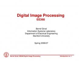
a) A

glottal pulses

vocal tract filter

T

t

b)

speech [a:]

radiation from lips and nose

T

t

|E(f)| [dB]

[a:]

|V(f)| [dB]

|A(f)| [dB]

|S(f)| [dB] [a:]

1/T

0

*

4

=

*

0

4

0

4

0

NOSE OUTPUT NASAL CAVITY

VELUM

PHARYNX CAVITY

VOCAL CORDS

LARYNX TUBE

MOUTH CAVITY TONGUE HUMP

MOUTH OUTPUT

TRACHEA AND BRONCHI

LUNG VOLUME

MUSCLE FORCE

Figure 1.7: Schematic representation of the physiological mechanism of speech production


8

WS 2006/2007

4

signal (speech, image)

feature extraction (signal analysis)

feature vector (pattern vector)

(pattern) comparison

reference data (vectors, features)

decision

Examples: • Spoken language • Written numbers (letters) • Cell recognition (red blood cells)


9

WS 2006/2007

Examples of applications of Fourier Transform: • Electrical switchgears • Recognition and coding – Speech and general acoustic signals – Image signals • Time series analysis: – Astronomical measurement curves – Stock-market course – ... • Computer tomography • Solving differential equations • Description of image production in optical systems


10

WS 2006/2007

1.2

Linear time-invariant Systems

Example: – speech production – electrical systems h(t) input signal x(t)

output signal y(t)

S

symbolic: {t → y(t)} = S {t → x(t)} simplified: y(t) = S {x(t)} • Note: the complete time domain of the function is important, not individual positions in time t. more exact: y = S {x} LTI–System:

(LTI = Linear Time-Invariant)

• Linear: Additive: S {x1 + x2 } = S {x1 } + S {x2 } Homogeneous: S {α x} = αS {x} ,

α ∈ IR

• Time-invariant: {t → y(t − t0 )} = S {t → x(t − t0 )} , Digital Processing of Speech and Image Signals

11

t0 ∈ IR WS 2006/2007

Mathematical theorem: • Linearity and time invariance result in convolution representation • Output signal y(t) of LTI system S with input signal x(t):

y(t) =

=

Z∞

−∞ Z∞

−∞

x(t − τ ) h(τ ) dτ x(τ ) h(t − τ ) dτ

= x(t) ∗ h(t) • h: impulse response of the system S e

(t) ∆τ

x (t)

1/∆τ ∆τ

t

τi

t

• system response h∆τ (t) to excitation e∆τ (t): h∆τ (t) = S {e∆τ (t)} • signal x(t) is represented as sum of amplitude weighted and time shifted elementary functions e∆τ (t): " # X x(t) = lim x(τi ) e∆τ (t − τi ) ∆τ ∆τ →0

i


12

WS 2006/2007

Hence the following holds for the output signal y(t): y(t) = S {x(t)} = S =

(

lim

∆τ →0

"

lim

∆τ →0

S

X

(i

additivity: =

lim

∆τ →0

"

X

x(τi ) e∆τ (t − τi ) ∆τ

X i

)

x(τi ) e∆τ (t − τi ) ∆τ

S { x(τi ) e∆τ (t − τi ) ∆τ }

i

)#

#

homogeneity (for x(τi ) and ∆τ ): " # X = lim x(τi ) S { e∆τ (t − τi ) } ∆τ ∆τ →0

i

time invariance: =

lim

∆τ →0

"

X i

x(τi ) h∆τ (t − τi ) ∆τ

#

limiting case ∆τ → 0 : X

∆τ τi h∆τ (t)

−→ −→ −→ −→

Z

dτ τ h(t)

result: y(t) =

Z∞

−∞

h(t):

x(τ ) h(t − τ ) dτ = x(t) ∗ h(t)

impulse response of the system


13

WS 2006/2007

Examples of LTI-operations: • Oscillatory systems (electrical or mechanical) with external excitation: h(τ )

x(t) −→ y(t) =

Z

−→ y(t)

h(t − τ ) x(τ ) dτ

y ′′ (t) + 2αy ′ (t) + β 2 y(t) = x(t) α, β: parameters depending on the oscillatory system • More general electrical engineering systems: high-pass, low-pass, band-pass

• Sliding average value: x(t) −→

S

−→ y(t) := x(t) +T Z /2

1 x(t) = T

x(t + τ ) dτ

−T /2

• Differentiator: x(t) −→

−→ y(t) := x′ (t)

S

• Comb filter: ”hypothesized” period T x(t) −→

S

−→ y(t) := x(t) − x(t − T )

• In general: linear differential equations with coefficients ck and dl P P ck y (k) (t) = dl x(l) (t) k

l

[ + further constraints ]


14

WS 2006/2007

Example of a non-linear system: system: y(t) = x2 (t) x(t) = A cos(βt) A2 (1 + cos(2βt)) =⇒ y(t) = A cos (βt) = 2 2

2

frequency doubling


15

WS 2006/2007

1.3

Fourier Transform

Sinusoidal oscillation: x(t) = A sin ( ω t + ϕ ) amplitude A phase / null phase ϕ angular frequency ω = 2 π f j 2 = −1,

j∈C

Im 1 sin α α cos α 1

complex representation:

Re

ej α = cos α + j sin α,

ejα + e−jα cos α = 2

and

α ∈ IR

ejα − e−jα sin α = 2j

dimension: DIM(ω) DIM(t) = 1 DIM(ω) =

1 1 = = [Hz] DIM(t) [sec]


16

WS 2006/2007

LTI-System y(t) =

Z∞

−∞

x(t − τ )h(τ )dτ = x(t) ∗ h(t)

• Determine the following specific input signal: x(t) = A ej(ωt+ϕ) • For this input signal the output signal becomes: y(t) =

Z∞

A ej(ω(t−τ )+ϕ) h(τ )dτ

−∞

= A ej(ωt+ϕ)

Z∞

h(τ )e−jωτ dτ

−∞

=

| {z } H(ω) = F {h(τ )} x(t) · H(ω)

• Definition of the Fourier transform: Z∞ h(τ )e−jωτ dτ = F {h(τ )} = F {τ → h(τ )} H(ω) = −∞

(→

decomposition into e−jωτ )

• H(ω) is called transfer function of the system Remark about x(t) = A ej(ωt+ϕ) : • The shape of the input signal x(t), i.e. its frequency ω (“eigenfunction”) remains invariant • Amplitude (intensity) and phase (time shift) are depending on H(ω) (“eigenvalue”) (→

analogy to the problem of eigenvalues in linear algebra)


17

WS 2006/2007

Remarks • FT is complex: H(ω) = Re {H(ω)} + j Im {H(ω)} = |H(ω)| ejΦ(ω) • Amplitude (spectrum):

q Re {H(ω)}2 + Im {H(ω)}2 |H(ω)| =

• Phase (spectrum):  Im {H(ω)}   arctan   Re {H(ω)}         Im {H(ω)}   arctan + π   Re {H(ω)}    Φ(ω) = π    2           π   −     2


18

Re {H(ω)} > 0 Re {H(ω)} < 0 Re {H(ω)} = 0,

Im {H(ω)} > 0

Re {H(ω)} = 0,

Im {H(ω)} < 0

WS 2006/2007

Examples of Fourier transforms: 1. Rectangle function t h(t) = rect( ) = T

H(ω) =

Z∞

1, 0,

|t| ≤ T /2 |t| > T /2

T

−jωt

h(t)e

dt =

−∞

=

Z2

−jωt

e

− T2

i 1 h −jω T jω T2 2 e −e dt = −jω

ωT ) T sin( 2 ωT 2 sin( ) = ωT ω 2 2

(here: Im {H(ω)} = 0) h(t)

t

H(ω)

ω


19

WS 2006/2007

2. Double-sided exponential h(t) = e−α|t|

H(ω) =

=

Z∞

−∞ Z∞

with α > 0

h(t)e−jωt dt

e−(α+jω)t dt +

0

= = = =

Z∞

e−(α−jω)t dt

0

∞ e−(α−jω)t e + −(α + jω) −(α − jω) 0 1 1 0+0− − −(α + jω) −(α − jω) α − jω + α + jω α2 + ω 2 2α α2 + ω 2

−(α+jω)t

• Imaginary part equals 0 • Infinite spectrum • No zeros H(ω )

h(t)

ω

t

• If h(t) is symmetric (i.e. h(t) = h(−t)), imaginary parts drop away and the real part is sufficient Digital Processing of Speech and Image Signals

20

WS 2006/2007

3. Damped oscillations h(t) = e−α|t| cos(βt) with α > 0

H(ω) =

=

Z∞

−∞ Z∞

h(t)e−jωt dt

e−(α+jω)t cos(βt)dt +

0

=

Z∞

=

e−(α−jω)t cos(βt)dt

0

e−(α+jω)t

ejβt + e−jβt dt + 2

0

=

Z∞

Z∞

e−(α−jω)t

ejβt + e−jβt dt 2

0

...

(elementary calculation)

α α + α2 + (ω − β)2 α2 + (ω + β)2

• Limiting case: H(ω)|ω=±β =

1 α + α α2 + (2β)2

=⇒ tends towards ∞ or −∞ if α tends towards 0

H(ω )

h(t)

t


21

|

|

−β

β

ω

WS 2006/2007

4. Modulated rectangle function (“truncated cosine”) cos(β t), |t| ≤ T /2 h(t) = 0, |t| > T /2 H(ω) =

Z∞

h(t)e−jωt dt

−∞ T

=

Z2

cos(β t)e−jωt dt

− T2

=

...

=



(elementary calculation)

T sin (ω − β) T 2   T 2 (ω − β) 2

 T sin (ω + β) 2   +  T (ω + β) 2 h(t)

h(t)

|

|

t

t

H(ω)

H(ω)

ω


22

|

|

−β

β

ω

WS 2006/2007

Fourier Transform pairs (u = ω/2π) Rectangle function

Sinc function

1

1

-1/2

sin(πu) πu

1/2

Squared sinc function

Triangle function

1

1

-1/2

1/2

Exponential function 2α α2+(2πu)2 e-α|x|

Gaussian function e -αx

2

π - πu e α α

2

Unit impulse δ(x)

1


23

WS 2006/2007

Inverse Fourier–transform Z∞

H(ω) =

h(t)e−jωt dt

−∞

1 ˜ h(t) = 2π

assumption:

with:

H(ω) =

=

=

=

H(ω)ejωt dω

−∞

h(τ )e−jωτ dτ

−∞

˜ inserting H(ω) in h(t): ˜ h(t) =

Z∞

Z∞

1 2π

lim

Ω,T →∞



ZΩ

−Ω

1 lim lim 2π Ω→∞ T →∞ 1 π

lim lim

Ω→∞ T →∞

lim

Ω→∞

1 π

Z∞

−∞

= h(t)



ZT



h(τ ) ejω(t−τ ) dτ  dω

−T ZT ZΩ

ejω(t−τ ) dω h(τ ) dτ

−T −Ω ZT

−T

sin (Ω(t − τ )) h(τ ) dτ t−τ

sin (Ω(t − τ )) h(τ ) dτ t−τ

due to: 1 lim Ω→∞ π Z∞

−∞

(→

sin(Ωt) h(t) dt = h(0) t

−∞

formal expression: h(t) =

Z∞ 

1 2π |

Z∞

−∞



ejω(t−τ ) dω  h(τ ) dτ

{z = δ(t − τ )

}

distribution theory, see there for stronger proof)


24

WS 2006/2007

1.4

Properties of the Fourier Transform

Symmetry

H(ω) =

Z∞

h(t) e−jωt dt = F {h(t)}

1 2π

Z∞

−∞

h(t) =

−∞

H(ω) ejωt dω = F −1 {H(ω)}

F 2 {h(t)} = F {H(ω)} = 2πh(−t) F −1 F {h(t)} = F −1 {H(ω)} = h(t) • Time domain and frequency domain are correlated symmetrically. • Properties of FT are valid in both domains, especially the convolution theorem (see later).


25

WS 2006/2007

Theorems for the Fourier transform H(ω) =

Z∞

e−jωt h(t) dt

−∞

consider the equation: H(ω) = F {h(t)} more exact: {ω → H(ω)} = F {t → h(t)} 1. Linearity:

integral operator is linear

2. Inverse scaling, similarity principle: Z∞

h(αt) e−jωt dt =

−∞

F {h(αt)} =

1 |α|

Z∞

ω

h(τ ) e−j α τ dτ

−∞

1 ω H( ), |α| α

α ∈ IR\{0}

Note: Absolute value, because integral boundaries are swapped for α < 0. 3. Shift:

h(t − t0 ) Z∞

−∞

h(t − t0 ) e−jωt dt = e−jωt0 = e−jωt0

Z∞

−∞ Z∞

h(t − t0 ) e−jω(t−t0 ) dt h(τ ) e−jωτ dτ

−∞


26

WS 2006/2007

=⇒ F {h(t − t0 )} = e−jωt0 H(ω) t0 ∈ IR with H(ω) = F {h(t)} important: | F {h(t − t0 )} | = | F {h(t)} |

, because

|e−jωt0 | = |e−ju | = | cos u − j sin u| p cos2 u + sin2 u = = 1 4. Symmetry and antisymmetry: h(t) = h(−t)

results in

h(t) = −h(−t) 5. Complex conjugation: Z∞

Im{H(ω)} = 0

results in

Re{H(ω)} = 0

suppose that h(t) is a complex function

h(t) e−jωt dt

Z∞

=

−∞

−∞ Z∞

=

h(t) ejωt dt

h(t) ejωt dt = H(−ω)

−∞

F {h(t)} = H(−ω) = F {h(t)} Special case:

h(t) is real, so

h(t) = h(t)

=⇒ H(ω) = H(−ω) =⇒ | H(ω) | = | H(−ω) | = | H(−ω) |


27

WS 2006/2007

6. Differentiation: dh dt



∂  1 ∂t 2π

=

1 2π

=

Z∞

Z∞

−∞



H(ω) ejωt dω 

H(ω) jω ejωt dω

−∞

F{

dh(t) } = jω F {h(t)} dt

Interpretation: differentiation = enhancement of high frequencies (due to the multiplication with ω) 7. Integration: F{

Zt

h(τ )dτ } =

−∞

Proof:

1 F {h(t)} jω

similar to differentiation or inversion

8. Modulation principle: F {h(t) cos(ω0 t)} =

Z∞

−∞

h(t) cos(ω0 t) e−jωt dt



Z∞



Z∞

1  h(t) ejω0 t e−jωt dt + h(t) e−jω0 t e−jωt dt  2 −∞  −∞  ∞ Z Z∞ 1  h(t) e−j(ω−ω0 )t dt + h(t) e−j(ω+ω0 )t dt  = 2

=

−∞

=

−∞

1 [ H(ω − ω0 ) + H(ω + ω0 ) ] 2

and similarly F { h(t) sin(ω0 t) } =

1 [ H(ω − ω0 ) − H(ω + ω0 ) ] 2j


28

WS 2006/2007

y(t)

x(t) h(t), H(ω)

Y(ω)

X(ω)

Convolution theorem • Convolution in time domain corresponds to multiplication in frequency domain Z∞ Time domain: y(t) = x(t) ∗ h(t) = x(t − τ ) h(τ ) dτ −∞

Frequency domain: Y (ω) =

=

=

Z∞

−∞ Z∞

−∞ Z∞



e−jωt 

Z∞



h(τ ) x(t − τ ) dτ  dt

 −∞  Z∞ h(τ )  x(t − τ ) e−jωt dt  dτ −∞

h(τ ) X(ω) e−jωτ dτ

−∞

= X(ω)

Z∞

(shifting)

h(τ ) e−jωτ dτ

−∞

= X(ω) H(ω)


29

WS 2006/2007

• Likewise, multiplication in time domain corresponds to convolution in 1 ): frequency domain (note the factor 2π Time domain:

y(t) = a(t) · b(t)

Frequency domain: Y (ω) =

=

Z∞

−∞ Z∞

−∞

=

=

1 2π 1 2π

a(t) · b(t) e−jωt dt 1 a(t) 2π Z∞

−∞ Z∞ −∞

=

Z∞

B(˜ ω )ej ω˜ t e−jωt d˜ ω dt

−∞

B(˜ ω)

Z∞

a(t)e−j(ω−˜ω)t dt d˜ ω

−∞

A(ω − ω ˜ ) · B(˜ ω )d˜ ω

1 A(ω) ∗ B(ω) 2π

• Motivation for the Fourier transform: FT gives the “simplest” representation of the system operation, because every LTI-System can be interpreted as convolution of the input signal x(t) and the impulse response of the system h(t). Convolution can be then efficiently calculated using FT and convolution theorem. • Mathematical: eigenfunctions


30

WS 2006/2007

Example: Oscillator with excitation Oscillator

x(t) −→

−→ y(t)

y ′′ (t) + 2α y ′ (t) + β 2 y(t) = x(t) Z+∞ 1 x(t) = X(ω)ejωt dω 2π y(t) =

y ′ (t) =

y ′′ (t) =

1 2π 1 2π 1 2π

−∞ Z+∞

Y (ω)ejωt dω

−∞ Z+∞

Y (ω)jω ejωt dω

−∞ Z+∞

Y (ω)[−ω 2 ] ejωt dω

−∞

Z+∞ Z+∞ [−ω 2 + 2αjω + β 2 ]Y (ω)ejωt dω = X(ω)ejωt dω

Z+∞

−∞

−∞

−∞

[−ω 2 + 2αjω + β 2 ] Y (ω) − X(ω) ejωt dω = 0 | {z }

∀t

=0

In this way we obtain the transfer function of an oscillator:

H(ω) =

Y (ω) 1 = X(ω) −ω 2 + 2αjω + β 2


31

WS 2006/2007

1 h(t) = 2π

Z+∞ H(ω)ejωt dω

−∞

(can be given explicitly)

Z+∞ x(t) h(t − τ )dτ y(t) = −∞

Note: y(t) does not contain the component which corresponds to the homogeneous differential equation of the oscillator.

x(t)

Convolution with h(t)

Inverse Fourier Transform

Fourier Transform

X(ω)

y(t)

Multiplication with H(ω) = F{h(t)}


32

Y(ω)

WS 2006/2007

1.5

Parseval Theorem

Convolution theorem: F −1 {H(ω) X(ω)} = (⋆)

1 2π

Z∞

H(ω) X(ω) ejωτ dω

−∞

Z∞

−∞

h(t) x(τ − t) dt

= (h ∗ x) (τ )

We make two special assumptions: i) x(−t) := h(t), then: X(ω) = H(ω) ii) τ = 0 Inserting in (⋆) results in: 1 2π

Z∞

−∞

1 2π

H(ω)H(ω) dω Z∞

−∞

Z∞

=

|H(ω)|2 dω

=

−∞ Z∞

−∞

h(t)h(t) dt

|h(t)|2 dt = E

• Energy E in time domain = Energy E in frequency domain 1 1 ; aid: use normalization factor √ for both (up to the factor 2π 2π directions of Fourier Transform) • Physical aspect: energy conservation • Mathematical aspect: unitary (orthogonal) representation in vector space • |H(ω)|2 is called power spectral density.


33

WS 2006/2007

1.6

Autocorrelation Function

Autocorrelation function • Autocorrelation function of time continuous signal or function h(t) is defined as: R(t) =

Z∞

h(τ ) h(t + τ )dτ

−∞

• The following equation is valid: R(t) = h(t) ∗ h(−t)

→

• Fourier transform gives:

which results in

R(t) = R(−t)

(”Wiener-Khinchin Theorem”)

F {R(t)} = H(ω) H(ω) = |H(ω)|2 • Thus: Fourier transform connects autocorrelation function R(t) and power spectral density |H(ω)|2 |H(ω)|2 =

Z∞

R(t) e−jωt dt =

Z∞

R(t) cos(ωt) dt

−∞

−∞

• Remark: autocorrelation is a special case of the cross correlation between signals x(τ ) and h(t)

Ch,x =

Z∞

h(τ ) x(t + τ )dτ

−∞


34

WS 2006/2007

1.7

Existence of the Fourier Transform

Conditions for h(t) for the existence of the Fourier transform

H(ω) =

Z∞

1 h(t) = 2π

e−jωt h(t) dt ,

−∞

Z∞

ejωt H(ω) dω

−∞

When are those equations valid? Sufficient conditions: 1. h(t) is absolutely integrable: Z∞

−∞

|h(t)|dt < ∞

2. h(t) has finite number of jumps, minima and maxima in each interval of IR 3. h(t) has no infinite jumps More general conditions are possible (but rather complex set of conditions): • Generalized functions, distributions, definition as functional • Example: δ-function: Z∞

δ(t) h(t) dt = h(0) for all functions h

−∞


35

WS 2006/2007

Impulse response: y(t) =

Z∞

−∞

h(t − τ )δ(τ ) dτ

= h(t) ∗ δ(t) = h(t) Consequence: h(t) ≡ 1 ⇒

Z∞

δ(t) dt = 1

−∞

• A function like δ(t) does not “exist”. But it is possible to define the functional for each function t → h(t): ˜ [t → h(t)] −→ δ(h) := h(0)

1.8

δ-Function

Starting point: definition of the δ-function as a boundary case of a function δǫ (t): lim

Z+∞

ǫ→0 −∞

f (t) δǫ (t) dt = f (0)

(1.1)

• Possible realizations of δǫ (t)   1 t ∈ [−ǫ, +ǫ] 2ǫ a) δǫ (t) =  0 otherwise b) δǫ (t) =

1 ǫ π ǫ2 + t2


36

WS 2006/2007

c) δǫ (t) =

1 sin (t/ǫ) π t

d) δǫ (t) = √

1 2πǫ2

t2 − e 2ǫ2

• During inversion of the Fourier transform we have “formally” obtained: δ(t) =

1 2π

Z+∞

ejωt dω = lim

Ω→∞

1 sin (Ωt) π t

(1.2)

−∞

Fourier transform F {δ(t)}: F {δ(t)} =

Z+∞

e−jωt δ(t) dt

−∞

due to (1.1) the following holds: F {δ(t)} = ejωt |t=0 = 1 • Another derivation using (1.2): δ(t) =

=

1 2π 1 2π

Z+∞

−∞ Z+∞

ejωt F {δ(t)} dω ejωt dω

general

according to (1.2)

−∞

Comparison results in: F {δ(t)} = 1


37

WS 2006/2007

From this we obtain the following equations: From symmetry property: F {1} = 2 π δ(ω) From shifting theorem: F {ejω0 t 1} = 2 π δ(ω − ω0 )

cos (ω0 t) = =

1 jω0 t e + e−jω0 t 2   Z+∞ Z+∞ 1  δ(ω + ω0 ) ejωt dω  δ(ω − ω0 ) ejωt dω + 2

= π

−∞ Z+∞

1 2π

−∞

−∞

[ δ(ω − ω0 ) + δ(ω + ω0 ) ] ejωt dω

F { cos (ω0 t) } = π [ δ(ω − ω0 ) + δ(ω + ω0 ) ] Note: another derivation: consider “damped oscillations” 1 −α|t| e cos (ω0 t) 2π in the limit α → 0 .


38

WS 2006/2007

Comb function • define “comb function” (pulse train, sequence of δ-impulses): +∞ X

x(t) =

n=−∞

δ(t − nT )

• Fourier transform of comb function: X(ω) =

Z+∞

x(t) e−jωt dt

−∞

=

=

=

Z+∞ X +∞

δ(t − nT ) e−jωt dt

X

δ(t − nT ) e−jωt dt

−∞ n=−∞ +∞ +∞ Z

n=−∞−∞ +∞ X −jωnT

e

n=−∞

= =

...

(see Papoulis 1962, p. 44)

+∞ 2π X 2π δ(ω − n ) T n=−∞ T

• in words: δ-impulse sequence with period T in time domain produces δ-impulse sequence with period T1 in frequency domain (i.e. 2π T in ω-frequency domain) comb function is transformed to comb function Digital Processing of Speech and Image Signals

39

WS 2006/2007

Comb function

Σ

n=-

-6T

2π T

δ(t-nT)

-3T -T

T

3T

Σ

n=-

-6π -4π -2π T T T

6T

δ(ω-n2π/T)

2π 4π 6π T T T

1(δ(ω-ω )+δ(ω+ω )) 0 0 2

cos(ω0t)

−ω0

ω0

1 j(−δ(ω-ω )+δ(ω+ω )) 0 0 2

sin(ω0t)

ω0 −ω0


40

WS 2006/2007

1.9

Motivation for Fourier Series x:

IR −→ IR t −→ x(t)

Consider a periodical function x with period T : x(t) = x(t + T ) then also x(t) = x(t + kT )

for each t ∈ IR for k ∈ Z

Examples: • Constant function: x0 (t) = A0 • Harmonic oscillator: x1 (t) = A1 cos (

2π t + ϕ1 ) , T

A1 > 0

• All higher harmonic: xn (t) = An cos (n

2π t + ϕn ) , T

An > 0

therefore x(t) =

∞ X

An cos (n ω0 t + ϕn ) with ω0 =

n=0

is periodical with period T =

2π , T

An ≥ 0

2π ω0

• Another notation: x(t) =

∞ X

Bn e−j n ω0 t

where Bn

is a complex number

n=−∞


41

WS 2006/2007

Line spectrum representation

Real measured signal has always a ”widespread” spectrum. Reasons: • Strictly periodical signal (almost) never exists – Period can fluctuate – ”Wave form” within one period can fluctuate – Only a finite section of the signal is analyzed (”window function”) • Only a strictly periodical signal has a sharp line spectrum Remarks: • Fourier series are actually not strictly related to periodical functions: a finite interval of IR is sufficient (the signal is then interpreted as infinitely prolonged). • By transition from the finite interval to the complete real axis the Fourier series becomes Fourier integral.


42

WS 2006/2007

Calculation of Fourier coefficients: • Consider a periodical function x(t) with period T =

2π ω0

• approach: x(t) =

+∞ X

an ej n ω0 t

a∈C

n=−∞

• multiplication with e−j m ω0 t where m ∈ IN and integration over one period result in: +T Z /2

x(t) e−j m ω0 t dt =

+∞ X

ej (n−m) ω0 t dt

an

n=−∞

−T /2

+T Z /2

−T /2

• Due to “orthogonality” holds: +T Z /2

j (n−m) ω0 t

e

dt =

−T /2

T 0

if n = m if n = 6 m

• Then: ZT /2

x(t) e−j m ω0 t dt = am T

−T /2

• Result: an

=

1 T

+T Z /2

x(t) e−j n ω0 t dt

−T /2

=

1 T

+T Z /2

x(t) cos (n ω0 t) dt − j

−T /2

1 T

+T Z /2

x(t) sin (n ω0 t) dt

−T /2


43

WS 2006/2007

Spectrum of a periodical function • If x(t) is periodical with the period T =

x(t) =

+∞ X

2π ω0

an ej n ω0 t ,

n=−∞

, then

an ∈ C

• The Fourier transform X(ω) is: X(ω) = F {x(t)} +∞ X an = n=−∞

+∞ X

= 2π

F {ej n ω0 t } | {z } = 2πδ(ω − nω0 )

n=−∞

an δ(ω − nω0 )

• Note:

This derivation is formal, because the Fourier integral does not exist in the “usual sense”; strict derivation within the scope of distribution theory.

• In words:

a periodic function with the period T has a Fourier transform in the form of a line spectrum with the distance ω0 = 2π T between the components.


44

WS 2006/2007

1.10

Time Duration and Band Width

1. Similarity principle: F {h(αt)} =

1 ω H( ) |α| α

h(t)

H( ω )

ω

t

0 2ωΒ b)

...

... −ωΒ

-ΩS

ΩS

ωΒ

ω

XS2(ω) , ΩS = 2ωΒ (Nyquist rate) c)

...

... -ΩS

−ωΒ

ωΒ

ΩS

ω

XS3(ω) , ΩS < 2ωΒ (aliasing) d)

...

... ωΒ ΩS

Β −Ω−ω S

ω

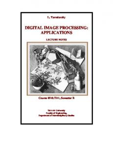
Figure 2.5: Sampling of band-limited signal with different sampling rates: b) sampling rate higher than Nyquist rate - exact reconstruction possible c) sampling rate equal to Nyquist rate - exact reconstruction possible d) sampling rate smaller than Nyquist rate - aliasing - exact reconstruction not possible


65

WS 2006/2007

Another proof using delta- and comb-function: Sampling of the continuous signal x(t) with ΩS =

2π TS

• Band limitation: X(ω) = 0 for |ω| ≥ ωB

(always possible: analog to low-pass with T (ω) = 0 for |ω| ≥ ωB )

• Sampling procedure

Multiplication of a function with a comb-function in time domain

xs (t) = Ts x(t) ·

+∞ X

n=−∞

δ(t − nTs )

results in a convolution with a comb-function in frequency domain: +∞ 1 2πn 2π X Xs (ω) = Ts · X(ω) ∗ δ ω−ω ˜ 2π Ts n=−∞ Ts Z+∞ +∞ X 2πn d˜ ω δ ω−ω ˜ X(˜ ω) = T s n=−∞ −∞ +∞ X

2π X ω−n = Ts n=−∞

=⇒ sampled signal has periodical Fourier spectrum (Analogy to Fourier series: periodical signal has line spectrum, i.e. discrete spectrum) No overlap if:

ωB ≤ ΩS − ωB 2ωB ≤ ΩS Digital Processing of Speech and Image Signals

66

WS 2006/2007

• In so-called digital simulation, the signal x(t) is represented by its sampled values x(n · TS ) measured at equidistant time points with distance TS . With a proper sampling period TS an exact reconstruction of the signal x(t) from the sampled values x(n · TS ) is possible. • If it is possible to exactly reconstruct the signal x(t) from the sampled values x(n·TS ), then it is possible to perform a discrete time processing of the sampled values x(n · TS ) on a computer, which is equivalent to the continuous time processing of the signal x(t) (digital simulation). • Continuous time processing: y(t) =

Z∞

−∞

x(τ ) h(t − τ ) dτ

• Discrete time processing: – Sampling period TS – x[n] := x(nTS ) y(nTS ) = y[n] =

∞ X

k=−∞ ∞ X

k=−∞

x(kTS ) h(nTS − kTS ) TS ,

˜ h[n] = h(nTS )

˜ − k] x[k] h[n

• As a result of the convolution theorem (convolution in time domain corresponds to multiplication in frequency domain), the band limited input signal gives an also band limited output signal which is exactly determined by its sampled values.


67

WS 2006/2007

Important: • In the domain |ω| < ΩS /2 the Fourier transform of a continuous time signal x(t) is identical with the Fourier–transform of the corresponding sampled discrete time signal x(nTS ): Z∞

X(ω) =

x(t) exp(−jωt) dt

−∞

for |ω| ≤ ΩS /2 is identical to ∞ X x(nTS ) exp(−jωTS n) TS · XS (ω) = TS · = TS ·

n=−∞ ∞ X

x(nTS ) exp(−j

n=−∞

2πω n) ΩS

• Inverse Fourier transform of discrete time signal: x(nTS ) =

1 ΩS

Ω ZS /2

XS (ω) exp(jωTS n) dω

−ΩS /2

• One period: ΩS ΩS ≤ ω ≤ 2 2 2πω ≤ π −π ≤ ΩS

−

• The Fourier transform of a discrete time signal is periodic in ω with the period 2 π/TS = ΩS . • The Fourier transform of a discrete time signal is continuous in ω.


68

WS 2006/2007

Frequency normalization • Define the normalized frequency ωN : ωN : = 2π • Definition:

ω ΩS

(ω now denotes a normalized frequency)

– Fourier transform of discrete time signal x[n]: +∞ X

jω

X(e ) =

x[n] exp(−jωn)

n=−∞

Note the notation X(ejω ). – Inverse Fourier transform of discrete time signal x[n]: 1 x[n] = 2π

Zπ

X(ejω ) exp(jωn) dω

−π


69

WS 2006/2007

2.5

Logarithmic Scale and dB

Why? – large dynamic range for the amplitude values of a signal x(t) = A cos βt A :=

amplitude (pressure, velocity, inclination, current, voltage, ... ) “linear” variable

A0 :=

reference amplitude predefined value for calibration

dB := “decibel”

A[dB] ≡ 20 · lg

A , A0

A2 = 10 · lg 2 , A0

lg ≡ log10 A2 = quadratic variable = energy, intensity

because of 210 = 1024 ∼ = 103 : 1 bit more = ˆ

factor 2 for amplitude = ˆ 6 dB = factor 4 for intensity

3 dB = ˆ factor 2 for intensity


70

WS 2006/2007

Phonem: s

Phonem: s

7

2

6

1.5 1

5

0.5 A

log A

4 3

0 -0.5

2

-1

1 0

-1.5 0

1000

2000

3000

4000 f / Hz

5000

6000

7000

-2

8000

Figure 2.6: Amplitude spectrum of the voiceless phoneme “s” from the word “ist”

0

1000

2000

3000

4000 f / Hz

5000

6000

7000

8000

Figure 2.7: Logarithmic amplitude spectrum of the phoneme “s”

Phonem: ae

Phonem: ae

12

2.5 2

10

1.5 1 log A

A

8

6

0.5 0

4

-0.5 2

0

-1 0

1000

2000

3000

4000 f / Hz

5000

6000

7000

-1.5

8000

Figure 2.8: Amplitude spectrum of the voiced phoneme “ae” from the word ¨ “Ah”

0

1000

2000

3000

4000 f / Hz

5000

6000

7000

8000

Figure 2.9: Logarithmic amplitude spectrum of the phoneme “ae”

Pause

Pause

1

0

0.9 -0.5

0.8 0.7

-1 log A

A

0.6 0.5

-1.5

0.4 -2

0.3 0.2

-2.5

0.1 0

0

1000

2000

3000

4000 f / Hz

5000

6000

7000

-3

8000

Figure 2.10: Amplitude spectrum of a speech pause

0

1000

2000

3000

4000 f / Hz

5000

6000

7000

8000

Figure 2.11: Logarithmic amplitude spectrum of a speech pause


71

WS 2006/2007

2.6

Quantization

• Uniform quantization

-X MAX

XMAX

• Quantisation: xˆ = Q(x) • B bits correspond to 2B quantisation levels • Boundaries:

x0 , x1 , . . . , xk , . . . , xK

where

K = 2B

• Width △ of one quantisation level using uniform quantisation: △ =

2 · XM AX 2B

• Quantisation error: σe2

Z+∞ Zxk K X = (x − xˆ)2 p(x) dx = (x − xˆk )2 p(x) dx k=1 x k−1

−∞

– for uniform quantisation: a) b)

xk − xk−1 = △ = const(k) xˆk = 12 (xk−1 + xk )

– uniform distribution with p(x) = const(x) results in:

σe2

=

X △2 k

2 1 △2 XM AX · = = 12 K 12 3 · 22B


72

WS 2006/2007

• signal-to-noise ratio in dB (general definition): σx2 SN R[dB] := 10 lg 2 σn σx2 = power of the signal x σn2 = power of the noise n SN R = signal-to-noise ratio • signal-to-quantisation noise ratio (special case): σx2 SN R[dB] := 10 lg 2 σe σe2 = power of the noise caused by quantisation errors • uniform quantisation using B bits: SN R[dB] = 6.02 B + 4.77 − 20 lg

XM AX σx

• if signal amplitude has Gaussian distribution, only 0.064% of samples have amplitude greater than 4σx : SN R[dB] = 6.02 B − 7.2


73

for XM AX = 4σx

WS 2006/2007

2.7

Fourier Transform and z–Transform

Transfer function and Fourier transform Eigenfunctions of discrete linear time invariant systems (analog to time continuous case): x[n] = ej ω n

−∞ < n < ∞

(ω is dimensionless here) Proof: x[n] = ej ω n ∞ X y[n] = h[k] ej ω (n−k) k=−∞

∞ X

jωn

= e

h[k] e−j ω k

k=−∞

Define:

H(ej ω ) =

∞ P

h[k] e−j ω k

k=−∞

Remark: The Fourier transform of a discrete time signal is already introduced as Fourier series during the derivation of sampling theorem and reconstruction formula (equation (2.2)). Result:

y[n] = ej ω n H(ej ω )


74

WS 2006/2007

z–transform: • Fourier transform of a discrete time signal: x[n] +∞ X

jω

X(e ) =

x[n] e−jωn

n=−∞

–

periodic in ω

–

ω is normalized frequency, thence: −π < ω ≤ π

–

X is evaluated on the unit circle (ejω )

• Generalization: X is evaluated for any complex values z. • That results in z–transform:

+∞ X

X(z) =

x[n] z −n

n=−∞

• Reasons for z–transform 1. analytically simpler, function theory methods are applicable 2. better handling of convergence problem: – convergence of finite signal, i.e. x[n] = 0 for each n > N0 – convergence of infinite signal depends on z • Inverse z–transform:

I

1 x[n] = 2πj

formally: z = ejω

X(z) z n−1 dz

dz = jzdω x[n] =

1 2π

Z2π

X(ejω ) ejωn dω

0


75

WS 2006/2007

Example of Fourier transform and z–transform: • “Truncated geometric series” n a x[n] = 0 • z–transform

N −1 X

X(z) =

n

a z

−n

0≤n≤N −1 otherwise

=

n=0

1

=

z N −1

N −1 X

−1 n

(a z )

n=0

N

N

z −a z−a

1 − (a z −1 )N = 1 − a z −1

• Fourier transform z–transform results in Fourier transformation using substitution

z = ejω

jω

X(e ) =

1 − aN e−jωN 1 − a e−jω special case for a = 1 (discrete time rectangle):

ωN sin ω(N − 1) 2 ω = exp −j 2 sin 2


76

WS 2006/2007

Proof for the z–transform inversion • Statement:

1 x[k] = 2πj

I

X(z) z k−1 dz

• Cauchy integration rule I 1 1 k=1 z −k dz = 0 k 6= 1 2πj I I X 1 1 x[n] z −n+k−1 dz X(z) z k−1 dz = 2πj 2πj n I X 1 x[n] = z −n+k−1 dz 2πj n | {z } 6= 0 only for n = k = x[k]

• Fourier: z = ejω

=⇒

dz = j ejω dω

Then: x[n] =

1 2πj

Z+π

X(ejω ) (ejω )n−1 j ejω dω

−π

Integration path is unit circle because of ejω

=

1 2π

Z+π

X(ejω ) ejωn dω

−π


77

WS 2006/2007

2.8

System Representation and Examples

Example 1: Difference calculation • Difference equation y[n] = x[n] − x[n − n0 ], • Fourier transform gives: ∞ X

−jωn

y[n] e

n=−∞

=

∞ X

n0 integral number

−jωn

x[n] e

n=−∞

Y (ejω ) = X(ejω ) − jω

∞ X

n=−∞ −jωn0

= X(e ) − e • Then follows:

−

∞ X

n=−∞

x[n − n0 ] e−jωn

x[n] e−jωn e−jωn0 X(ejω )

Y (ejω ) H(e ) = X(ejω ) = 1 − e−jωn0 jω

|H(ejω )|2

= (1 − cos(ωn0 ))2 + sin2 (ωn0 ) = 1 − 2cos(ωn0 ) + cos2 (ωn0 ) + sin2 (ωn0 ) = 2 (1 − cos(ωn0 ))

|H(eiω )|2 5

4

3

2

1

0

ω Digital Processing of Speech and Image Signals

78

π n0

WS 2006/2007

Example 2: First order difference equation x[n] y[n] +

α

Delay y[n-1]

x[n] + α y[n − 1] = y[n] y[n] − α y[n − 1] = x[n]

⇐⇒

Method 1: Estimation of transfer function H(ejω ) from impulse response h[n]: • From the Eq. above with y[n] = h[n] and x[n] = δ[n] follows: h[n] = δ[n] + α h[n − 1] = δ[n] + α δ[n − 1] + α2 δ[n − 2] + · · · n α , n≥0 = 0, otherwise • Fourier spectrum/transfer function H(ejω ) jω

H(e ) = = =

+∞ X

h[k] e−jωk

k=−∞ +∞ X

αk e−jωk

k=0 +∞ X

α e−jω

k=0

=

1 1 − α e−jω


79

k

for |α| < 1 WS 2006/2007

Method 2: Estimation of transfer function H(ejω ) using Fourier transform of difference equation: • Difference equation: y[n] − α y[n − 1] = x[n] • Fourier–transform: Y (ejω ) − α e−jω Y (ejω ) = X(ejω ) • Result: H(ejω ) = =


80

Y (ejω ) X(ejω ) 1 1 − α e−jω

WS 2006/2007

Example 3: Linear difference equations (with constant coefficients) • Difference equation: y[n] =

I X i=0

b[i] x[n − i] −

• z-transform: Y (z) = X(z)

I X

b[i]z

−i

i=0

• Result: H(z) =

=

Y (z) X(z) I P

J X

a[j]z −j

j=1

b[i] z −i

1+

j=1

=

j=1

a[j] y[n − j]

− Y (z)

i=0 J P

+∞ X

J X

a[j] z −j

h[n] z −n

n=−∞

Using the definition of H(z) we can optain the impulse response as a function of the coefficients of the difference equation in the above term. Remark: If we factorise denominator and numerator polynoms into linear factors, we can obtain a zero-pole-representation of a discrete time LTI system: ΠI (z − vi ) H(i) = Ji=1 Πj=1 (z − wj ) with zeros vi ∈ C and poles wj ∈ C. Digital Processing of Speech and Image Signals

81

WS 2006/2007

• in general: h[n] has infinite number of non-zero values =⇒ IIR–filter: Infinite Impulse Response

• but if: a[j] ≡ 0 ∀j h[n] identical to zero outside of a finite interval

h[n] =

b[n] 0

n = 0, . . . , I otherwise

=⇒ FIR–filter: Finite Impulse Response


82

WS 2006/2007

Example 4: Impulse response as “truncated geometric series” h[n] =

H(z) =

an 0 M X

0≤n≤M otherwise

n

a z

−n

n=0

a ∈ IR

1 − aM +1 z −(M +1) = 1 − a z −1

system operation:

y[n] =

∞ X

k=−∞

=

M X

k=0

h[k] x[n − k]

ak x[n − k]

or as difference equation (“recursively”) y[n] − a y[n − 1] = x[n] − aM +1 x[n − M − 1]


83

WS 2006/2007

For this example we consider the zero-pole-representation: 1 − ( az )−(M +1) H(z) = 1 − ( az )−1 Zeros: Pole:

zk z0

α>0

2πk

k = 0, 1, . . . , M = a · ej M +1 = a (cancelled by zero z0 = a)

Im M=11

a

Re


84

WS 2006/2007

Example 5: Fibonacci numbers Difference equation: n≥0

h[n + 2] = h[n + 1] + h[n] h[0] = h[1] = 1 h[n] = 0

n>= 1; } j += m; } Here begins the Danielson-Lanczos section of the routine. mmax=2; while (n > mmax) { Outer loop executed log2 nn times istep=mmax 0. We consider the family of window functions Wab (t): t−b wab (t) := w a Digital Processing of Speech and Image Signals

226

WS 2006/2007

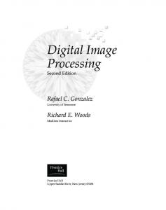
6.2

Definition

The following notation is usually used for the Wavelet–transform: t−b 1 ψab (t) := √ · ψ a a

which is the so-called Mother-Wavelet t → ψ(t).

Like the window function for the short–time Fourier transform the MotherWavelet should be “localized” as much as possible. Example: Mexican-Hat Function:

1 2

ψ(t) = (1 − t2 )e− 2 t

ψ (t)

t


227

WS 2006/2007

The wavelet–transform of f (t) with respect to ψ(t) is defined as: 1 Fψ (a, b) = a

Z+∞

−∞

t−b f (t) · ψ dt a

with scaling parameter a > 0 and localization parameter b ∈ IR. For the inverse transformation holds: Z+∞ Z+∞ t−b 1 1 f (t) = · · da db Fψ (a, b) · ψ Cψ a2 a −∞

0

with Cψ :=

Z∞ 0

|ψ(ω)|2 dω < ∞ ω

Proof (principle only): The proof uses the (generalized) Parseval Theorem:

Fψ (a, b)

1 = √ a 1 = √ a

with

Z+∞

−∞ Z+∞ −∞

1 ψab (t) = √ · ψ a

f (t) · ψ ab (t) dt F (ω) · ψab (ω) dω

t−b a

using further conversions.


228

WS 2006/2007

6.3

Discrete Wavelet Transform

For the scaling parameters a > 0 we choose: a = α0m

where α0 > 1 and m ∈ Z.

The values of m determine the width of wavelet ψab (t).

In order to adjust the localization parameter properly, we define: b = n b0 am 0

where b0 > 0 and n ∈ Z.

Thus we constrain the Wavelet transform to discrete values: Fψ (a, b)

→

Fψ (n, m)

The choice of the function ψ(t) is still open. It is useful to choose ψ(t) such that the function system {ψmn |m, n ∈ Z, m > 0} with

−m 2

ψmn (t) := a0

· ψ(a−m 0 t − nb0 )

represents an orthonormal basis for functions t → f (t)

∈ L2 (IR).

Note: The scalar product < f (t), g(t) > of two functions f (t) and g(t) is defined as: Z < f (t), g(t) > = f (t) · g(t) dt


229

WS 2006/2007

In this way we obtain the following representation for the discrete Wavelet– transform:

Fψ (m, n) =

Z+∞

−∞

−m

f (t)a0 2 ψ(a−m 0 t − nb0 ) dt

= < f (t), ψmn (t) > Due to the orthogonality it is possible to convert the integral of the inverse Wavelet–transform into an infinite series: f (t) = =

1 XX Fψ (m, n)ψmn (t) Cψ m n 1 XX −m Fψ (m, n) a0 2 ψ(a−m 0 t − nb0 ) Cψ m n


230

WS 2006/2007

Example:

Haar –function and Haar –basis special choice: a0 = 2 b0 = 1

The Haar –function is defined as:  0 ≦ t ≦ 12  1 ψ(t) = −1 12 ≦ t < 1   0 otherwise This defines the Haar –basis

ψ(t) | m, n ∈ Z, m > 0 :

1 ψmn (t) = √ · ψ 2m

2m t − n

It is easy to see that for increasing m a increasingly finer resolution is obtained and that n determines localization in time.


231

WS 2006/2007


232

WS 2006/2007

Chapter 7 Coding The following types of coding are distinguished: • source coding (data compression) goal: transmission (storage) using as few bits as possible without or with few errors • channel coding goal: preferably faultless data transmission (storage) e.g. error-recognizing and error-correcting codes • simultaneous source and channel coding goal: simultaneous optimization The following data types are distinguished: • discrete alphabet • continuous signal (audio, video, . . . ) Source coding • lossless coding (compression) usually discrete sources, e.g. text compression • lossy coding usually continuous signals notation: rate - distortion theory distortion, error bit rate 233


234

WS 2006/2007

Three effects can be utilized for signal coding: a) statistical redundancy and correlation: samples are not independent. b) perceptive properties of the receiver (ear and eye): some fine structures in the signal are irrelevant to the receiver c) signal distortion: coded signal differs from the original signal without significant quality deterioration.

signal

Q

T

C

transmission

reconstructed signal

T -1

Q -1

C -1

T:

transformation, e.g. DCT

Q:

quantization, e.g. vector quantization

C:

mapping of bit representation


235

WS 2006/2007

References: • Ze-Nian Li: CMPT 365 Multimedia Systems. Simon Fraser University, British Columbia, Canada, fall 1999, Version Jan.2000; http://www.cs.sfu.ca/CourseCentral/365/li/index_prev.html. • Peter Noll: MPEG Digital Audio Coding. IEEE Signal Processing Magazine, pp.59-81, Sep. 1997. • Thomas Sikora: MPEG Digital Video-Coding Standards. IEEE Signal Processing Magazine, pp.82-100, Sep. 1997. • A. Ortega, K. Ramchandran: Rate-Distortion Methods for Image and Video Compression. IEEE Signal Processing Magazine, pp.2350, Nov. 1998. • G. J. Sullivan, Th. Wiegand: Rate-Distortion Optimization for Video Compression. IEEE Signal Processing Magazine, pp.74-90, Nov. 1998.


236

WS 2006/2007

Chapter 8 Image Segmentation and Contour-Finding The lecture notes for this chapter are available as a separate document.

237

238

digital processing of speech and image signals - Www I6 Informatik ...

digital processing of speech and image signals - Www I6 Informatik ...

Suggest Documents

Download PDF - Www I6 Informatik Rwth Aachen

digital processing of speech signals (rabiner & schafer 1978).pdf ...

digital processing of speech signals (rabiner & schafer 1978).pdf ...

Digital Speech Processing

Digital Image Processing 2. Digital Image Fundamentals

Digital Image Processing Digital Image Processing - CPE, KU

Digital Image Processing and Image Restoration - Theseus

Digital Image Processing

DIGITAL IMAGE PROCESSING: APPLICATIONS

Digital Image Processing - ImageProcessingPlace

Digital Image Processing - MAFIADOC.COM

Digital Image Processing - ImageProcessingPlace

Digital Image Processing - DCC

Digital Image Processing

Digital Image Processing - CREATIS

Digital Image Processing

Digital Image Processing - ImageProcessingPlace

Digital Image Processing: Introduction

Digital Image Processing - ImageProcessingPlace

Digital Image Processing

DIGITAL IMAGE PROCESSING

Digital Image processing

DIGITAL IMAGE PROCESSING

Digital Image Processing