Professor Mousavinezhad received ASEE/NCS Distinguished Service Award, April 6, 2002, for significant and sustained leadership. In 1994 he received Zone II ...
AC 2007-104: DIGITAL SIGNAL PROCESSING, THEORY AND PRACTICAL CONSIDERATIONS S. Hossein Mousavinezhad, Western Michigan University Dr. Mousavinezhad is an active member of IEEE and ASEE having chaired sessions in national and regional conferences. He is IEEE Region 4 Educational Activities Chair and member of the ASEE North Central Section Executive Board. He was the ECE Program Chair of the 2002 ASEE Annual Conference, Montreal, Quebec, June 16-19 and 2003 ASEE ECE Division Chair. Professor Mousavinezhad received ASEE/NCS Distinguished Service Award, April 6, 2002, for significant and sustained leadership. In 1994 he received Zone II Outstanding Campus Representative Award. He is also a Senior Member of IEEE and past Chair of the West Michigan Section, he has been a reviewer for IEEE Transactions and FIE Conferences. His teaching and research interests include digital signal processing (DSP) and Bioelectromagnetics. He has been a reviewer for engineering textbooks including “Applied Electromagnetics, Early Transmission Line Approach” by S. M. Wentworth, Wiley, 2007 and "Signal Processing First" by McClellan, Schafer, and Yoder, published by Prentice Hall, 2003. He was co-editor of ECEDHA Newsletter, national ECE department chairs organization. Hossein is a member of the Editorial Advisory Board of the international research journal Integrated Computer-Aided Engineering. Professor Mousavinezhad is the general chair of the international IEEE e IT (electro/information technology) Conferences. He was part of the group promoting economic development in Michigan, MEDC, and was responsible for bringing Innovation Forums to Western Michigan University, January 21, 1999. These forums were a series of meetings and seminars focused on university and industry collaboration initiated by the Michigan Governor. The Forums were sponsored by the Kellogg and Dow Foundations and were designed for finding strategies to create more Hi-Tech jobs in the State. He was chair of the faculty senate (WMU) Graduate Studies Council, 2001-2003 and presently serves on the research Policies Council. As part of his responsibilities as Professor and Chair of the ECE Department at Western Michigan University, he prepared ABET reports for the two programs offered by the Department (EE and CpE), currently he serves as ABET program evaluator for both CpE and EE programs. The graduate programs offered by the Department grew significantly between 1995 and 2004 and he was responsible for initiating the first MSEE program in 1987, a new ECE Ph.D. program was started in the Fall of 2002. In addition to administrative responsibilities, he has managed to teach undergraduate/graduate courses in his research areas of Digital Signal Processing, wireless engineering and computer engineering seminar. He was co-PI for a DSP grant funded by the NSF. He has received other NSF and government grants in addition to equipment grants from Texas Instruments in support of his teaching/research activities in the DSP field. He is on NSF panel reviewing proposals and was on an NSF review panel in October 2002 recommending curriculum guidelines for Computer Engineering (A Volume of the Computing Curricula Series, 2006, ACM and IEEE). Liang Dong, Western Michigan University Dr. Liang Dong received the B.S. degree in applied physics with minor in computer engineering from Shanghai Jiao Tong University, Shanghai, China, in 1996, and the M.S. and Ph.D. degrees in electrical and computer engineering from the University of Texas at Austin, Austin, TX, in 1998 and 2002, respectively. From 1996 to 2002, he was a Research Assistant with the Department of Electrical and Computer Engineering, the University of Texas at Austin. From 1998 to 1999, he was an Engineer at CWiLL Telecommunications, Inc., Austin, TX, where he participated in the design and implementation of a smart antenna communications system. During the summer of 2000, he was a Consultant for Navini Networks, Inc., Richardson, TX. From 2002 to 2004, he was a Research Associate with the Department of Electrical Engineering, University of Notre Dame. He joined © American Society for Engineering Education, 2007
the faculty of Western Michigan University in August 2004 and is currently an Assistant Professor of Electrical and Computer Engineering. His research interests include array signal processing for communications, channel estimation and modeling, wireless networking, and intergrated circuits for communications. Dr. Dong is a member of Phi Kappa Phi, Sigma Xi, and Tau Beta Pi.
© American Society for Engineering Education, 2007
Digital Signal Processing, Theory & Practical Considerations Abstract Digital Signal Processing (DSP) is an important and growing subject area within electrical and computer engineering (and also computer science). With the availability of “powerful” tools, software packages and hardware/software systems for use in DSP courses, we need to be careful and use professional judgment as to where/when to use and introduce these teaching aids and tools. The authors have taught both graduate and undergraduate DSP and real-time systems courses, established industry-certified laboratory in the home university where students can do projects without the actual experiments in lecture-only courses. Even “DSP on wheels” concept was used in an attempt to show some practical applications of the subject matter. But students still consider the subject to be highly mathematical and maybe too much on the theoretical side. In this paper we will show some examples of actual classroom projects, homework assignments trying to present a balance between theory and practice. With term projects and papers to be submitted, we have also used electronic (web-based) portfolio system so that project reports and documentation can be uploaded, then instructor can go online and review the work and submit feedback and assessment to the student. There is also a good collection of textbooks available in the DSP for both undergraduates and graduate students, these are fairly recent texts but because of the inclusion of more simulation type examples maybe theory and underlying principles are being left out. Again the question of balance between theory and practice comes up for discussion among engineering educators. There are a few examples in the paper (mainly using MATLAB and MATHCAD) to show the tradeoffs and importance of understanding the theory and logic for the students before they attempt using computational routines and simulation programs. A discussion needs to be started on the actual time of offering a DSP course in the curriculum (before or after circuits?), how much DSP can/should be included in a freshman engineering type of courses that many schools are starting to offer. Introduction For a number of years in our school we have offered both graduate (ECE 555) and undergraduate (ECE 455) courses on digital signal processing, these are each a threehour lecture-only course. The Oppenheim-Schafer-Buck textbook1 for the graduate course is widely used in many schools. We use the book by Proakis and Manolakis2 as a reference which was also used as an undergraduate text. The book by McClellanSchafer-Yoder3 is an interesting one for signal processing first approach used in some programs. The book by Smith4 is also available online and students can download it for free. The first author has taught both ECE 455 and 555 courses for the past few years. The experience has shown that students like the course materials especially when examples are worked out in the class, with live demonstrations used when possible. The IEEE
paper5 presents more information about the undergraduate course. In the graduate course, students are asked to do a term project on DSP with a written report which can be submitted online using the iWebfolio system. We have found both MATLAB and MATHCAD to be useful software packages for DSP courses, students can use student versions or access them at the Computer-Aided Engineering (CAE) Center in the college. We will next present DSP theory, course topics, examples using software packages and finally present some conclusions as to the pros and cons of using software tools and the usefulness of having laboratory or term projects as part of the course requirements. Theory Signal processing is an important subject area in engineering. A signal can be defined as a function of one or several variables. For example, f(t) is a one-dimensional signal of the variable “t” which can represent time. f(x,y) is a two-dimensional signal (e.g., image) of variables x and y. In digital signal processing we study discrete-time or digital signals which can be obtained by sampling a continuous-time signal. For the purpose of discussion in this paper we will follow the notation in reference 1 and use x[n] to represent a digital signal x(nT) where T = 1/Fs is the sampling period (interval) and Fs is the sampling frequency. It is important to distinguish the difference between a discretetime signal and a digital one (again for more information we ask readers to consult reference 1.) One important area in DSP is the design/analysis of digital filters, this is also the topic which students find usually more mathematically challenging. Basically a filter is a device or system that will process the input or x to produce output y where some characteristic of the input has been altered by the filter. The so-called input/output relation in the time domain is the LCCDE (linear, constant-coefficient difference equation) representation of the digital filter: M
N
∑ k =0
aky[n – k] =
∑
bix[n – i]
(1)
i =0
In the frequency domain one uses the complex (z) frequency variable and finds the system (transfer) function H(z) = Y(z)/X(z). One important input function is the impulse signal x[n] = δ[n], as a matter of fact any signal can be represented as a sum these impulse functions. When x = δ, we call the output impulse response (IR), y[n] = h[n]. Depending on h[n], digital filters are classified as FIR (finite impulse response) or IIR (infinite impulse response). Knowing h[n] we can find the response to any input by the convolution sum: y[n] = x[n] *h[n] = Σk x[k]h[n – k] , where k is from - ∞ to ∞
(2)
Another way of finding the output is to use the principle of superposition (assuming digital filters to be linear time-invariant systems), y[n] = yh[n] + yp[n], where yh
represents the homogeneous (transient) response and yp is the particular (forcing) response. Solutions of LCCDEs in both time and frequency domains are discussed and compared. It is shown that there is almost equal amount of work involved in solving the given equation in the time domain or using the z-transform approach. In the transform method one needs to use inverse transformation to find the total response. There may or may not be initial conditions present (ICs). Design of analog filters is a mature subject, in the design of IIR digital filters one needs to start with these analog filters first. There are a lot of materials that can be covered as part of analog filter design, passive/active filters, classical filters (e.g., Butterworth, Chebyshev, Elliptic, Bessel). Because of time restraint a lot of these topics can not be covered so basic results are presented then course continues in the design of FIR digital filters. It is important to note that at the graduate course students can select a topic and work on it as a term project so they can extend on the materials covered in the class. Course Topics In ECE 555, the main topics covered in the course include: Course introduction & overview, discrete-time signals and systems, time/frequency domain representations, linear, time-invariant systems, LCCDEs, eigenvalue (transfer function), frequency selective (ideal) filters, Fourier transforms representation, discrete-time random signals, z-transform and its application in DSP, inverse transform, one-sided, two-sided (bilateral) transforms, solutions of LCCDEs using the z-transform, Nyquist sampling theorem, reconstruction, aliasing distortion, multi-rate signal processing, periodic (impulse) ideal sampling, frequency response of LTI systems, inverse, all-pass, minimum-phase, generalized linear phase systems, implementation and structures of digital filters, block diagram representation, signal flow graphs, , cascade/parallel and direct forms, design of digital filters, IIR, ARMA systems, classical (continuous-time) filters and approximations (Butterworth, Chebyshev, etc), impulse (or step) invariance, bilinear transformation, backward/forward difference approximations, design of FIR filters, MA systems, windowing & truncations, frequency sampling method, computer-aided design methods, digital differentiators, Hilbert transforms, comb filters, optimal approximations, discrete Fourier transforms, DCT, FFT and other algorithms. Again note that students can choose an extension of the topics covered in the class and work on a term project and submit a written report. In addition there are homework assignments, class exams, final exam and computer assignments (using matlab or mathcad.) Examples Example 1. When studying systems in time/frequency domain, we use the following IIR system as an example to compare solutions obtained by the two methods. y[n] – 4y[n-1] + 4y[n-2] = x[n] – x[n-1],
x[n] = (-1)n u[n] , y[-1] = y[-2] = 0
In the time domain, the total response is obtained by the sum of homogeneous and particular responses. After applying zero initial conditions one obtains
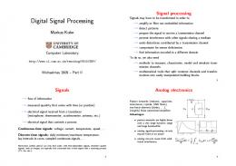
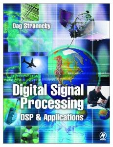
y[n] = yh[n] + yp[n] = A(2)n + Bn(2)n + C = (1/9)[7(2)n + 3n(2)n + 2(-1)n]u[n]. In the z-domain the solution is obtained by transforming the LCCDE and solving for the transfer function: H(z) = Y(z)/X(z) = z(z-1)/(z-2)2, Y(z) = X(z)H(z) = z2(z-1)/[(z+1)(z-2)2]. The inverse transform gives the same answer as y[n] above. Here we discuss the reason why it is important to understand signals/systems in both time and frequency domain. Later in designing IIR filters they can, for example, design different filters based on their pole/zero location an obvious characteristic evident in the frequency domain. At the same time students can use matlab solution to compare it to the analytical formulation presented above. >> n=0:1:10; >> B=[1 -1 0]; >> A=[1 -4 4]; >> x=(-1)^n; >> x=(-1).^n; >> y=filter(B,A,x) y= Columns 1 through 8 1
2
6
14
34
Columns 9 through 11 882
1934
4210
>> plot(n,y) >> xlabel ('n, Discrete-Time Index') >> ylabel('Total System Response, y[n]') >> title ('Example 1, IIR Complete Response') >> grid on >>
78
178
398
Example 1, IIR Complete Response 4500 4000
Total System Response, y[n]
3500 3000 2500 2000 1500 1000 500 0
0
1
2
3
4 5 6 n, Discrete-Time Index
7
8
9
10
Example 2. Here we ask students to design a lowpass digital filter based on a Butterworth approximation and given the following specifications: Passband cutoff frequency = 3 kHz, attenuation of at least 23 dB for F ≥ 6 kHz (note that capital letter is used for analog frequency.) We like to use a sampling frequency of 20 kHz. Although several methods are discussed in the class (in addition to CAD methods, we study backward/forward difference approximation, matched z-transform, impulse/step invariance), here we would like to use bilinear transformation method with pre-warping of frequencies. Using design formulas discussed in the lecture, it is found that the minimum filter order is N = 3, so that normalized analog filter is H(s) = 1/[(s + 1)(s2 + s +1)] Which can be transformed to obtain the digital design H(z) = (z + 1)3/[(3z – 1)(7z2 -6z + 3)].
Note that other analog approximation (e.g., Chebyshev I) can also be used. Here we present simulation results using MATHCAD.
H( ω) :=
z( ω) := exp( j⋅ ω)
j := −1
ω := 0 , 0.01.. π
( z( ω) + 1)3
(
)
⎡⎣( 3⋅ z( ω) − 1) ⋅ 7⋅ z( ω) 2 − 6⋅ z( ω) + 3 ⎤⎦ 1
H ( ω ) 0.5
0
0
0.5
1
1.5
2
2.5
3
3.5
ω
4 2 arg( H( ω ) ) 0 2 4
0
0.5
1
1.5
2
2.5
3
3.5
ω
Example 3. In designing FIR filter one approach is to use truncation (windowing) and finite delay of the ideal (desired) impulse response function. For the ideal digital lowpass filter given as Hd(ω) = 1 for – ωc≤ ω ≤ ωc, one gets the desired impulse response hd[n] = [ωc/π] Sa (ωcn), -∞ < n < ∞; where sampling function Sa(x)=(sin x)/x. Obviously this filter has ∞ duration (it is also non-causal.) The solution will be to use windowing and finite delay. We will illustrate this design method by designing a digital
FIR differentiator (not an easy analog design or IIR.) For ideal digital differentiator, the desired impulse response is given by hd[n] = cos(πn)/n, -∞ < n < ∞ with hd[0] = 0. We use MATHCAD simulation below to show a couple typical designs using Hanning and Kaiser windows. For Kaiser window with shape parameter β = 5 , we use the paper by Blachman and Mousavinezhad [5] to evaluate the zeroth-order modified Bessel function of the first kind: _ I0(x) ≈ 1/6 + (1/3) cosh(x/2) + (1/3) cosh(√3 x/2) + (1/6) cosh(x). ω := 0 , 0.01.. π
hd ( n ) :=
j := −1
n := 1 , 2 .. 100
cos ( π⋅ n ) n
w( n ) := 0.5 + 0.5⋅ cos ⎛⎜ π⋅
⎞ ⎟ ⎝ 100 ⎠ n
Hamming Window
∑ (hd (n)⋅ w(n)⋅sin (n⋅ω))⎥⎤
H( ω) := −2⋅ j⋅ ⎡
⎢ ⎣n
⎦
I0( x) :=
⎛
1 6
I0⎜ β ⋅ 1 − wk( n ) :=
⎝
+
1 3
⋅ cosh ⎛⎜
x⎞
1 1 ⎛ x⎞ ⎟ + ⋅ cosh ⎜ 3⋅ 2 ⎟ + ⎝ 2⎠ 3 ⎝ ⎠ 6⋅ cosh ( x)
β := 5
⎞ ⎟ 10000⎠ n
2
I0( β )
∑ (hd (n)⋅ wk(n)⋅sin (n⋅ω))⎤⎥
Hk( ω) := −2⋅ j⋅ ⎡
⎢ ⎣n
⎦
4 4 3 3 H( ω ) 2 Hk( ω ) 2 1 1 0
0
1
2
ω
3
4 0
0
1
2
ω
3
4
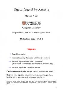
Real-Time Digital Signal Processing Implementation Considerations Computational Efficiency Fast algorithms of digital signal processing become imperative when students work on class projects of real-time applications. Projects are designed that allow students to implement DSP algorithms either on DSP development boards or on general-purpose PCs. When general-purpose PCs are used, high-level programming puts additional computational burden on the processor. It is critical to make the DSP algorithm efficient in order to meet real-time requirements. TRANSMITTER
RECEIVER
Receiving Thread Signal Reception
Processing Thread DSP Algorithms
Circular Buffer
Audio Cable
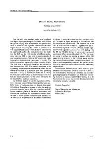
Figure 1. A platform that evaluates computational efficiency of DSP implementation.
For example, one class project is to simulate a signal generator and a frequency analyzer using two PCs (Figure 1). It is programmed in C++. The first PC generates a continuous signal that consists of N frequency components according to user input. The digital signal is fed to the computer audio card that functions as a D/A converter. The audio card has a predetermined sampling rate and outputs an analog waveform of the signal. The signal is transmitted through an audio cable, which is also plugged in the audio input of the other PC. The other PC receives the analog signal through the audio input port and uses the computer audio card as an A/D converter. The receiving PC can perform a series of DSP algorithms on the sampled signal. A simple manipulation of the received data is to perform discrete Fourier transform and detect the N frequency components in the original signal. There are a few practical issues in this programming task. First, because the sampling rate at the transmitting PC is determined by the selection of the audio card sampling rate, the signal generator has to reject input frequencies that do not satisfied the Nyquist requirement. Secondly, in order not to lose any data at reception, a multi-threaded program is necessary at the receiving PC. One thread, called receiving thread, takes the data in from the audio card, while the other thread, called processing thread, performs Fourier transform and detects the N largest peaks with their corresponding frequencies.
These two threads share a common circular buffer with its associated synchronization mechanism. When the DPS algorithms are computationally heavy in the processing thread, it may not be able to finish processing the data before new data flushes in from the audio input port. The students are made aware of this phenomenon of data loss due to inefficient DSP algorithms. And, they are encouraged to make modifications to the algorithms so that the data processing is completed before the circular buffer would overflow. A straightforward solution to this problem is to implement a fast Fourier transform algorithm. Students can try various FFT algorithms that include decimation-in-time and decimation-in-frequency FFT algorithm, and with various bit orders in the FFT butterfly graph1. Digitization Effects and System Stability The digitization effects come in the forms of sampling aliasing and quantization error. The sampling aliasing can be demonstrated in the above example of the class project. The quantization error can be classified as signal quantization errors and filter coefficient quantization errors. In DPS implementations, the arithmetic roundoff noise and the overflow effect should also be considered. After sampling, the discrete-time signal x(nT) is encoded using B-bit wordlength to obtain the digital signal x(n). We assume that −1 ≤ x(n) < 1, thus a dynamic range of 2. Since the quantizer employs B bits, the number of quantization levels is 2B. The quantization resolution, i.e. the spacing between two successive quantization levels, is Δ = 2/2B = 2-B+1 The sampled value x(nT) is rounded to the nearest level of a B-bit word. The quantization error e(n) cam be expressed as e(n) = x(n) − x(nT ) It is clear that |e(n)| ≤ Δ/2 The quantized signal can be expressed as x(n) = x(nT ) + e(n) For an arbitrary signal with fine quantization (B is large), the quantization error e(n) is assumed to be uncorrelated with x(n), and is a random noise that is uniformly distributed in the interval [−Δ/2, Δ/2]. Therefore, e(n) is zero mean with variance σe2 = 2-2B/3. Therefore, the signal-to-quantization-noise-ratio (SQNR) can be expressed in dB as
SQNR = 10 log10(σx2/σe2) = 4.77 + 6.02B + 10 log10σx2 Where, σx2 denotes the average signal power. This equation indicates that for each additional bit used, the quantizer provides about 6-dB gain.
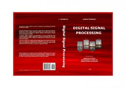
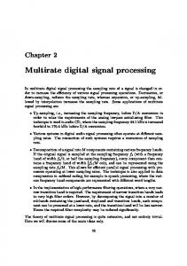
Figure 2. MATLAB example of quantization effect.
Figure 3. MATLAB example of overflow (saturation) effect.
Effects of signal quantization may be subjectively evaluated by observing and listening to the quantized audio signal. In a classroom demonstration of the quantization effects, we use MATLAB to read in a song wave and play it back on the speaker. The original audio signal, x(nT), is quantized with different resolutions. The quantized audio signal, x(n), is also played back on the speaker to compare with the original one. Fig. 2 shows portions of the signal waveforms of the original audio signal x(nT) and the quantized audio signal x(n). In this figure, the quantizer has B = 3 bits, and Δ = 2-B+1 = 0.25. With the same original audio signal, we can also demonstrate the overflow or saturation effect in DSP implementations. The saturated signal waveform is also played back using MATLAB on the speaker, and compared with the original audio signal. Fig. 3 shows the original audio waveform and the saturated waveform. The graphs and audio demonstrations provide students with a good understanding of the quantization and saturation effects. Another DSP implementation consideration is the filter coefficient quantization effect. The filter coefficients of the digital filter determined by a filter design package such as MATLAB are usually represented using the floating-point format. When implementing a digital filter, the filter coefficients have to be quantized for a given fixed-point processor. Therefore, the performance of the fixed-point digital filter will be different from its design specification. The coefficient quantization effects become more significant when tighter specifications are used, especially for IIR filters. Coefficient quantization can cause serious problems if the poles of designed IIR filters are too close to the unit circle. This is because those poles may move outside the unit circle due to coefficient quantization, resulting in an
unstable implementation. Such undesirable effects are far more pronounced in high-order systems. The coefficient quantization is also affected by the structures used for the implementation of digital filters. For example, the direct-form implementation of IIR filters is more sensitive to coefficient quantization than the cascade structure consisting of sections of first- or second-order IIR filters6. Real-time DSP application examples on an unstable system that results from coefficient quantization errors are provided in class. Conclusions Balancing theory and practice is important in many engineering subjects, especially those that have a lot of mathematical concepts and abstractions. The study of digital signal processing and its application is vital to the curriculum of electrical and computer engineering. Within the related courses, we have provided students with software packages for DSP demonstration and simulations, and with hardware/software platforms for DSP implementation on small projects. These tools have proved to be interesting and useful for the students to grasp fundamental knowledge in DSP. We have shown some actual classroom examples and homework assignments in both theory and practice. A laboratory component in digital signal processing is highly recommended for senior classes. Our university has a relatively long history of offering classes in DSP at both undergraduate and graduate level with emphasis on class projects and laboratory handson experience. We believe that it is important to introduce modern tools and software packages at the right time, right place. Bibliography 1. “Discrete-Time Signal Processing,” second edition, A. V. Oppenheim, R. W. Schafer, J. R. Buck, Prentice Hall, 1999. 2. “Digital Signal Processing, Principles, Algorithms, and Applications,” fourth edition, J. G. Proakis, D. G. Manolakis, Prentice-Hall, 2007. 3. “Signal Processing First,” J. H. McClellan, R. W. Schafer, M. A. Yoder, Prentice-Hall, 2003. 4. “The Scientist and Engineer’s Guide to Digital Signal Processing,” S. W. Smith, California Technical Publishing, www.dspguide.com, 1997. 5. “Trigonometric Approximations for Bessel Functions,” N. M. Blachman, S. H. Mousavinezhad, IEEE Transactions on Aerospace and Electronic Systems, 1986. 6. “Real-time digital signal processing: Implementations and applications,” S. M. Kuo, B. H. Lee, and W. Tian, second edition, John Wiley & Sons, 2006.