Digital Signal Processing with FPGAs

university of applied sciences hamburg

DEPARTMENT OF ELECTRICAL ENGINEERING AND COMPUTER SCIENCES

Prof. Dr. B. Schwarz

Handout

Digital Signal Processing with FPGAs

20 Bit Audio Codec

Field Programmable Gate Array (FPGA)

IE8 elective course 2. Edition SS 2004

Analog Stereo In/Out

XSTend Board + XC2S50 Spartan

Magnitude

Phase

1

180

0.8 90

|G(f)|

φ in degree

0.6

0.4

0

-90 0.2

0 0.4

0.8

1.2 f in Hz

1.6

2 x 10

-180 0.4

0.8

1.2 f in Hz

4

1.6

2 x 10

4

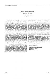
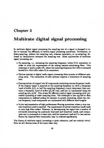
Group delay 900 Chebyshev I bandpass filter 4th order.

τ in µs

800 700

Nyquist frequency fN = 24kHz

600

Passband deviation Rp = 3dB

500 Passband frequencies: 400 fc /fN = [0.4 0.6]

300 200 100 0 0.4

0.8

1.2 f in Hz

1.6

2 x 10

4

DSP with FPGAs

1




Contents Introduction 1.1 Digital Filters 1.2 Fixed Point Hardware 1.3 Filter Example 1.4 Learning Outcome 1

2 2.1 2.2 2.3

FIR Filter: Design and Structures Linear Phase Response FIR Design with Window Method Direct and Transposed Forms 2.3.1 Direct Form I 2.3.2 Direct Form I with Reduced Number of Multipliers 2.3.3 Transposed Form 2.4 Fixed Point arithmetic implementation with VHDL and Filter Scaling 2.4.1 Fractional Binary Numbers; Q Format 2.4.2 Multiplication with Q Format Multiplier and Multiplicand 2.4.3 VHDL Model of a FIR Filter with Direct Form I Serial Structure with MAC Resource Sharing 2.4.4 2.5 Concepts of Multirate Signal Pocessing with Parallel Filter Structures

3 IIR Filter Design and Implementation 3.1 3.2 3.3 3.4 3.5 3.6 3.7

Coefficient Calculation with Bilinear z-Transformation (BZT) Filter Design with Classical Analog Filter References Realisation Structures: Parallel and Serial Solutions Cascade Structures for Higher Order Filters and Scaling Q-Format Vector Representation with VHDL Models for SOSs Finite Coefficient Word Length Effects Sine Wave Generator

4 Goertzel Algorithm for Frequency Detection 4.1 4.2

Basic DFT Equations and DFT Coefficients Second Order Decimation IIR Bandpass with Power Estimation

5 FPGA Platform with Audio Signal Interface 5.1 XST-1 XSTend Board 5.2 AK4520A 20 Bit Codec 5.3 XSA-50 Board with Spartan-II FPGA

Laboratory Exercises 6.1 FIR Serial Structure with one MAC Unit, Samples and Coefficient FPGA-RAM 6.2 IIR ChebyshevI 6th Order Bandpass with Cascaded SOS 6.3 FIR Filter Types with Parallel Structure; Transposed Form; Reduced Multipliers

6

DSP with FPGAs

2

university of applied sciences hamburg Prof. Dr. B. Schwarz


Literature [1]

E. C: Ifeachor; B. W. Jervis: Digital Signal Processing. A Practical Approach. Prentice Hall 2nd edition 2002.

[2]

St. W. Smith: The Scientist and Engineer’s Guide to Digital Signal Processing. California Technical Publishing. San Diego Ca. 2nd edition 1999. pdf-files available from www.dspguide.com. Copyright ©1997-1998 by Steven W. Smith.

[3]

R. G. Lyons: Understanding Digital signal Processing. Prentice Hall 2001.

[4]

A. Bateman; I. Paterson-Stephens: The DSP Handbook. Algorithms, Applications and Design Techniques. Prentice Hall 2002.

[5]

U. Meyer-Baese: Digital Signal Processing with Field Programmable Gate Arrays. Springer Verlag 2001.

[6]

D. Ch. v. Grünigen: Digitale Signalverarbeitung. Fachbuchverlag Leipzig/Hanser Verlag, 2. Auflage 2002.

[7]

K. D: Kammeyer; K. Kroschel: Digitale Signalverarbeitung. Filterung und Spektralanalyse mit MATLAB-Übungen. Teubner Studienbücher Stuttgart, 4. Auflage 1998.

[8]

U. Zölzer: Digitale Audiosignalverarbeitung. Teubner Stuttgart 2. Auflage 1997.

[9]

M. Werner: Digitale Signalverarbeitung mit Matlab. Vieweg Verlag 2001.

[10]

R. Gazit: Create Efficient FIR Filters using Virtex and Spartan FPGAs. Xilinx Xcell Journal Issue 38, 4th Quarter 2000. www.xilinx.com → Literature, Xcell Journal Archives or Application Notes (XAPPijk)

[11]

J. Villasenor; B. Hutchings: The flexibility of configurable computing. IEEE Signal Processing Magazine, page 67-84 1998.

[12]

XST-1 Xstend Board V1.3.2 Manual. XESS Corporation 17.05. 2001. www.xess.com → products , manuals

[13]

AKM Codec AK4520A data sheet. ASAHI KASEI 1997/3.

[14]

A. Burr: Modulation and Coding for Wireless Communication. Prentice Hall, Pearson Education 2001.

[15]

Matlab: Signal Processing Toolbox: The Mathworks User’s Guide documentation, pdf-file available with the Help function.

[16]

D. G. Manolakis; V. K. Ingle; St. M. Kogon: Statistical and Adaptive Signal Processing. McGraw Hill International Editions 2000.

[17]

S. K. Mitra: Digital Signal Processing. McGraw Hill 2001.

DSP with FPGAs

3



1 Introduction Digital signal processing has a major and increasing impact in key areas of technology, i.e. telecommunication, digital television, media and digital audio. The need and expectations for electronic, computer and communication engineers to be competent in DSP have grown. Many frontend DSP algorithms such as FFTs, FIR and IIR filters previously build with programmable signal processors are now replaced by FPGAs [11]. Modern FPGA devices provide DSP arithmetic support with fast-carry chains which are used to implement multiply-accumulate (MACs) with high speed and small hardware amount. Additional 18x18 bit multipliers in direct neighbourhood to internal block RAM support highly parallel operation of typical coefficient-sample products. This course provides an enhancement of digital system development knowledge about transformations of mathematical based topics to fixed point applications with FPGA hardware. The main targets which are covered by this course for students with advanced skills in VHDL synthesis aim on preparation for master thesis projects which are related to following topics: • Implementation of signal processing algorithms in mobile communication components: Speech coding, source coding, channel coding with error correction abilities, modulation technology. • Image processing for object identification: contrast enhancement, edge detection and linear/non linear filtering, segmentation for object-background separation. With advanced knowledge about digital system design based on reconfigurable hardware master thesis cooperation with many involved professors will be supported.

1.1 Digital Filters Digital filters are among the most significant components in digital signal processing applications. The function of a filter is to eliminate undesirable parts of the signal (random noise), or to extract signals in a particular frequency range. In other words, a filter selects, suppresses, or modifies certain frequency components of the signal, either to reduce noise or to shape the spectrum. This course focuses on digital filters that are used widely in digital video broadcast, digital video effects, digital wireless communication and audio signal processing. An application example of Finite Impulse Response (FIR) filters in a wireless communication receiver is depicted in Fig. 1-1. In digital audio broadcasting (DAB) and DVB system the quadrature amplitude modulation (QAM) is implemented because of its bandwidth efficiency [14]. The QAM demodulator regenerates the baseband signal from the modulated signal at the 2. intermediate frequency (IF) stage. The demodulator contains two arms, one uses a cosine wave (in phase with the carrier) and the other a sine wave (in quadrature with it). These arms reconstruct the inphase I and quadrature Q components of the modulated signal by suppressing the carrier with high order FIR low pass filters. The non recursive FIR type is required for this attenuation because the recovered baseband pulses may be delayed but no phase distortion is allowed which would disturb the process of symbol detection. A broad survey to digital signal processing applications is provided by chapters in [1, 2, 3, 4, 5, 15]. Most of the traditional filters in DSP applications are implemented using highly specialized DSP processors. These DSP processors are capable of carrying out high-speed Multiply Accumulate

DSP with FPGAs

4



Fig. 1-1: Radio receiver with FPGA based DSP for QAM coherent demodulation[10; XAPP 219 01.10.2001].

(MAC) operations, but have bandwidth limitations. Only a fixed number of operations can be performed by these processors before the next sample arrives, thereby limiting the bandwidth. DSP processors are sequential in nature, and thus DSPs using a single processor can only perform one operation on a single set of data at a time. For example, in a 16-tap (register stage) filter, they can only calculate the value of a single tap at a time, while the other 15 taps wait for their turn. This also limits the overall frequency of the application. Due to resource limitations, operations cannot be performed in parallel. FPGA based filters are implemented with parallel-pipelined architecture, enhancing the overall performance [5, 10]. Hence it is an important step during digital signal processing system design to decide which implementation structure should be chosen in order full fill requirements according allowed use of FPGAs or ASICs HW resources and meet the needed clock frequency. Besides the knowledge about mathematical background of filter design methods it is crucial to be experienced in HDL modelling of reliable filter arithmetic.

1.2 Fixed Point Hardware Within digital hardware, numbers are represented as either fixed-point or floating-point data types. For both these data types, word sizes are fixed at a set number of bits. However, the dynamic range of fixed-point values is much less than floating-point values with equivalent word sizes. For example with 32-bit fixed point representation the 232 quantisation levels spaced uniformly over a relatively small range, say for Q31 format, between -1 and 1 with gaps of 1 LSB = 2-31. In comparison, floating point notation places the 232 quantisation levels logarithmically over a huge range, typically ±3.4×1038.

DSP with FPGAs

5



This gives 32-bit fixed point better precision, that is, the quantisation error on any one sample will be lower. However, 32-bit floating point has a higher dynamic range, meaning there is a greater difference between the largest number and the smallest number that can be represented. In fixed point the possibility of an overflow needs to be considered after each operation. The designer needs to continually understand the amplitude of the numbers, how the quantisation errors are accumulating and what scaling of outputs have to be applied. Since floating-point HW can greatly simplify the real-time implementation of a digital filter, and floating-point numbers can effectively approximate real-world numbers, then why use a DSP or FPGA with fixed-point hardware support? For FPGAs and ASICs there is no other choice than to start with implementations of arithmetic and algorithms based on integer and fractional number representation. The reason is that the HDL modelling libraries only offer unsigned and two’s complement signal types which are supported for HW synthesis. On the other hand fixed point gives the flexibility to decide which vector width for number representation is necessary in order balance precision (size of gaps between numbers) and amount of implemented HW resources (adder, multiplier and register width). For DSPs the answer to this question in many cases is cost and size Fig. 1-2: •Cost Fixed-point hardware is more cost effective where price/cost is an important consideration. When using digital hardware in a product, especially mass-produced products, fixed-point hardware, costing much less than floating-point hardware, can result in significant savings. •Size The logic circuits of fixed-point hardware are much less complicated than those of floating-point hardware. This means the fixed-point chip size is smaller with less power consumption when compared with floating-point hardware. For example, consider a portable telephone where one of the product design goals is to make it as portable (small and light) as possible. If one of today’s highend floating-point, general purpose processors is used, a large heat sink and battery would also be needed resulting in a costly, large, and heavy portable phone. After making the decision to use fixed-point hardware, the next step is to choose a method for implementing the dynamic system. Floating-point emulation libraries are generally ruled out because of timing or HW resource consumption constraints. Therefore, you are left with fixed-point math where binary integer values are scaled. Fig. 1-2: Fixed versus floating point. Fixed point DSPs are generally cheaper, while floating point devices have higher dynamic range, and a shorter development cycle [2, chapter 28 and 4].

DSP with FPGAs

6




1.3

Filter Example

Linear digital filters typically come in two flavours: finite impulse response (FIR) filters and infinite impulse response (IIR) filters. Two examples are presented in the following in order to give a taste of typical terms like averaging, convolution and linear phase response. FIR filters use only current and past input samples and none of the filter’s previous output samples, to obtain a current output sample value. Therefore FIR filters are also called nonrecursive filters. FIR filters use addition to calculate their outputs in a kind as the process of averaging uses addition. With the example in Fig. 1-3 the counted number of cars that pass over a bridge every minutes is depicted. The average number of cars per minute over five minute intervals is calculated by Eq. 1-1 with the number of used measurements N+1 = 5. Four stored old values and the latest update x[n] are averaged, and yield the newest result y[n]. N

y ( n ) = 0 .2 ∑ x ( n − k )

1-1

k =0

Until the fifth measurement has been sampled at time t = 4 minutes the average process was filled with five incoming samples so that the first average value y[4] = 47 becomes valid. From that time on a new sample is include and the oldest namely former x[n-4] is deleted. One important effect of average process is that sudden changes of the input sequence x are flattened out. The calculated output sequence y is much smoother because high frequencies of the input x are suppressed.

Fig. 1-3: Averaging the measured cars/minute number. The blue curve with squares gives the average over the last five minutes. Random input signal x with mean value 50 and variance 100.

This low-pass filter behaviour is provided by a FIR filter characteristic because only input values have been evaluated, previous ones and the newest sample update. No previous averager output is used for calculations of the current output. The low-pass behaviour becomes apparent again when the bridge is closed immediately at time t = 24 minutes. The next sample x[25] is zero and the FIR

DSP with FPGAs

7




output is degrading with delay for another 4 minutes until t = 29. The averager can be described with a filter structure like Fig. 1-4 which calculates a new output from left to right along the single

49

45

48

60 47.8

37

Fig. 1-4: Averager block diagram of 4th order with h(k) = 0.2. The first five samples x are applied at time t = 4 minutes.

delay stages 1 to 4. The delay elements represent unit delays which are marked with z-1 the ztransform variable one sample interval delay. These delay blocks indicate shift registers where input samples are stored with every rising edge of a sample clock signal. With each new input to the first delay block the output sum of all taped delay blocks is updated and weighted with the gain 0.2 . One of the most important aspect of understanding filters is how to predict their behaviour when sinusoidal input samples of different frequencies are applied to the input: frequency domain response. In order to recognise the influence of parameters like the number of delay elements and the chosen weighting gains the evaluation of the z-transform transfer function will be analysed which gives a description of the discrete time domain behaviour. With the knowledge of the discrete fourier transform (DFT) at a later stage the mathematical handling of filters will be completed. The general description of FIR filters with separate weighting gains h[k] for each delay stage is given with the difference Eq. 1-2 where N is the number of stages and L = N +1 the length of the filter and the number of coefficients h[k].

y (n) =

N

∑ h(k ) x(n − k ) k =0

1-2

By applying a single pulse x(n) to the FIR filter the output becomes the impulse response which is made up by a sequence of y(n) samples which are equal to the coefficients h(k). The corresponding z-transform transfer function H(z) is as follows whereby the time shift property is applied which is widely used in converting the z transfer function into difference equations and vice versa: N

Y ( z ) = ∑ h( k ) z − k X ( z ) = H ( z ) X ( z ) k =0

1-3

This Eq. 1-3 can be applied to the 4th order averager according to Fig. 1-4 with general coefficients h(k):

DSP with FPGAs

8




H(z) = h(0) + h(1)z-1 + h(2)z-2 + h(3)z-3 + h(4)z-4

1-4

In order to introduce an important class of FIR filters symmetrical coefficients are chosen which will provide a linear phase response:

h(k)= h(N – k) positve symmetry h(k)= -h(N – k) negative symmetry

1-5

By grouping the delay terms in transfer function Eq. 1-4 with positive symmetry coefficients it results:

H(z) =z-2{ h(0)(z2 + z-2) + h(1)(z-1 +z-1) + h(2)}

1-6

The frequency response H(ω) describes the filter properties as a response to single input sinewave signal with frequency f which are used to excite the input and observe the output signal by comparing amplitudes and phase shift: continuous excitation. No transitions of input signals from one stationary state to another are regarded. Therefore the substitution z = ejωT can be applied and reductions with Euler’s relationships are possible. The rotational frequency ω = 2πf is measured in radiants/second and the delay time T = 1/fS represents the sampling period:

H(ω) = e -j2ωT{2h(0)cos2ωT + 2h(1)cosωT + h(2)}

1-7

This closed expression Eq. 1-7 describes both magnitude and phase as a function of ω for the FIR filter with order N = 4: Phase: Magnitude:

∠ H(ω) = -2 ωT |H(ω)| = |2h(0)cos2ωT + 2h(1)cosωT + h(2)}|

1-8

With Fig. 1-5 a) the low-pass behaviour of the averager filter becomes evident but it is far away from an ideal low-pass which should have a steep transition of |H(ω)| from pass band to stop band. Especially the poor attenuation right from the first zero which is characterised by sidelobes is not satisfying. In order to develop a better view to parameters influence on the frequency behaviour the zeros of |H(ω)| can be calculated in which some trigonometric identities have to be used:

|H(ω)| = 4h(0)cos2ωT + 2h(1)cosωT + h(2) - 2h(0)}= 0

1-9

This quadratic equation for cosωT can be solved to evaluate the ω position of the |H(ω)| sidelobes:

cos ω T 1 / 2

1 h (1 ) = − ± 4 h (0 )

1 16

(

h (1 )

⎛ h (2 ) − 2 h (0 ) ⎞ ⎟⎟ − ⎜⎜ ) h (0 ) 4 h (0 ) ⎠ ⎝ 2

1-10

D DSP with FPGAs

9



a)

ω2 b)

Fig. 1-5: Averaging filter frequency response with h(k) = 0.2, T = 60 sec ( fS/2 = 0.05236 rad/sec) and N = 4 . |H(ω)| frequency magnitude response a), ∠H(ω) phase angle response of H(ω) b).

With the condition D ≥ 0 the square root assures that real root values of cosωT exist to which zeros of the magnitude response with total attenuation belong. With equal h(k) values the zeros of |H(ω)| are fixed at ω locations which depend on the order N of the Filter. With a 4th order averager we receive:

cosωT1/2 = -0.25(1 ± 51/2): f1 = 0.2fS , ω1 = 0.0209rad/s; f2 = 0.4fS , ω2 = 0.0419rad/s; 1-11 The maximum values of the sidelobes are derived by the first derivative dH(ω)/dω set to zero. Applied to Eq. 1-9 we receive three ωm values:

ωm1 = 0 : |H(0)| = ∑ h(k) = 1; DC gain 1-12 ωm2 = π fS: |H(fS/2)| = |2h(0) –2h(1) +h(2)| = |1 – 4h(1)| = 0.2 ωm3 = fS arcos(-0.25h(1)/h(0)) = 0.03039 rad/s: |H(ωm3)| = |-0.25h(1)2/h(0) + h(2) –2h(0)| = |-0.25| Besides these discussion of the magnitude frequency response the phase frequency response in b) has to be recognised as a linear phase response. In the pass band interval 0 ≤ ω ≤ ω1 the phase of the 4th order averager follows according to Eq. 1-8 ∠ H(ω) = -2 ωT.

DSP with FPGAs

10




Therefore all input signal frequency components will be delayed with the same amount of delay time which is called group delay τgr and represents the negative slope of the phase response:

τgr = - d∠ H(ω)/dω = 2T

1-13

In general it will be developed in chapter 2 that FIR filters with order N and symmetrical coefficients will provide a constant group delay of certain number of sample periods τgr = TN/2. The phase discontinuities at ω1/2 arise from the fact that the expression of Eq. 1-6 in {~} brackets changes its sign and therefore introduces another phase shift of ± 1800 . So far it has been recognised with this first simple FIR filter example which is made of equal coefficients h(k) = = 0.2 and order N = 4 that: • The pass band is fixed to ω1 and the sidelobes as well to ω1 and ω2 . • The unattractive sidelobe magnitudes are related to the DC gain of ∑ h(k) = 1. A small step in a direction to change the filter’s frequency response will be done by changing the coefficients in a way that there is a maximum value with h(2) and lower values for the other h(k). As an effect the impulse response of this filter will have less abrupt transitions and the sidelobe ripples in the frequency response are reduced (comp. Eq. 1-8). In order preserve the zeros of |H(ω)| which support the characteristic of a pass band the condition D ≥ 0 in Eq. 1-10 has to be obeyed and additionally ∑ h(k) = 1 should be fulfilled. With a given value for h(2) = 0.4 the evaluation of D ≥ 0 will provide a suggestion for h(1): 2h(0) + 2h(1) = 1 – h(2) = 0.6 yields h(0) = 0.3 – h(1) D ≥ 0: h(1)2 + 8h(1)h(0) –4h(0) +8h(0)2 ≥ 0 h(1) ≥ 0.2583 ; h(0) = 0.3 – h(1) ≤ 0.0417

1-14

With this coefficient estimation the FIR block diagram Fig. 1-6 depicts weighted delay element outputs which contribute to the filter’s sum.

Fig. 1-6: FIR filter structure 4th order with symmetrical coefficients.

DSP with FPGAs

11



Fig. 1-7: FIR filter frequency response with h(0) = 0.04, h(1)=0.26, h(2)=0.4, T = 60 sec ( fS/2 = 0.05236 rad/sec) and N = 4 . |H(ω)| frequency magnitude response a), ∠H(ω) phase angle response of H(ω) b).

By evaluating Eq. 1-10 and Eq.1-12 the results in Eq. 1-15 confirm the magnitude and phase response in Fig. 1-7. With reduced h(0) coefficient the sidelobe is flattened but the pass band frequency range has a very flat magnitude transition. cosωT1 = -0.825: f1 = 0.404fS , ω1 = 0.0423rad/s; only one zero ωm1 = 0 : |H(0)| = ∑ h(k) = 1; DC gain ωm2 = π fS : |H(fS/2)| = |2h(0) –2h(1) +h(2)| = |1 – 4h(1)| = 0.04

1-15

From these examples it can be seen that design rules are necessary which provide an access to filter coefficients by given pass band corner frequencies and filter order in order to receive a steep transition from pass band to stop band and increase the attenuation of the sidelobes.

DSP with FPGAs

12




Now a review of time domain behaviour should follow because the infamous term convolution can be made clearer with some pencil and paper activities. Again Eq. 1-1 and 1-2 are regarded and for each single time step (sample period) of an example FIR filter output with four coefficients and order N = 3 can be written:

y(n) = h(3)x(n-3) + h(2)x(n-2) + h(1)x(n-1) + h(0)x(n)

1-16

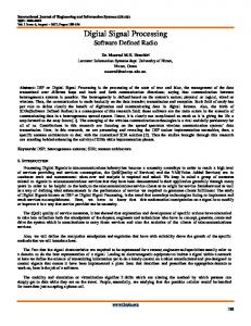
From this equation it can be seen that there is an immediate reach through of the current input x(n) to the output y(n) even if a pure low pass filter is implemented. That is totally different from continuous time domain filter descriptions with laplacian transfer functions for low pass filters. With Eq. 1-16 each output signal sample y(n) will be calculated beginning with the first input x(0) until the last input sample x(M-1) of an input sequence with M samples has been combined with h(3). A scheme for a convolution machine will support the understanding of the summation of a series of products [2, chapt. 6]. It has to be noticed with Eq. 1-2 that for a given y(n) the h(k)’s index is increasing as the x(k)’s index is decreasing which means that previous inputs before x(k) have to be used. Therefore the scheme introduced in [2] (comp. Fig. 1-8 - Fig. 1-12) uses an impulse response which is flipped left-for-right so that h(0) is on the right hand side of the k axis. According to example Eq. 1-16 x(n) samples are aligned with the coefficients h(k) for a given n index to calculate y(n). In Fig. 1-9 the Eq. 1-16 is represented on the right half for y(n = 3). This scheme for an convolution machine represents the view to individual output samples and finding the contributing points from the input through the h(k) pattern. The convolution process is continued by shifting the h(k) pattern to the right and including a newer x(k) into the sum of products. There is a problem given with the start of the process Fig. 1-8 and the final operation in Fig. 1-12. In Fig. 1-8 the convolution machine is located on the left with its output aim to y(0) but three older inputs x(-1), x(-2) and x(-3) don’t exist. A similar condition is apparent in Fig. 1-12 where future values x(8), x(9) and x(10) are not available because the input sequence has finished. This problem is solved by adding samples to the ends of the sequence with a value of zero. As a consequence beginning and ending output samples have to be regarded disregarded. In the general case if h(k) is a N+1 (length) point pattern running from 0 to N and x(k) is a M+1 (length) point signal running from 0 to M-1 then the convolution of the two is a N+M+1 point signal y(n) running from 0 to N+M. This set of equations for y(n) is described with the convolution star *, which is a mixture composed of the adder plus + and the multiplication cross x operators:

y(n) = h(k) * x(k)

1-17

The result from the convolution example depicted in Fig. 1-8 up to Fig. 1-12 shows that the implemented low pass FIR filter attenuates the amplitude so that the mean value of the input sequence x(k) is extracted.

DSP with FPGAs

13




x(k)

3 2 1 0 -1 -2 -3

3 2 1 x(k) 0 -1 -2 -3

0 1 2 3 4 5 6 7

X X X X

h(k) flipped

3 2 1 0

X X X X

0.4 0.3 0.2 0.1 0

h(k) flipped

3 2 1 0

+

3 2 1 y(n) 0 -1 -2 -3

0 1 2 3 4 5 6 7

0.4 0.3 0.2 0.1 0

+

0 1 2 3 4 5 6 7 8 9 10

3 2 1 y(n) 0 -1 -2 -3

0 1 2 3 4 5 6 7 8 9 10

Fig. 1-8: FIR low pass filter convolution: results y(0), y(1). Order N = 3, h(0) = 0.1 = h(3), h(2) = 0.4 = h(3).

DSP with FPGAs

14




x(k)

3 2 1 0 -1 -2 -3

3 2 1 x(k) 0 -1 -2 -3

0 1 2 3 4 5 6 7

X X X X

h(k) flipped

3 2 1 0

0 1 2 3 4 5 6 7 X X X X

0.4 0.3 0.2 0.1 0

h(k) flipped

3 2 1 0

+ 3 2 1 y(n) 0 -1 -2 -3

0.4 0.3 0.2 0.1 0

+

0 1 2 3 4 5 6 7 8 9 10

3 2 1 y(n) 0 -1 -2 -3

0 1 2 3 4 5 6 7 8 9 10


DSP with FPGAs

15




x(k)

3 2 1 0 -1 -2 -3

0 1 2

3 4 5 6 7

3 2 1 x(k) 0 -1 -2 -3

0 1 2 3 4 5 6 7

X X X X

h(k) flipped 3 2 1 0

X X X X

0.4 0.3 0.2 0.1 0


+ 3 2 1 y(n) 0 -1 -2 -3

0.4 0.3 0.2 0.1 0

+

0 1 2 3 4 5 6 7 8 9 10

3 2 1 y(n) 0 -1 -2 -3

0 1 2 3 4 5 6 7

8 9 10


DSP with FPGAs

16




x(k)

3 2 1 0 -1 -2 -3

3 2 1 x(k) 0 -1 -2 -3

0 1 2 3 4 5 6 7

0 1 2 3 4 5 6 7

X X X X


X X X X

0.4 0.3 0.2 0.1 0


+ 3 2 1 y(n) 0 -1 -2 -3

0.4 0.3 0.2 0.1 0

+

0 1 2 3 4 5 6 7 8 9 10

3 2 1 y(n) 0 -1 -2 -3

0 1 2 3 4 5 6 7 8 9 10


DSP with FPGAs

17




x(k)

3 2 1 0 -1 -2 -3

3 2 1 x(k) 0 -1 -2 -3

0 1 2 3 4 5 6 7

0 1 2 3 4 5 6 7

X X X X


X X X X

0.4 0.3 0.2 0.1 0


+ 3 2 1 y(n) 0 -1 -2 -3

0.4 0.3 0.2 0.1 0

+

0 1 2 3 4 5 6 7 8 9 10

3 2 1 y(n) 0 -1 -2 -3

0 1 2 3 4 5 6 7 8 9 10

Fig. 1-12: FIR low pass filter convolution: results y(8), y(9), y(10). Order N = 3, h(0) = 0.1 = h(3), h(2) = 0.4 = h(3).

DSP with FPGAs

18


3.1


Learning Outcome

The aim of this course covers the understanding and the ability to apply a complete design flow for FPGA implementation of digital filters with fixed point arithmetic. The knowledge of FIR and IIR filter design steps for selected filter types will be provided with Matlab functions and the fundamental mathematical background. Especially the finite word length effects which are introduced by fixed point hardware should be understood and further be regarded as conditions with each step of design flow and final hardware implementation. An important target of this lesson and laboratory based course is to support students with criterions for an appropriate choice of filter structures for parallel hardware implementations and sequential realisations with resource sharing of MAC units. Typical conditions which have to be understood and regarded during filter implementation with two’s complement arithmetic are as follows: • Minimisation of hardware resources by utilisation of symmetrical coefficient FIR filter properties. • Reduce long combinational logic signal path with balanced adder trees and pipelining. • Delay balancing needed with pipelining in high data rate applications. • Reuse of multiplication results in IIR filter transposed canonical form based on bilinear transform design. • Scaling of IIR filters implemented in cascade form with second order subblocks. • Application of guard bits in fixed point arithmetic in order to prevent overflow effects in scaled systems and to avoid harmonic distortion. • Realisation of MAC based resource sharing in systems with low sample frequencies. • Circular buffer implementation with FIR filters. • Mixed input signal and intermediate result storage in cascaded IIR SOS blocks with FPGA internal RAM. • Analysis of finite word length effects on quantisation noise in filter outputs. Finally filter implementations with a FPGA-Codec platform should be supported with a reasoning based on explanations of time domain and frequency response measurements.

DSP with FPGAs

19

Digital Signal Processing with FPGAs

Digital Signal Processing with FPGAs

Suggest Documents

Real-Time Digital Signal Processing Based on FPGAs for ... - MDPI

Applied Digital Signal Processing

Digital Signal Processing

digital signal processing - fmcet

Advanced Digital Signal Processing

Digital Signal Processing

BIOMEDICAL DIGITAL SIGNAL PROCESSING

Digital Signal Processing

Digital Signal Processing

digital signal processing

for Digital Signal Processing

Digital Signal Processing

Digital Signal Processing

ELEC3104: Digital Signal Processing

Digital Signal Processing

Digital Signal Processing

Multirate digital signal processing

Digital Signal Processing

Digital Communications and Signal Processing – with Matlab ...

Digital Signal Processing with General Purpose ... - AOE

EE 438 DIGITAL SIGNAL PROCESSING WITH APPLICATIONS

Biometric speech signal processing in a system with digital signal

Digital Signal Processing Pre-processing ... - Semantic Scholar

Understanding Digital Signal Processing - Pearsoncmg.com