JOURNAL OF PARALLEL AND DISTRIBUTED COMPUTING ARTICLE NO.
33, 98–106 (1996)
0029
Dilation-5 Embedding of 3-Dimensional Grids into Hypercubes M. Y. CHAN, F. CHIN,1 C. N. CHU, AND W. K. MAK Department of Computer Science, The University of Hong Kong, Pokfulam Road, Hong Kong
binary number, which effectively names the node in the optimal log2 abc-cube to which it is mapped. G can be seen as comprising of c layers of 2D grids each of size a 3 b. For the convenience of doing modulo arithmetics, we will adopt the convention of calling the first layer layer 0, the second layer layer 1, etc. This convention also applies to other terms such as ‘‘link’’ and ‘‘cell’’ to be defined later. Let l 5 2log2ab. To aid the assignment of binary labels to every node, we will partition G’s nodes into l groups, called links, evenly in the sense that when counting from layer 0 to layer k (0 # k # c 2 1), the number of nodes belonging to any particular link is either (k 1 1)ab/l or (k 1 1)ab/l. Partitioning G’s nodes into l links is equivalent to determining a unique pair of numbers for each node of G, namely, a link-number and a bead-number. A node’s linknumber indicates the link to which a node belongs, while its bead-number tells its position in that link. After the partitioning, we will use a node’s link-number to determine the first log2 l bits of its binary label, which we will call the link-label. And we will use a node’s bead-number to determine the remaining bits of its binary label, which we will call the bead-label.
We present an algorithm to map the nodes of a 3-dimensional grid to the nodes of its optimal hypercube on a one-to-one basis with dilation at most 5. 1996 Academic Press, Inc.
1. INTRODUCTION
A binary hypercube of dimension n is an undirected graph of 2 n nodes labeled 0 to 2 n 2 1 in binary where two nodes are connected if and only if their labels differ in exactly one bit position. Since a hypercube has a regular structure with a rich interconnection, it is a popular multiprocessor computer architecture. An embedding for a 3D grid into a hypercube can be viewed as a high-level description of an efficient method to simulate an algorithm designed for a parallel computer with a 3D grid structure on a parallel computer with a hypercube structure. Here we are interested in the problem of mapping the nodes of any 3D grid into nodes of its optimal hypercube (the smallest hypercube with at least as many nodes as the grid) on a one-to-one basis, so that dilation (the worst case distance between grid-neighbors in the hypercube) is bounded by a small constant. A related problem, namely, the problem of embedding 2D grids into hypercubes has been well studied by a number of researchers [BMS, BS, C1, C2, CC1, CC2, G, HJ, HLV, LS, SS]. It is known that every 2D grid can be embedded into its optimal hypercube with at most dilation 2 [C1, C2, HLV]. Since it has been proven that over 38% of all 2D grids need at least dilation 2 [BS], the methods proposed in [C1, C2, HLV] are optimal. However, not much is known about the optimal dilation for embedding 3D grids into optimal hypercubes. A nontrivial extension of the technique in [C1, C2] for embedding 3D grids into optimal hypercubes with at most dilation 7 was given by Chan in [C3]. A dilation-6 embedding scheme was derived later in [LH]. In this paper, we introduce a simple dilation5 embedding strategy for embedding 3D grids into optimal hypercubes.
3. PRELIMINARIES
In this section, we describe some basic results which we will make use of in our embedding strategy. In [HLV], a general embedding strategy for embedding 2D grids into 2D grids (of different sizes) was introduced. In particular, it can be used to embed an a 3 b guest grid into an a9 3 b9 host grid where a9 5 2log2a and b9 5 ab/a9. (Note that in [HLV], the embedding strategy was described for embedding an h 3 w guest grid into an h9 3 w9 host grid where w9 # w and h9 5 hw/w9; here we swapped the roles of row and column for later convenience.) As the embedding is one-one, a9b9 has to be greater than ab, and some nodes in the a9 3 b9 host grid do not correspond to any node in the a 3 b guest grid. A nice property of this embedding is that any unmapped node is only found in the last column of the a9 3 b9 host grid. So we can view the above embedding as one that embeds an a 3 b grid into a jagged grid of a9 rows where each row consists of either b9 or b9 2 1 nodes, and the total number of nodes of the jagged grid is exactly ab. Figure 1 shows an example of such an embedding. It is proven in [HLV]
2. GENERAL OUTLINE
Consider a 3D grid G of size a 3 b 3 c. Our objective is to label each node of G with a unique log2abc-bit 1
E-mail:
[email protected]. 98
0743-7315/96 $18.00 Copyright 1996 by Academic Press, Inc. All rights of reproduction in any form reserved.
DILATION-5 EMBEDDING OF 3D GRIDS INTO HYPERCUBES
99
FIG. 1. Transform a layer (rectangular grid) into a jagged grid by the trio method.
that this method yields a dilation-2 embedding for any a 3 b guest grid. A careful study of the proof will reveal that the method actually ensures that any two neighboring nodes in the a 3 b grid can only be mapped to one the following five sets of relative positions in the a9-row jagged grid: h[x, y], [x, y 1 1]j,
h[x, y], [x 1 1, y 2 1]j, h[x, y], [x 1 1, y]j,
GRAY(t, p) 5 ( p 1 1)th element of the t-bit binary reflected Gray code sequence.
h[x, y], [x 1 1, y 1 1]j. Here [x, y] denotes the position in row x, column y of the jagged grid. We will utilize this 2D grid embedding method as the first step of our embedding strategy for embedding 3D grids into optimal hypercubes, and we will refer to it as the trio method from now on. The process of partitioning G into l links depends on a length-l vector of 1’s and 2’s, v(a, b), or simply v. v is defined as follows [C2]. DEFINITION 1. Define
5
3
ab/l ab/l 2ab/l 2 ab/l 3ab/l 2 2ab/l ??? (l 2 1)ab/l 2 (l 2 2)ab/l
4
,
Basically, v is defined so that the 2’s are evenly distributed among the 1’s when there are more 1’s than 2’s and vice versa when there are more 2’s than 1’s. The vector v has a ‘‘cyclic sum’’ property which is stated below. DEFINITION 2. For 0 # s # l 2 1 and k $ 0, define [C2]
Ov
s1k21
i mod l
i 5s
For example, GRAY(3, 5) ; 111 since 111 is the sixth element of (000, 001, 011, 010, 110, 111, 101, 100). Fact 2 (Gray Code Property). In the t-bit binary reflected Gray code sequence, for any p such that 0 # p # 2 t 2 1 and for any i $ 0, the number of differing bits of GRAY(t, p) and GRAY(t, ( p 6 i) mod 2 t ) is at most i. The Gray Code Property above can be deduced from the fact that GRAY(t, p) and GRAY(t, ( p 6 1) mod 2 t ) differ in exactly one bit position for 0 # p # 2 t 2 1. 4. EMBEDDING STRATEGY
where l 5 2log2ab.
CYCLIC-SUM(s, k) 5
In determining the final binary label given to each node we will make use of the binary reflected Gray code sequence, a property of which is stated below. DEFINITION 3. For t $ 0 and 0 # p # 2 t 2 1, define
h[x, y], [x, y 1 2]j,
v(a, b) 5 [v0 , v1 , v2, ..., vl21]
Fact 1 (Cyclic Sum Property). kab/l # CYCLICSUM(s, k) # kab/l for 0 # s # l 2 1, k $ 0.
Let us first define the constants that will appear throughout the paper. They are l 5 2log2ab, a˜ 5 2log2a, and b˜ 5 l/a˜ . Throughout this section, we will use a 5 3 5 3 5 grid as a running example. To partition the nodes of an a 3 b 3 c grid G into l links, we first partition the nodes of each layer of G independently using the same method described below. Using the trio algorithm, we map the nodes of an a 3 b 2D grid into a 2D jagged grid of a˜ rows with dilation no more than 2. In the case of a 5 3 5 2D grid, a jagged grid of four rows is obtained as shown in Fig. 1. Let us introduce the notion of super-chain, which will help in describing the partition step. We can imagine the nodes of a jagged grid are chained up row by row, and row i’s last node is connected to row (i 1 1)’s first node for i 5 0, 1, ..., a˜ 2 2. We call such a chain spanning all the nodes of a jagged grid a superchain. Figure 2 shows
100
CHAN ET AL.
that link.) For every link, we just scan all its nodes beginning from layer 0 to layer c 2 1 and give them bead-number from 0 to abc/l 2 1, or 0 to abc/l 2 1 depending on the total number of nodes of the particular link. The only complication arises when a link has two nodes in the same layer, then we have to decide which node should be given the smaller bead-number. As it turns out, arbitrarily assigning the smaller bead-number to one of them will obtain
FIG. 2. Partition of a jagged grid into l cells. Note that the dotted line represents the superchain and each small circle or oval represents a cell.
the super-chain in (dotted line) the jagged grid obtained from the 5 3 5 2D grid. The next step is to compute vector v(a, b) which will be used to determine how to partition the super-chain obtained above. For our example, v(a, b) is v(5, 5) 5 [2, 1, 2, 1, 2, 1, 2, 1, 2, 2, 1, 2, 1, 2, 1, 2]. Then the superchain is divided into l cells according to vector v so that each cell holds one or two nodes only. Therefore, labeling the cells from 0 to l 2 1, we have the number of nodes in cell i equals to vi (0 # i # l 2 1). Partitioning the superchain into l cells is, in effect, partitioning the jagged grid into l cells. Figure 2 shows the partition of the jagged grid obtained from the 5 3 5 2D grid. Each layer of G can be transformed into a jagged layer and then partitioned into l cells identically as described above. Now we are ready to define the links. The nodes of link j (0 # j # l 2 1) are exactly the node(s) in cell j of layer 0, the node(s) in cell ( j 1 1) mod l of layer 1, ??? the node(s) in cell ( j 1 k) mod l of layer k, ??? the node(s) in cell ( j 1 c 2 1) mod l of layer c 2 1. In other words, if a node is in cell c (0 # c # l 2 1) of layer k (0 # k # c 2 1), then it belongs to link (c 2 k) mod l, and we say its link-number is (c 2 k) mod l. Figure 3 shows the link-number assignment of our example. It is clear from the Cyclic Sum Property of vector v that our requirement that the number of nodes from layer 0 to layer k (0 # k # c 2 1) for any particular link should be (k 1 1)ab/l or (k 1 1)ab/l is satisfied. Moreover, a link has either one or two nodes in each of the c layers. After determining the link to which a node belongs, it is a simple matter to determine the bead-number of a node (recall that the bead-number tells the node’s position in
FIG. 3. Link-number assignment.
DILATION-5 EMBEDDING OF 3D GRIDS INTO HYPERCUBES
101
a dilation-6 embedding. However, if we use a special alternating rule to be described below, we can obtain a dilation5 embedding. For any node N 1 and N 2 which belong to the same link and situated on the same layer, they must be in the same cell c (0 # c # l 2 1). Examples are N 1 at position [0, 3] and N 2 at position [0, 4], or N 1 at position [0, 6] and N 2 at position [1, 0] in Fig. 2. ([x, y] denotes the position in the (x 1 1)th row, ( y 1 1)th column of a jagged grid.) Without loss of generality, we may assume N 1 precedes N 2 in the superchain. And let t 5 c/(b˜ 1 2). The special alternating rule says: if t is even, then give the smaller bead-number to N 1 , else give the smaller bead-number to N 2 . The reason for using the factor b˜ 1 2 will be apparent when the reader reads the dilation analysis of our embedding strategy in the next section. We may define a two-valued function d on the set of nodes such that d (N ) is 1 if there exists another node N 9 in the same cell as N and N 9 is assigned the smaller bead-number according to the rule above, and d (N ) is 0 otherwise. Then for any node N , if it belongs to link j (0 # j # l 2 1) and is on layer k (0 # k # c 2 1), its bead-number is obtained by adding d (N ) to the total number of nodes of link j from layer 0 to layer k 2 1. The d values of a layer of nodes for our example is shown in Fig. 4. (Note that d (N ) is independent of the layer on which N is situated.) Figure 5 shows the bead-numbers assigned to the nodes of link 3 using the above rule. By now, we know how to find the link-number and the bead-number of every node. But the more careful reader may ask why we did not partition the original a 3 b 2D grids into cells directly to determine the links instead of transforming them to jagged grids first. The reason is that for the seemingly more direct method, there is no simple way to assign the link-label so that for any pair of neighboring nodes in G the number of differing bits of their link-label is bounded by some small constant. (Recall that the first log2 l bits of the binary label given to a node is to be determined by the node’s link-number and is called the link-label of the node). However, if the links are deter-
FIG. 5. Bead-number for link 3.
FIG. 4. Values of d function for the nodes of one layer, where b 5 4.
mined after the transformation to jagged grids is done, it is a simple matter to assign the link-labels. We will show in the next section that the link-label assignment scheme to be described below can ensure that for any pair of neighboring nodes in G, the number of differing bits of their link-labels is no more than 4. Together with the beadlabel assignment scheme below, we can show that a dilation-5 embedding of G into its optimal hypercube is ob-
102
CHAN ET AL.
tained. (Recall that the binary label given to a node consists of two parts, the link-label and the bead-label. And the bead-label is to be determined by its bead-number.) Suppose a node N has link-number LINK(N ) and bead-number BEAD(N ). Let LK1(N ) 5 LINK(N )/b˜ and LK2(N ) 5 LINK(N ) mod b˜ . Then the link-label given to N is GRAY(log2 a˜ , LK1(N )) GRAY(log2 b˜ , LK2(N )). And the bead-label given to N is GRAY(log2 abc 2 log2 l, BEAD(N )). Before analyzing the dilation of our embedding strategy, let us summarize the embedding strategy. Dilation-5 Embedding Strategy of an a 3 b 3 c 3D Grid G Let l 5 2log2ab, a˜ 5 2log2a and b˜ 5 l/a˜ . 1. Transform to c layers of jagged grids: Using the trio algorithm, transform all c layers of a 3 b 2D grids into c layers of identical 2D jagged grids of a˜ rows. 2. Partition each jagged layer into cells: Imagine there is a superchain spanning all the nodes of a layer for each of the c jagged layers. And divide each superchain, hence jagged layer, into l cells according to vector v(a, b) and label the cells from 0 to l 2 1. Therefore the number of nodes in cell i should be equal to vi (0 # i # l 2 1). 3. Determine the link-number of each node: For any node N , if N is in cell c (0 # c # l 2 1) of layer k (0 # k # c 2 1), then its link-number is LINK(N ) 5 (c 2 k) mod l. 4. Determine the bead-number of each node: For any node N , if N is in cell c (0 # c # l 2 1) of layer k (0 # k # c 2 1), then its bead-number is BEAD(N ) 5 CYCLIC-SUM(LINK((N ), k) 1 d (N ), where d is defined as follows: let t 5 c/(b˜ 1 2), (a) if t is even,
5
1, if N has an immediately preceding node M in its superchain such that d (N ) 5 LINK(M ) 5 LINK(N ) 0, otherwise;
(b) if t is odd,
5
1, if N has an immediately succeeding node O in its superchain such that d (N ) 5 LINK(N ) 5 LINK(O ) 0, otherwise.
5. Determine the link-label of a node: For any node N , define LK1(N ) 5 LINK(N )/b˜ and LK 2(N ) 5 LINK(N ) mod b˜ , the link-label of N is GRAY(log2 a˜ , LK1(N ))GRAY(log2 b˜ , LK 2(N )). 6. Determine the bead-label of a node: For any node N , its bead-label is GRAY(log2 abc 2 log2 l, BEAD(N )). 7. Concatenate the link-label and bead-label to get the complete binary label for every node. 5. DILATION ANALYSIS
In this section, we will prove that the algorithm above indeed yields a dilation-5 embedding for any 3D grid G. Before the proof, let us introduce some new terminologies first. For any neighbors in the same layer of the original grid G, they will be called horizontal neighbors. For any neighbors at the same position of two adjacent layers, they will be called vertical neighbors. Let us consider horizontal neighbors first. For any horizontal neighbors N 1 and N 2 of the grid G, they must be mapped to the same jagged grid by step 1 of the algorithm. Moreover, we have stated in Section 3 that the trio method will map them to one of the following five sets of relative positions: h[x, y], [x, y 1 1]j,
h[x, y], [x, y 1 2]j,
h[x, y], [x 1 1, y 2 1]j, h[x, y], [x 1 1, y]j, h[x, y], [x 1 1, y 1 1]j. So if N 1 is in a particular cell, we will expect that there will be a few possible cells which N 2 can be in. We are going to show that because of the way of assigning link-number and link-label, the number of differing bits of N 1’s and N 2’s link-labels is at most 3, except for one special case, which can be 4. Then we will show that N 1’s and N 2’s bead-labels differ by at most two bits in general and at most one bit for the special case. Without loss of generality, for Lemma 1 to Lemma 6 we will assume that N 1 is mapped to position [x, y] of a jagged layer, and N 1 is in a cell with cell number p, while N 2 is in a cell with cell number q (0 # p, q # l 2 1). In the proofs of the lemmas, when we say ‘‘the jagged layer’’ and ‘‘the superchain,’’ we mean the jagged layer where N 1 and N 2 are in, and the superchain spanning all the nodes of that layer, respectively. First, we will give the range of the possible values of q in the following two lemmas. LEMMA 1. If N 2 is mapped to [x, y 1 1] or [x, y 1 2], then p # q # p 1 2.
DILATION-5 EMBEDDING OF 3D GRIDS INTO HYPERCUBES
Proof. Consider the case N 2 is mapped to [x, y 1 1] (i.e., N 2 is the succeeding node of N 1 in the super-chain). Since each cell of the jagged layer contains one or two nodes, N 2 must either be in the same cell as N 1 or in the succeeding cell of N 1 , which implies p # q # p 1 1. The case of N 2 mapped to [x, y 1 2] is similar and yields p 1 1 # q # p 1 2. j LEMMA 2. If N 2 is mapped to [x 1 1, y 2 1], [x 1 1, y] or [x 1 1, y 1 1], then p 1 b˜ 2 2 # q # p 1 b˜ 1 2. Proof. Let n be maximum number of nodes in a row of the jagged layer (i.e., the number of nodes in a row of the jagged layer is either n 2 1 or n). By the construction of the jagged layer, n 5 ab/a˜ . Suppose N 2 is mapped to [x 1 1, y9] ( y9 5 y 2 1, y or y 1 1). 1. To show that p 1 b˜ 2 2 # q: Since N 2 is mapped to the row below N 1 and y9 $ y 2 1, it follows that the number of nodes from N 1 to N 2 in the superchain is at least equal to the number of nodes in row x of the jagged grid. So we have CYCLIC-SUM( p, q 2 p 1 1) 5 no. of nodes from cell p to cell q in the superchain $ no. of nodes from N 1 to N 2 in the superchain $ no. of nodes in row x of the jagged grid
103
By the Cyclic Sum Property, n 2 1 # CYCLICSUM( p 1 1, b˜ ). So CYCLIC-SUM( p 1 1, (q 2 1) 2 ( p 1 1) 1 1) #n # CYCLIC-SUM( p 1 1, b˜ ) 1 1 # CYCLIC-SUM( p 1 1, b˜ 1 1). Hence (q 2 1) 2 ( p 1 1) 1 1 # b˜ 1 1 which implies q # p 1 b˜ 1 2. j By Lemmas 1 and 2 above, for horizontal neighbors N 1 and N 2 such that N 1 is in cell p and N 2 is in cell q, either p # q # p 1 2 or p 1 b˜ 2 2 # q # p 1 b˜ 1 2. Recall that the link-label of any node N is given by GRAY(log2 a˜ , LK1(N ))GRAY(log2 b˜ , LK 2(N )) in step 5 of the algorithm. We will make use of the Gray Code Property stated in Section 2 to prove two lemmas concerning the difference in N 1’s and N 2’s link-labels. Assume N 1 and N 2 are at layer k of G. Then LINK(N 1) 5 ( p 2 k) mod l and LINK(N 2) 5 (q 2 k) mod l. By definition and the fact that l 5 a˜ b˜ , we have
Kp 2b˜ k mod a˜ H, q2k LK1(N ) 5 ((q 2 k) mod l)/b˜ 5 K mod a˜ H, b˜
LK1(N 1) 5 (( p 2 k) mod l)/b˜ 5
2
$ n 2 1. By the Cyclic Sum Property, n $ CYCLIC-SUM( p, b˜ ). So CYCLIC-SUM( p, q 2 p 1 1) $n21 $ CYCLIC-SUM( p, b˜ ) 2 1 $ CYCLIC-SUM( p, b˜ 2 1). Hence q 2 p 1 1 $ b˜ 2 1 which implies p 1 b˜ 2 2 # q. 2. To show that q # p 1 b˜ 1 2: Since N 2 is mapped to the row below N 1 and y9 # y 1 1, it follows that the number of nodes from N 1 to N 2 in the superchain is at most equal to the number of nodes in row x of the jagged grid plus 2. So we have
LK 2(N 1) 5 (( p 2 k) mod l) mod b˜ 5 ( p 2 k) mod b˜ , LK 2(N 2) 5 ((q 2 k) mod l) mod b˜ 5 (q 2 k) mod b˜ . LEMMA 3. If p # q # p 1 2 or p 1 b˜ 2 2 # q # p 1 b˜ 1 1, then the number of differing bits of the link-labels of N 1 and N 2 is at most 3. Proof. Let q 5 p 1 i (i 5 0, 1, 2, b˜ 2 2, b˜ 2 1, b˜ or b˜ 1 1). Now,
# no. of nodes in row x of the jagged grid
(1) Kp 2b˜ k mod a˜ H, q2k LK1(N ) 5 K mod a˜ H b˜ p2k1i 5K mod a˜ H b˜ p2k i 5 KS mod a˜ 1 mod a˜ D mod a˜ H b˜ b˜ i p2k 5K mod a˜ 1 mod a˜ H mod a˜ , (2) ˜b ˜b
# n.
LK 2(N 1) 5 ( p 2 k) mod b˜ ,
CYCLIC-SUM( p 1 1, (q 2 1) 2 ( p 1 1) 1 1) 5 no. of nodes from cell p 1 1 to cell q 2 1 in the superchain # no. of nodes from N 1 to N 2 in the superchain 2 2
LK1(N 1) 5
2
(3)
104
CHAN ET AL.
LK 2(N 2) 5 (q 2 k) mod b˜
LK1(N 2) 5
5 ( p 2 k 1 i) mod b˜ .
(4)
5 (LK1(N 1) 1 1) mod a˜ or
Case (i) Assume p # q # p 1 2 or p 1 b˜ 2 2 # q # p 1 b˜ (i.e., i 5 0, 1, 2, b˜ 2 2, b˜ 2 1 or b˜ ). By (1) and (2), as 0 # (i/b) mod a˜ # 1, LK1(N 2) 5 LK1(N 1) mod a˜ or (LK1(N 1) 1 1) mod a˜ .
Kp 2b˜ k mod a˜ 1 b˜ 1b˜ 2 mod a˜ H mod a˜ (LK1(N 1) 1 2) mod a˜ , as 1 #
b˜ 1 2 b˜
mod a˜ # 2,
LK 2(N 1) 5 ( p 2 k) mod b˜ , LK 2(N 2) 5 (q 2 k) mod b˜ 5 ( p 2 k 1 b˜ 1 2) mod b˜
By (3) and (4),
5 (LK 2(N 1) 1 2) mod b˜ . LK 2(N 2) 5
5
H H
(( p 2 k) 1 i) mod b˜
i 5 0, 1, 2
(( p 2 k) 1 (i 2 b˜ )) mod b˜
i 5 b˜ 2 2, b˜ 2 1, b˜
(LK 2(N 1) 1 i) mod b˜
i 5 0, 1, 2
(LK 2(N 1) 2 (b˜ 2 i)) mod b˜ b˜ 2 i 5 0, 1, 2.
So by the Gray Code Property, the number of differing bits of GRAY(log2a˜ , LK1(N 1)) and GRAY(log2a˜ , LK1(N 2)) is at most 1, the number of differing bits of GRAY(log2 b˜ , LK 2(N 1)) and GRAY(log2 b˜ , LK 2(N 2)) is at most 2. Case (ii) Assume q 5 p 1 b˜ 1 1 (i.e., i 5 b˜ 1 1). By (1) and (2), as 1 # (i/b˜ ) mod a˜ # 2, LK1(N 2) 5 (LK1(N 1) 1 1) mod a˜ or (LK1(N 1) 1 2) mod a˜ .
So by the Gray Code Property, the number of differing bits of GRAY(log2a˜ , LK1(N 1)) and GRAY(log2a˜ , LK1(N 2)) is at most 2, the number of differing bits of GRAY(log2 b˜ , LK 2(N 1)) and GRAY(log2 b˜ , LK 2(N 2)) is also at most 2. Hence the total number of differing bits of the linklabels of N 1 and N 2 is no more than 4. j The analysis of bead-label difference of horizontal neighbors is given in the following two lemmas. LEMMA 5. For any horizontal neighbors N 1 and N 2 , the number of differing bits of their bead labels is at most 2. Proof. For any node N at layer k, by definition, CYCLIC-SUM(LINK(N ), k) # BEAD(N ) # CYCLIC-SUM(LINK(N ), k) 1 1, which implies
By (3) and (4), LK 2(N 2) 5 ( p 2 k 1 (b˜ 1 1)) mod b˜ 5 (( p 2 k) 1 1) mod b˜ 5 (LK 2(N 1) 1 1) mod b˜ . So by the Gray Code Property, the number of differing bits of GRAY(log2a˜ , LK1(N 1)) and GRAY(log2a˜ , LK1(N 2)) is at most 2, the number of differing bits of GRAY(log2 b˜ , LK 2(N 1)) and GRAY(log2 b˜ , LK 2(N 2)) is at most 1. Hence, in both cases the total number of differing bits of the link-labels of N 1 and N 2 is no more than 3. j LEMMA 4. If q 5 p 1 b˜ 1 2, then the number of differing bits of the link-labels of N 1 and N 2 is at most 4. Proof. As in Lemma 3, we have LK1(N 1) 5
Kp 2b˜ k mod a˜ H,
Kkabl H # BEAD(N ) # Lkabl J 1 1 # Kkabl H 1 2. So (kab)/l # BEAD(N 1), BEAD(N 2) # (kab)/l 1 2. Hence, by the Gray Code Property, the number of differing bits of the bead-labels of N1 and N2 is at most 2. j LEMMA 6. For horizontal neighbors N 1 and N 2 , if N 1 is in cell p and N 2 is in cell q such that q 5 p 1 b˜ 1 2, the number of differing bits of their bead-labels is at most 1. Proof. We first claim that the succeeding node of N 1 in the superchain is not in cell p (hence not in the same link as N 1) and the preceding node of N 2 in the superchain is not in cell q (hence not in the same link as N 2). Since no. of nodes from cell p 1 1 to cell q 2 1 in the superchain 5 CYCLIC-SUM( p 1 1, (q 2 1) 2 ( p 1 1) 1 1) 5 CYCLIC-SUM( p 1 1, b˜ 1 1) $ CYCLIC-SUM( p 1 1, b˜ ) 1 1
105
DILATION-5 EMBEDDING OF 3D GRIDS INTO HYPERCUBES
$ ab/a˜ 1 1 $ no. of nodes of an arbitrary row of the jagged grid. So, if the succeeding node of N 1 were in cell p or the preceding node of N 2 were in cell q, then the number of nodes in the superchain from N 1 to N 2 would exceed the number of nodes in an arbitrary row of the jagged grid by 2 or more. This means N 1 and N 2 would be mapped to a set of relative positions different from the five possible sets ensured by the trio method, a contradiction. Hence the claim is proved. Now, since q/(b˜ 1 2) 5 ( p 1 b˜ 1 2)/(b˜ 1 2) 5 p/ (b˜ 1 2) 1 1, one of q/(b˜ 1 2) and p/(b˜ 1 2) must be odd and the other must be even. (This is the reason why the factor b˜ 1 2 is used in step 4 of the algorithm.) If p/(b˜ 1 2) is odd and q/(b˜ 1 2) is even, then by the definition of d and the claim above, d(N 1) 5 d(N 2) 5 0. So uBEAD(N 1) 2 BEAD(N 2)u 5 u CYCLIC-SUM(LINK(N 1), k) 2 CYCLIC-SUM(LINK(N 2), k)u # 1. Now assume p/(b˜ 1 2) is even and q/(b˜ 1 2) is odd. If N 1 has no preceding node with the same link-number in the superchain, then N 1 will be the only node of link LINK(N 1) in layer k. If N 1 has a preceding node M also with link-number LINK(N 1), then by step 4 of the algorithm, d (N 1) 5 1 and d (M ) 5 0. Therefore, BEAD(N 1) 5 BEAD(M ) 1 1. In both cases, N 1 is the highest-bead-numbered node of link LINK(N 1) in layer k. So BEAD(N 1) 5 CYCLIC-SUM(LINK(N 1), k 1 1) 2 1. By a similar argument, we can show that N 2 is the highest-bead-numbered node of link LINK(N 2) at layer k. So BEAD(N 2) 5 CYCLIC-SUM(LINK(N 2), k 1 1) 2 1. Hence, uBEAD(N 1) 2 BEAD(N 2)u # 1 by the Cyclic Sum Property. By the Gray Code Property, the number of differing bits of the bead-labels of N 1 and N 2 is at most 1. j LEMMA 7. The binary labels assigned to any pair of horizontal neighbors differ in at most five bit positions. Proof. This follows directly from Lemmas 3, 4, 5, and 6. j Now, let us consider vertical neighbors. Since all layers are transformed into jagged grids in the same way, vertical neighbors will be mapped to the same position of two adjacent jagged grids. For the following two lemmas, let M and N be any 2 vertical neighbors such that M is in layer k 2 1 and N is in layer k, and let c be the cell number of the cell they are in. LEMMA 8. The number of differing bits of the link-labels of M and N is at most 2. Proof. Since LK1(N ) 5 (c 2 k)/b˜ ) mod a˜ ,
Kc 2 (kb˜ 2 1) mod a˜ H c2k 1 5 KS 1 D mod a˜ H b˜ b˜
LK1(M ) 5
5 LK1(N ) mod a˜ or (LK1(N ) 1 1) mod a˜ , as 0 #
1 mod a˜ # 1, b˜
and LK 2(N ) 5 (c 2 k) mod b˜ , LK 2(M ) 5 (c 2 (k 2 1)) mod b˜ 5 (LK 2(N ) 1 1) mod b˜ . So by the Gray Code Property, the number of differing bits of GRAY(log2a˜ , LK1(M )) and GRAY(log2a˜ , LK1(N )) is at most 1, the number of differing bits of GRAY(log2 b˜ , LK 2(M )) and GRAY(log2 b˜ , LK 2(N )) is also at most 1. Hence the total number of differing bits of the link-labels of M and N is no more than 2. j LEMMA 9. The number of differing bits in the beadlabels of M and N is at most 2. Proof. Since M and N are mapped to the same position of two jagged grids, d (M ) 5 d (N ). So BEAD(N ) 2 BEAD(M ) 5 CYCLIC-SUM(LINK(N ), k) 2 CYCLIC-SUM(LINK(M ), k 2 1) 5 CYCLIC-SUM((c 2 k) mod l, k) 2 CYCLIC-SUM((c 2 k 1 1) mod l, k 2 1) 5
Ov
c2 1
i mod l
i5c2k
2
O
c21 i5c2k11
vi mod l 5 v(c2k)mod l 5 1 or 2.
Again, by the Gray Code Property, the number of differing bits of the bead-labels of M and N is at most 2. j LEMMA 10. The binary labels assigned to any pair of vertical neighbors differ in at most four bit positions. Proof. This follows directly from Lemmas 8 and 9. j We have shown that for horizontal neighbors the number of differing bits of their binary labels is at most 5, while for vertical neighbors it is at most 4. As a result, the strategy described gives a dilation-5 embedding for any 3D grid. 6. CONCLUDING REMARKS
We have presented a dilation-5 strategy for embedding any 3D grid into its optimal hypercube. This is the best known result to date. However, not much is known about
106
CHAN ET AL.
the best possible dilation of the problem. We only know that not all 3D grids are subgraphs of their optimal hypercubes, which implies that the lower bound of the dilation is at least 2. REFERENCES [BMS] S. Bettayeb, Z. Miller, and I. H. Sudborough, Embedding grids into hypercubes. Proc. of the 3rd Aegean Workshop on Computing, Patras, Greece, 1988. [BS]
J. E. Brandenburg and D. S. Scott, Embeddings of communication trees and grids into hypercubes. Intel Scientific Computers Report 280182-001, Intel Scientific Computers, CA, 1985. [C1] M. Y. Chan, Dilation-2 embedding of grids into hypercubes. Proc. of International Conference on Parallel Processing, 1988, Vol. 3, pp. 295–298. [C2] M. Y. Chan, Embedding of grids into optimal hypercubes. SIAM J. Comput. 20, 5 (Oct. 1991), 833–864. [C3] M. Y. Chan, Embedding of 3-dimensional grids into optimal hypercubes. Proceedings of the Fourth Conference on Hypercubes, Concurrent Computers, and Applications, March 1989, pp. 297–299. [CC1] M. Y. Chan and F. Y. L. Chin, On embedding rectangular grids in hypercubes. IEEE Trans. Comput. C-37 (1988), 1285–1288. [CC2] M. Y. Chan and F. Y. L. Chin, A parallel algorithm for an efficient mapping of grids in hypercubes. IEEE Trans. Parallel Distrib. Systems 4, 8 (August 1993), 933–946. [G] D. S. Greenberg, Optimal expansion embeddings of meshes in hypercubes. Tech. Report YALEU/CSD/RR-535, Department of Computer Science, Yale Univ., New Haven, CT, Aug. 1987. [HJ] C. T. Ho and S. L. Johnsson, On the embedding of arbitrary meshes in boolean cubes with expansion two dilation two. Proc. of International Conference on Parallel Processing, St. Charles, IL, Aug. 1987, pp. 188–191. [HLV] S. H. Huang, H. F. Liu, and R. M. Verma, A new combinatorial approach to optimal embeddings of rectangles. Proceedings of the 1994 International Parallel Processing Symposium, Cancun, Mexico, Apr. 1994, pp. 715–722. [LH] H. F. Liu and S. H. Huang, Dilation-6 embedding of 3-dimensional grids into hypercubes. Proc. of International Conference on Parallel Processing, 1991, Vol. 3, pp. 250–254. Received October 24, 1994; revised September 22, 1995; accepted September 25, 1995
[LS]
[SS]
M. Livingston and Q. G. Stout, Embeddings in hypercubes. Proc. of International Conference on Parallel Processing, St. Charles, IL, Aug. 1987, pp. 222–227. Y. Saad and M. H. Schultz, Topological properties of hypercubes. Res. Report 389, Department of Computer Science, Yale Univ., New Haven, CT, June 1985.
M. Y. CHAN received the B.A. and M.S. degrees in computer science from the University of California, San Diego, in 1981 and 1980, respectively, and the Ph.D. degree in computer science from the University of Hong Kong in 1988. In 1982, she was an assistant lecturer at the Chinese University of Hong Kong. From 1982 to 1987, she was an assistant lecturer and a lecturer at the University of Hong Kong. From 1987 to 1990, she was an assistant professor at the University of Texas at Dallas. She is currently an honorary lecturer at the University of Hong Kong and an assistant director of investment research at Worldsec International Ltd. F. CHIN received the B.Sc. degree in engineering science from the University of Toronto, Toronto, Canada, in 1972, and the M.S., M.A., and Ph.D. degrees in electrical engineering and computer science from Princeton University, NJ, in 1974, 1975, and 1976, respectively. Since 1975, he has taught at the University of Maryland, Baltimore County, the University of California, San Diego, the University of Alberta, and the Chinese University of Hong Kong. He is currently Head of the Department of Computer Science at the University of Hong Kong. His current research interests include algorithm design and analysis, and parallel and distributed computing. Dr. Chin has served on the program committees of numerous international workshops and conferences and is a fellow of IEEE, HKIE, and HKACE. C. N. CHU received the B.S. degree in computer science from the University of Hong Kong in 1993 and the M.S. degree in computer science from the University of Texas at Austin in 1994. Presently, he is a doctoral student in computer science at the University of Texas at Austin. His current research interests include the role of randomness in computation and design of randomized algorithms. W. K. MAK received the B.S. degree in computer science from the University of Hong Kong in 1993 and the M.S. degree in computer science from the University of Texas at Austin in 1995. Presently, he is a doctoral student in computer science at the University of Texas at Austin. His current research interests include optimization algorithms in VLSI design.