Sep 21, 1994 - regression in as many dimensions as there are covariates and .... is the order of the kernel, and d is the dimension of W. The results in.
DIMENSION REDUCTION IN A SEMIPARAMETRIC REGRESSION MODEL WITH ERRORS IN COVARIATES R. J. Carroll Department of Statistics Texas A&M University College Station TX 77843{3143
R. K. Knickerbocker Lilly Research Laboratories Lilly Corporate Center Indianapolis IN 46285
C. Y. Wang Department of Public Health Sciences Fred Hutchinson Cancer Research Center Seattle WA 98104
September 21, 1994
Short Title: Dimension Reduction
Abstract We consider a semiparametric estimation method for general regression models when some of the predictors are measured with error. The technique relies on a kernel regression of the \true" covariate on all the observed covariates and surrogates. This requires a nonparametric regression in as many dimensions as there are covariates and surrogates. The usual theory copes with such higher dimensional problems by using higher order kernels, but this is unrealistic for most problems. We show that the usual theory is essentially as good as one can do with this technique. Instead of regression with higher order kernels, we propose the use of dimension reduction techniques. We assume that the \true" covariate depends only on a linear combination of the observed covariates and surrogates. If this linear combination were known, we could apply the one{dimensional versions of the semiparametric problem, for which standard kernels are applicable. We show that if one can estimate the linear directions at the root{n rate, then asymptotically the resulting estimator of the parameters in the main regression model behaves as if the linear combination were known. Simulations lend some credence to the asymptotic results. Some Key Words: dimension reduction, errors{in{variables, kernel regression, logistic regression, semiparametric models.
1 INTRODUCTION 1.1 Logistic Regression
We consider semiparametric estimation when the true predictors are measured with error, discussing in detail the logistic regression model in which a binary response Y is related to a scalar predictor X via logistic regression: Pr(Y = 1 j X ) = H ( 00 + 01X ); H (v) = f1 + exp(?v)g?1:
(1)
As in all measurement error models (Fuller, 1987), the problem is that X is di�cult or expensive to observe, but instead one can observe a proxy W for X . As is typical in the nonlinear measurement error model literature, we will assume that W is a surrogate for X , i.e., Y and W are independent given X . Intuitively, this means that if X could be observed, W would provide no additional information about Y . Under the assumption that W is a surrogate, the conditional distribution of Y given W is the binary regression model Pr(Y = 1 j W ) = E fH ( 00 + 01X ) j W g:
(2)
Parametric inference can be obtained via a model for the distribution of X given W . We are interested in the case that such a distribution is unknown. The assumption that W is a surrogate might appear to be a strong limiting factor, but this is in fact far from the case. The most common measurement error model is the classical additive error model W = X + U , where the measurement error U is a mean zero random variable independent of Y and X . In this model, W is a surrogate. The classical additive error model occurs throughout Fuller's (1987) text, as well as in many other applications (Rosner, et al., 1989, 1990; Carroll & Stefanski, 1994). Surrogates occur far more generally, e.g., W is a surrogate whenever it follows the model W = F (X; U ) where U is independent of (Y; X ) and F (�) is an arbitrary function. This includes standard multiplicative models. The available data are described as follows. In a sample of size n, (Yi; Wi) is observed for i = 1; :::; n. In a random subset of the data, we set �i = 1 and also observe Xi with probability � = pr(�i = 1) = pr(�i = 1jYi ; Wi; Xi): otherwise �i = 0 and Xi is not observed. The random subset with Xi observed is called a validation study. Under this sampling scheme, Carroll & Wand (1991) employ a pseudolikelihood estimation technique. The regression function (2) as a function of (W; 0; 1) is estimated via kernel regression in the validation data, by regressing H ( 0 + 1X ) on W . This yields an estimated binary 1
regression model and hence an estimated or pseudolikelihood for the primary data. The likelihood for the validation data and the primary data pseudolikelihood are then jointly maximized to yield estimates of ( 00; 01), which are asymptotically normally distributed.
1.2 The Curse of Dimensionality and the New Method The semiparametric method described above is subject to the curse of dimensionality. Suppose that W is of dimension d and let the order of the kernel be �, with � = 2 being the usual nonnegative 2nd order kernel. Then, in order to achieve asymptotic normality at the rate n1=2, Carroll & Wand (1991) require that nh2d ! 1 and nh2� ! 0. Clearly, if d = 2, these conditions exclude the use of a 2nd order kernel. Larger values of d require progressively higher order kernels. Carroll & Wand (1991) call this \hardly practical". In section 2, we sketch an argument in linear regression which shows why the conditions of Carroll & Wand are almost necessary. Our approach to the problem is to exploit the possibility that the distribution of X given W depends only on lower dimensional linear combinations of W , in particular a single linear combination. The standard parametric solution to this dilemma is to assume that X given W is normally distributed with mean W T 0 and variance �X2 jW , see Carroll, et al. (1984), Rosner, et al. (1989) and Crouch & Spiegelman (1990). The nonparametric generalization is to assume merely that the distribution of X given W depends, in an unspeci ed way, only on W T 0 for some 0 with k 0 k= 1. If 0 were known, then one would run the various algorithms on the surrogate W T 0, and since the dimension of this surrogate is one, standard second order kernels could be used. In practice, 0 is unknown, but there exist methods for estimating at the rate n1=2, such as average derivative estimation (Hardle & Stoker, 1989), projection pursuit regression (Friedman & Stuetzle, 1981; Hall, 1989), and sliced inverse regression (Li, 1991; Duan & Li, 1991). Given any n1=2{consistent estimate b of 0, the obvious algorithm is to employ the CarrollWand methodology using W T b as the estimated surrogate. In this paper, we show that the resulting estimates ( b00; b01) have the same limit distribution as if 0 were known. In other words, one can use one's favorite dimension reduction device, without any asymptotic e�ect on the resulting parameter estimates. The paper is organized as follows. In section 2, we sketch the result for linear regression which shows the necessity of using higher order kernels for surrogate dimensions greater than 2
one. In section 3, we describe the algorithm in detail for the case of logistic regression, stating our result in section 4. In section 5, we describe some numerical experience we have had with the method, which indicates that the lack of any asymptotic e�ect due to estimating the directions can hold for fairly small sample sizes. In section 6 we describe extensions to our results which include general likelihood problems, quasilikelihood and variance function models including generalized linear models (Carroll & Ruppert, 1988, Chapters 2,3) and semiparametric corrections for attenuation.
2 BANDWIDTH RATES Remember that � is the order of the kernel, and d is the dimension of W . The results in Carroll & Wand (1991) assume that the bandwidths satisfy nh2d ! 1 and that nh2� ! 0. In this section, we will indicate why these rates are about as good as one can do with the methodology. The calculations are easiest in the linear regression model Y = 00 + 01X + �, where � is a mean zero random variable independent of (X; W ). Let m(W ) = E (X jW ). In this case, the regression of Y on W is 00 + 01m(W ), so that the correction for attenuation technique of Sepanski, et al. (1994) is to rst construct an estimate of m(W ) in the validation c(W ) in the primary data. We restrict data, and then perform a linear regression of Y on m calculation to a subset of the primary data interior to the support of W , and we accomplish this by de ning a function �(�) which is supported on such a set. De ne
An = Bn =
�
��
X 1 1 n?1 (1 ? �i)�(Wi) c m (Wi) c m (Wi) i=1 � � n X 1 n?1 (1 ? �i)�(Wi) c m ( Wi ) Y i : i=1 n
�T
;
Then the semiparametric correction for attenuation estimate of B0 = ( 00; 01)T is Bb = A?1 n Bn . De ne �i = Yi ? 00 ? 01m(Wi ), which given Wi has mean zero. Simple algebra shows that � � n � � X 1 ?1 =2 1 =2 b (1 ? �i)�(Wi) m (W ) �i (3) Ann B ? B0 = n i i=1 � � n X 0 + n?1=2 (1 ? �i)�(Wi) c m (Wi) ? m (Wi) �i i=1 � � n X 1 ?1 =2 (1 ? �i) 01�(Wi) m (W ) fc m(Wi ) ? m(Wi)g ? n i i=1 3
?
n
X n?1=2 (1 ? �i) 01�(Wi) i=1
�
0
�
fc m(Wi) ? m(Wi)g2 : o n The rate of convergence for a kernel regression estimate is of the order Op h2� + (nhd )?1 . The rst term on the right hand side of (3) is clearlynOp(1). Because E (�i jWi) = 0, o the second term can easily be shown to be of order Op h� + (nhd )?1=2 . Long, detailed andntedious calculations can be used to show that the third term is of the order Op(1) + o1=2 Op nh2� + (nhd)?1 . The fourth term, however, is essentially the average mean squared error of a kernel regression estimate times n1=2, and hence it is of order o
n
n1=2Op h2� + (nhd )?1 ; so for it to converge in probability to zero, we require that nh2d ! 1 and nh4� ! 0. Combining the results, we see that it is required that nh2d ! 1 (from the fourth term) and nh2� ! 0 (from the third term).
3 DETAILS OF THE METHOD Let B0 = ( 00; 01)T and write arbitrary B = ( 0; 1)T . We observe (Yi; Wi) for i = 1; :::; n and on a random subset of the data set have �i = 1 and observe Xi as well. We assume that measurements of X occur for a nonvanishing fraction of the data, so that if � = pr(� = 1), then 0 < � < 1. We assume the existence of a n1=2{consistent estimate Bb0 of B0, e.g., coming from the validation data, which are those observations with �i = 1. While the validation data provide one estimate of B0, such data usually will form only a small subset of all the available observations, and we wish to use the remaining data with �i = 0 to improve the estimate of B0. We will also assume that there is a surrogate W for X and a vector 0 such that the distribution of X given W depends only on W T 0:
(4)
In other words X depends on W only through W T 0. Without loss of generality we assume that jj 0jj = 1. De ne G(wT ; B; ) = E fH ( 0 + 1X )jW T = wT g. Also de ne � � � �n � �o G_ wT ; B; = G wT ; B; 1 ? G wT ; B; ; H_ (v) = H (v)f1 ? H (v)g:
4
If 0 and G(�) were known, by (1) and (2) a one-step likelihood-based scoring estimate of B is:
Bb = Bc0 + B2?1n (Bc0)B1n(Bc0); where B1n(B) = +
B2n(B) = +
!
�i X1 fYi ? H ( 0 + 1Xi )g n i i=1 �o n � n � Yi ? G WiT 0 ; B ; 0 � X n?1 (1 ? �i)G WiT 0; B; 0 ; G_ (WiT 0; B; 0) i=1 !T ! n X 1 1 n?1 �i X X H_ ( 0 + 1Xi ) i i i=1 � � � � T ; B ; GT W T ; B ; n W G X 0 0 0 0 i i ; n?1 (1 ? �i) T _ G (Wi 0; B; 0) i=1 n ?1 X
with subscripts denoting derivatives. However, we generally do not know 0 or G, so as in Carroll & Wand (1991) we will estimate G(W T 0; B; 0) with the nonparametric regression of H ( 0 + 1X ) on W T b in a xed compact set C interior to the support of W T b . This restriction to the set C decreases the e�ciency, but increases the robustness of the estimator. We estimate G with the Nadaraya{Watson estimator T B; ) Gn wT ; B; = CDn (w(w ; T ; ) = n
�
�
Pn
i=1
n
o
�iH ( 0 + 1Xi ) Kh T (Wi ? w) ; Pn T i=1 �i Kh f (Wi ? w)g
where K (�) is a symmetric density function with bounded support and Kh(�) = h?1K (�=h). Replacing G(W T ; B; ) by Gn (wT ; B; ) , G (wT ; B; ) by Gn (wT ; B; ) and 0 by its estimator b, we propose the following estimator of B: �
�
�
�
Bb( b ) = Bc0 + B4?1n Bc0; b B3n Bc0; b ; where !
(5)
1 fY ? H ( + X )g (6) B3n(B; ) = 0 1 i Xi i � �o n n � � Yi ? Gn WiT ; B ; � � X T and + n?1 (1 ? �i)Gn WiT ; B; � W i G_ n (WiT ; B; ) i=1 !T ! n X 1 1 ?1 (7) B4n(B; ) = n �i X X H_ ( 0 + 1Xi ) i i i=1 n
X n?1 �i i=1
5
�
�
�
�
Gn WiT ; B; GTn WiT ; B; � t � � Wi : (1 ? �i) + n G_ n (WiT ; B; ) i=1 n ?1 X
4 STATEMENT OF MAIN RESULT
For technical purposes, instead of working directly with n1=2{consistent estimate of B0 and , we work with discretized versions of them, as follows. Let c be an arbitrary (small) constant, n o and let F be the set 0; �c=n1=2; �2c=n1=2; ::: . By de nition, an estimator �b is a discretized version of an estimator �b� if each component of �b takes on that value in F closest to the corresponding component of �b�. Note that our use of the term \discretize" is completely di�erent from the idea of binning in nonparametric regression. Our meaning that all the components of Bb0 and b are constrained to take values in F . The use of discretization is a technical tool which leads to great simpli cation of proofs, because it enables use of the following trick due to Le Cam. Let �bn be a discretized n1=2{ consistent estimate of a parameter �0, and consider a random variable An(�). To show that An(�bn) ? An(�0) = op(1); it su�ces to show that An(�n ) ? An(�0) = op(1); where �n = �0 + tn=n1=2 is a deterministic sequence with tn ! t0, where t0 is a nite constant. We will discretize both b and the starting value Bb0. THEOREM: Under the conditions stated in the Appendix,
n1=2fBb( b ) ? Bb( 0)g = op(1): The implication of this result is that one can estimate B0 asymptotically just as well as if 0 were known. The proof of the theorem is in the Appendix. n
o
Applying the main result of Carroll & Wand (1991), we see that n1=n2 Bb( 0) ? Bo0 is asymptotically normally distributed. The asymptotic covariance of n1=2 Bb( 0) ? B0 has three terms: (i) the Fisher information for B from the validation data; (ii) the Fisher information from the primary data set if fX jW T 0 were known; and (iii) the cost for not knowing fX jW T o0 . None of these terms involve the choice of K (�) or h. Thus, it follows that n n1=2 Bb( b ) ? B0 will be asymptotically normal with the same variance as when 0 is known. 6
5 SIMULATIONS A small simulation study was undertaken to compare the estimates of the regression parameters using the Carroll{Wand procedure using both W T 0 and W T b as the surrogate. The main point of the simulation is to investigate the main result, namely that there is little e�ect to the dimension reduction proposed in this paper, The logistic regression model used was Pr(Y = 1 j X ) = H (?1 + :693X ), with H (v) = f1 + exp(?v)g?1, the logistic distribution function. The surrogates W were generated as ve dimensional standard normal random variables, while X given W was normally distributed with mean W T and variance �2. We let � take on the values (0.25,0.5,1.0), these representing instances of small, moderate and very large measurement error. We let = (:894; :447; 0; 0; 0)T and we estimate using sliced inverse regression with 10 observations per slice. The sample sizes generated were 150 and 600, and in each case exactly � = 1=3 of the observations were validation data in which X was observed. This is slightly di�erent from selecting items into the validation study randomly with probability � = 1=3, but the main theoretical result that there is no asymptotic cost to dimension reduction holds in this case as well. We used the ad hoc bandwidth selection procedure described by Carroll & Wand and let the bandwidth be h = �b (n=3)?1=3 where �b is the sample standard deviation from the validation data (of size n=3) for W T 0 and W T b for the two respective estimators. For the two estimators, the set C was from h plus the minimum to h minus the maximum value of 0t W and btW . We simulated 1000 data sets and report the mean, standard deviation, mean squared error, median absolute error, and the 95th percentile of the absolute error for each of the estimates of the slope. The results are tabulated in Tables 5.1{5.3. The estimators in our simulation were based on fully iterating (5), starting from the (undiscretized) validation data estimate. The sliced inverse regression estimate we used assumed that the distribution of X is described by a one{dimensional linear combination of W. The simulations indicate that the two estimators are very close both in terms of mean square error and in the percentiles of the absolute errors even for the smallest sample sizes. For example, consider the case � = 1:0 and n = 150. In Figure 1 we plot kernel density estimates of the estimated slopes when is known or estimated. While there is some right skewness, the two plots are similar. We have simulated other models such as X given W distributed normally with mean 7
(W T )2 and variance �2. The results for this model are similar to those reported above for the larger sample sizes, namely that there is little cost due to dimension reduction. Other bandwidths such as C �b (n=3)?1=3 for C = (0:5; 0:75; 1:5; 2) produced similar results, with h = �b (n=3)?1=3 generally performing better than the other bandwidths in terms of mean square error. The results indicate that for large enough sample sizes, there is little e�ect due to dimension reduction. We have not addressed directly the question of whether dimension reduction itself leads to an improvement over doing brute{force multidimensional kernel regression. Our only evidence on this point is indirect. We attempted to make such a comparison in a Monte{Carlo study, but ran into numerical di�culties. The brute force method was numerically unstable in the sense that there were convergence di�culties with the algorithm. Even when convergence occurred, the computation took many times longer than the dimension reduction method. Finally, we have no idea how one would select a multidimensional bandwidth in this context.
6 EXTENSIONS We have deliberately phrased this problem in the context of logistic regression, because it is one of the most important nonlinear measurement error models and also has some of the simplest notation. Our purpose in working with this special case is that it makes the theoretical calculations and the basic idea of dimension reduction transparent. However, the methods we have described can be greatly generalized. For instance, the results hold (under regularity conditions) not just for logistic regression but for any likelihood problem. In the general likelihood case, if `(Y jX; B) is the underlying conditional likelihood for B = ( 0; 1)t, then the conditional likelihood for an observed data pair (Y; W ) = (y; w) is E f`(yjX; B)jW = wg. This likelihood can be estimated by kernel regression techniques, and the result maximized to obtain an estimate of B. The resulting limit distribution requires only a notational change from the logistic model. If W is discrete, a similar technique has been proposed by Pepe & Fleming (1991). The results are not restricted to likelihood problems, but also apply to general quasilikelihood and variance function models. If the conditional mean and variance of Y given X are f (X; B) and g2(X; B; �) say, then the conditional mean and variance of Y given W can be estimated using formulae similar to (2). For example, the conditional mean of Y given W 8
is E ff (X; B)jW g. Sepanski & Carroll (1993) estimate such regressions nonparametrically, and then apply quasilikelihood and variance function estimating equations for (B; �). They run into the same curse of dimensionality problems that concern us, and the same methods we have proposed apply here as well, i.e., dimension reduction can alleviate the curse of dimensionality. In generalized linear models especially, it is well known that a remarkably accurate approximation to the likelihood of Y given W can be achieved by replacing X where it is not observed by E (X jW ), see Rosner, et al. (1989, 1990), Carroll & Stefanski (1990), Gleser (1990) and Pierce, et al. (1992), among others. For example, this replacement strategy, closely related to the \correction for attenuation" in linear regression, would suggest that in the logistic regression model (1), pr(Y = 1jW ) = H f 00 + 01E (X jW )g. This is not exactly true, but it very nearly is in many practical problems. If we are willing to pretend this approximation is exact, then one strategy is to estimate the function E (X jW ) via nonparametric regression using that part of the data for which (X; W ) is observed. This method is trivial to compute: a single nonparametric regression to estimate E (X jW ), followed by generalized linear model program. We actually prefer the resulting estimators to the Carroll & Wand method because of this ease of computation, as well as the good performance of the method in simulation studies not reported here. One can show that the curse of dimensionality described in section 1.2 holds here as well. Under regularity conditions, it again may be shown that our results concerning dimension reduction still apply. If we are willing to treat the replacement model as exact, there is no need to observe X at all. Instead, in many problems one can observe a variable X� = X + U , where U is uncorrelated with (Y; W ). For instance, as described by Carroll & Stefanski (1994), in the Framingham Heart Study W would be observed blood pressure at baseline, while X� would be observed blood pressure four years earlier. It follows that E (X� jW ) = E (X jW ) and the results of the previous paragraph apply when one regresses X� on W . The use of such \replication" data greatly expands the possible applications of our results. In the simulations (section 5), we did not discuss the gains to be made by our estimators over using the validation data alone, i.e., Bb0, but they are considerable. In these and many other simulations we have done with � = 1=3 of the data being validation, the Carroll{Wand estimator is typically at least 50% more e�cient than using validation data only, while the semiparametric replacement algorithms are typically at least twice as e�cient as using only 9
the validation data. In principle, it is possible to extend the results to the case that there are two independent data sets, a primary one in which only (Y; W ) is observed (� = 0), and an independent external data set in which (X; W ) is observed (� = 1). Use of such external data requires that the distribution of (X; W ) be the same as in the primary data with � = 0. The algorithm (5) changes here by deleting the rst terms in (6) and (7). While it is clear that our dimension reduction result holds in this case, the technical problem with pushing the theoretical results through lies in constructing a n1=2{consistent preliminary estimate of B0. The outline of what to do is standard. Consistent estimation of B0 is possible because the external data allow consistent estimation of the distribution of X given W . Once consistency is proved, n1=2{consistency then needs to be checked. We have not considered here the important case that there are some covariates Z measured without error, so that the logistic regression model (1) has mean H ( 00 + 01X + 02T Z ). In this problem, the expectation (2) must be conditioned on (Z; W ), while replacement algorithms require estimating E (X jZ; W ). Hence the previously published methods almost automatically lead to higher order kernels. If in this problem we assume that X given (Z; W ) depends only on W T 0 + Z T 1, and if ( 0; 1) can be estimated at the rate n1=2, then it can be shown that there is no asymptotic e�ect due to estimating ( 0; 1), and the usual second order kernels may be employed. Robins, et al. (1994) generalize the Carroll & Wand and Pepe & Fleming techniques by computing an optimal semiparametric score function for likelihood problems. Their methods do not apply directly to quasilikelihood models and corrections for attenuation, although their nonoptimal estimating equations can be extended to the former. For likelihood problems, when W is multidimensional the optimal score becomes di�cult to compute. The use of dimension reduction should improve their method by increasing large sample e�ciency as well as by making computation far easier. We are currently studying ways to implement dimension reduction ideas in this context, as well as whether there is any asymptotic e�ect to estimating the direction of the reduced variable.
ACKNOWLEDGEMENT Our research was supported by a grant from the National Cancer Institute (CA{57030). The authors wish to thank the referees for many helpful suggestions. 10
REFERENCES
Carroll, R. J. & Ruppert, D. (1988). Transformation and Weighting in Regression. Chapman & Hall, London. Carroll, R. J., Spiegelman, C., Lan, K. K. G., Bailey, K. T. & Abbott, R. D. (1984). On errors-in-variables for binary regression models. Biometrika, 71, 19{26. Carroll, R. J. & Stefanski, L. A. (1990). Approximate quasilikelihood estimation in models with surrogate predictors. Journal of the American Statistical Association, 85, 652{663. Carroll, R. J. & Stefanski, L. A. (1994). Meta{analysis, measurement error and corrections for attenuation. Statistics in Medicine, to appear. Carroll, R. J. & Wand, M. P. (1991). Semiparametric estimation in logistic measurement error models. Journal of the Royal Statistical Association, Series B, 53, 573{585. R1 Crouch, E.A. & Spiegelman, D. (1990). The evaluation of integrals ?1 f (t)exp(?t2)dt and their applications to logistic{normal models. Journal of the American Statistical Association, 85, 464{467. Duan, N. & Li, K. C. (1991). Slicing regression: a link{free regression method. Annals of Statistics, 19, 505{530. Friedman, J. & Stuetzle, W. (1981). Projection pursuit regression. Journal of the American Statistical Association, 76, 817{823. Fuller, W. A. (1987). Measurement Error Models. John Wiley, New York. Gleser, L. J. (1990). Improvement of the naive approach to estimation in nonlinear errorin-variables regression models. In Statistical Analysis of Measurement Error Models and Application, P. J. Brown & W. A. Fuller, editors. American Mathematics Society, Providence. Hardle, W. & Stoker, T. M. (1989). Investigating smooth multiple regression by the method of average derivatives. Journal of the American Statistical Association, 84, 986{995. Hall, P. (1989). On projection pursuit regression. Annals of Statistics, 17, 573{588. Li, K.C. (1991). Sliced inverse regression for dimension reduction (with discussion). Journal of the American Statistical Association, 86, 337{342. Mack, Y. & Silverman, B. (1982). Weak and strong uniform consistency of kernel regression estimates. Z. Wahrsch. Verw. Gebiete, 60, 405{415. Marron, J.S. & Hardle, W. (1986). Random approximations to some measures of accuracy in nonparametric curve estimation. Journal of Multivariate Analysis, 20, 91{113. Pepe, M. S. & Fleming, T. R. (1991). A general nonparametric method for dealing with errors in missing or surrogate covariate data. Journal of the American Statistical Association, 86, 108{113. Pierce, D. A., Stram, D. O., Vaeth, M. & Schafer, D. (1992). The errors in variables problem: considerations provided by radiation dose-response analyses of the A-bomb survivor data. Journal of the American Statistical Association, 87, 351{359. 11
Robins, J.M., Hsieh, F. & Newey, W. (1994). Semiparametric e�cient estimation of a conditional density with missing or mismeasured covariates. Preprint. Rosner, B., Willett, W. C. & Spiegelman, D. (1989). Correction of logistic regression relative risk estimates and con dence intervals for systematic within-person measurement error. Statistics in Medicine, 8, 1051{1070. Rosner, B., Spiegelman, D. & Willett, W. C. (1990). Correction of logistic regression relative risk estimates and con dence intervals for measurement error: the case of multiple covariates measured with error. American Journal of Epidemiology, 132, 734{745. Sepanski, J. H. & Carroll, R. J. (1993). Semiparametric quasilikelihood and variance function estimation in measurement error models. Journal of Econometrics, 58, 226{253. Sepanski, J. H., Carroll, R. J. & Knickerbocker, R. K. (1994). A semiparametric correction for attenuation. Journal of the American Statistical Association, to appear.
7 APPENDIX: PROOF OF THE THEOREM
7.1 Preliminaries and Assumptions
All results are proved for the case that W is a bivariate random variable, the general case being only notationally more complex. As described in section 4, both b and Bb0 are discretized n1=2{consistent estimators. Remember that �i = 1 means that Xi is observed, and that this occurs with probability � independent of (Yi ; Wi; Xi). De ne Bn = B0 + sn n?1=2; and n = 0 + tnn?1=2, where (sn; tn) ! (s0; t0) for xed, nite s0; t0. Also de ne f (�) as the joint density of W = (W1; W2)T . We will use the notation outlined in section 3 with the following additions:
� = pr(�i = 1) = pr(�i = 1jYiXi Wi)(0 < � < 1); D(a; ) is the density of W T at a; n o C (a; B; ) = D(a; )E H ( 0 + 1X )jW T = a ; P (a; x) = fD(a; 0 )H ( 00D+2( a;01 x)) ? C (a; B0; 0)g ; 0 _ R(a) = G (a; B0; 0)=G(a; B0; 0) and Q(a; x) = R(a)P (a; x); n o @ M (b; a)j ; and M (a; b) = E Q(a; X )jW T = b ; M2(a) = @b b=a n � M3(a; b; c) = E Q(a; X )QT (b; X )j(W T 0 = c g: Also de ne
Dn (a; ) =
n X i=1
n�
�
n o X
�iK W ? a =h = T i
12
i=1
�i;
Cn(a; B; ) =
n X i=1
n�
�
n o X
�iH ( 0 + 1Xi )K WiT ? a =h =
i=1
�i;
Make the following assumptions: Assumption #1 In (a; ), D(a; ) is thrice continuously and bounded di�erentiable and bounded away from zero in a neighborhood of 0 and on an open set in a containing C , the support of �(�).
Assumption #2 nh2+" ! 1 and nh4?" ! 0 for some " > 0. Assumption #3 n1=2 ( b ? 0) = Op(1). Assumption #4 K (�) is a thrice continuously di�erentiable symmetric density function with bounded support.
Assumption #5 M (a; b) and its rst two partial derivatives are continuous and uniformly
bounded.
Assumption #6 X has nite fourth moment. Assumption #7 f (�; �) and its rst two partial derivatives are uniformly bounded. Assumption #8 M3(a; b; c) has an uniformly bounded continuous derivative in (a; b) for each xed c.
Assumption #9 Uniformly on a 2 C , there exists " > 0 such that jDn (a; n) ? D(a; n )j jDn (a; 0) ? D(a; 0)j jCn(a; B0; n ) ? C (a; B0; n)j jCn (a; B0; 0) ? C (a; B0; 0)j
= = = =
n
o
Op h2?" + (nh1+" )?1=2 ; o n Op h2?" + (nh1+" )?1=2 ; o n Op h2?" + (nh1+" )?1=2 ; and o n Op h2?" + (nh1+" )?1=2 :
Additionally, uniformly for a 2 C and b 2 C , such that (a; b) = (wT n ; wT 0) for some w, we have that there exists " > 0 such that n
o
jDn(a; n ) ? D(b; 0)j = Op h2?" + (nh1+")?1=2 and o n jCn(a; B0; n ) ? C (b; B0; 0)j = Op h2?" + (nh1+")?1=2 : 13
We note that by adapting the results of Mack and Silverman (1982) or Marron and Hardle (1986), a set of su�cient conditions that imply assumption 9 can be found.
Assumption #10 R af (a; b)da < 1 for every b. Assumption #11 �(�) has bounded support and 2 bounded derivatives.
7.2 Proof of the Theorem THEOREM:
Under the model outlined in section 3 and the assumptions above, we have n
o
P n1=2 Bb( b ) ? Bb( 0) ?! 0;
where Bb( ) is de ned in (5), (6) and (7).
Proof:
Due to the discretization of b and Bb0 it su�ces to show n
o
n1=2 Bb( n ) ? Bb( 0) = op(1); for starting values Bn = B0 + snn1=2 and n = 0 + tnn?1=2. We prove the result in two steps: 1:
n
n
XX (1 ? �i)�j Tn = n?3=2 f�(1 ? �)g?1 i=1 j =1 h
n
n
o
( �
� �
Q WiT 0; Xj � WiT n oi)
Kh (Wj ? Wi) ? Kh 0 (Wj ? Wi) t n
T
n
o
�
P ?! 0; and
P P 2: Tn ?! 0 implies that n1=2 Bb( n ) ? Bb( 0) ?! 0:
We will show that Tn = op(1) by showing its mean and covariance converge to 0. Note that
M (a; a) = E fR(a)P (a; X )jW T 0 = ag T = R(a) D(a; 0)E fH ( 00 + 01DX2 ()a;jW ) 0 = ag ? C (a; B0; 0) = 0:
(8)
0
De ne 0 = ( 01; 02) , n = ( n1; n2) ,W1 = (W11; W12)T and W2 = (W21; W22)T . Conditioning on G = fWiT 0; WiT n; WjT 0; WjT n g i; j = 1; : : : ; n, it follows that T
E (Tn
) = n1=2
Z
T
h
n
o
n
M (W1T 0; W2T 0) Kh nT (W2 ? W1) ? Kh 0T (W2 ? W1) �(W1T n)f (W1)f (W2 )dW1dW2: 14
oi
(9)
Next make the substitutions a1 = W11; a2 = 0T W1; b1 = W21 and b2 = 0T W2 and note that (9) simpli es to " ( ) # Z
n2 1 = 2 2 ?1 = 2 (n = 02) M (a2; b2) Kh (a2 ? b2) + unn (a1 ? b1) ? Kh (a2 ? b2) (10) 02 �(
n2 a2 + una1n?1=2)f (a1; a2 ? 01a1 )f (b1; b2 ? 01b1 )da1da2db1db2; 02
02
02
where un = ( n1 ? n2 01= 02)n1=2. Note that un = O(1). Next make the substitution a2 = b2 + zh and note that (10) is ) # ( ) Z " (
u n2 n (a1 ? b1 ) n2 ?1 = 2 1 = 2 2 ? K (z) � (b2 + zh) + una1n (11) (n = 02) K z ? n1=2h 02 02 M (b2 + zh; b2)f (a1; b2 + zh ? 01a1 )f (b1; b2 ? 01b1 )dzda1db1db2: 02
02
Now expand M (b2 + zh; b2) in a Taylor's Series about b2 + zh = b2 and note that (11) is equivalent to ) ) # ( Z " ( u
n2 n (a1 ? b1 ) n2 1 = 2 2 ?1 = 2 (n h= 02) K z ? n1=2h (12) ? K (z) � (b2 + zh) + una1n 02 02 zM2(b2)f (a1; b2 + zh ? 01a1 )f (b1; b2 ? 01b1 )dzda1db1db2 + o(1); 02
02
using the fact that M (a1; a1) = 0, assumptions 2,4,5,7 and 11. Next expand �(�) and f (�) in Taylor's series expansions and note that (12) simpli es to ) # " ( Z u ( a ? b )
n 1 1 n 2 ? K (z) �(b2) (13) (n1=2h= 022 ) zM2(b2) K z ? n1=2h 02 f (a1; b2 ? 01a1 )f (b1; b2 ? 01b1 )dzda1db1db2 + o(1); 02
02
again using assumptions 2,4,5,7 and 11. For the symmetric density function K (�), R zK (z ? b)dz = b and R zK (z)dz = 0. Thus (13) is Z (un= n22 ) M2(b2)�(b2)(a1 ? b1)f (a1; b2 ? 01a1 )f (b1; b2 ? 01b1 )da1db1db2 + o(1) 02 02 = o(1):
Thus E (Tn) ! 0 as was to be shown. Next we show Var(Tn) = o(1). First note that n X
n n X n X X
i=1
k=1 j =1 `=1
E (TnTnT ) � n?3 (1 ? �i)(1 ? �k )�j �` 15
(14)
�
�
�
E Q WiT 0; Xj QT WkT 0; X` �
�h
n
�h
n
�
o
n
o
n
� WiT n Kh nT (Wj ? Wi ) ? Kh 0T (Wj ? Wi) �
� W
T k n
oi oi!
Kh (W` ? Wk ) ? Kh 0 (W` ? Wk ) T n
T
(15)
:
To show Var(Tn) ! 0, rst note that the terms where i 6= k and j 6= ` are negated asymptotically by the term E (Tn)E (TnT ). Hence it su�ces to study the terms where (i = k; j = `), (i = k; j 6= `), and (i 6= k; j = `), which we will denote T1n; T2n, and T3n respectively. Let \�" denote proportionality. As before condition on G and note that Z E (T1n) � (n 022 )?1 M3(a2; a2; b2)�2(
n2 a2 + una1n?1=2) 02 ) #2 " (
n2 Kh (a2 ? b2) + unn?1=2(a1 ? b1) ? Kh (a2 ? b2) 02 f (a1; a2 ? 01a1 )f (b1; b2 ? 01b1 )da1da2db1db2 02 02 Z
= (nh)?1 02?2 M3(a2; a2; a2 + zh)�2( n2 a2 + un a1n?1=2)
02 " ( ) #2
u n2 n (a1 ? b1) K z + n1=2h ? K (z) 02 f (a1; a2 ? 01a1 )f (b1; a2 + zh ? 01b1 )dzda1da2db1 02 02 = o(1): Next study at the terms for which (i = k; j 6= `): Z E (T2n) � 02?3 M (a2; b2)M T (a2; c2)�2(
n2 a2 + una1n?1=2) 02 " ( ) #
n2 ?1 =2 Kh (a2 ? b2) + unn (a1 ? b1) ? Kh (a2 ? b2)
02 ) #
n2 ?1 =2 Kh (a2 ? c2) + unn (a1 ? c1) ? Kh (a2 ? c2) 02 f (a1; a2 ? 01a1 )f (b1; b2 ? 01b1 )f (c1; c2 ? 01c1 ) 02 02 02 da1da2db1db2dc1dc2 Z
02?3 M (a2; a2 + z1h)M T (a2; a2 + z2h)�2(
n2 a2 + una1n?1=2) " ( )02 #
n2 1 =2 ?1 K z1 + un(n h) (a1 ? b1) ? K (z1) 02 ) # " (
n2 1 =2 ?1 K z2 + (unn h) (a1 ? c1) ? K (z2) 02 "
=
(
16
f (a1; a2 ? 01a1 )f (b1; a2 + z1 h ? 01b1 )f (c1; a2 + z2 h ? 01c1 ) 02 02 02 dz1dz2da1da2db1dc1 = o(1) by dominated convergence. Finally study at the terms for which (i 6= k; j = l):
E (T3n) �
02?3
=
02?3
Z
Z
M3(a2; c2; b2)�(
n2 a2 + un a1n?1=2)�(
n2 c2 + un c1n?1=2) 02 02 ) # " (
n2 ?1 =2 Kh (b2 ? a2) + un n (b1 ? a1) ? Kh (b2 ? a2) 02 " ( ) #
n2 ?1 =2 Kh (b2 ? c2) + unn (b1 ? c1) ? Kh (b2 ? c2) 02 a f (a1; 2 ? 01a1 )f (b1; b2 ? 01b1 )f (c1; c2 ? 01c1 ) 02 02 02 da1da2db1db2dc1 dc2 M3(b2 + z1h; b2 + z2h; b2)�(
n2 (b2 + z1h) + una1n?1=2)�(
n2 (b2 + z2h) + una1n?1=2) 02 02 " ( ) # K
n2 z1 + un (n1=2h)?1(b1 ? a1) ? K (z1) 02 " ( ) #
n2 1 =2 ?1 K z2 + (un n h) (c1 ? a1) ? K (z2) 02 f (a1; b2 + z1 h ? 01a1 )f (b1; b2 ? 01b1 )f (c1; b2 + z2 h ? 01c1 ) 02 02 02 dz1dz2da1db1db2dc1
= o(1) by dominated convergence. P P So we have shown that Var(Tn) ! 0, hence Tn ?! 0. We now must show that Tn ?! 0 implies that the theorem holds. Referring to Sepanski and Carroll (1993), we see that the di�cult step is to show that
n1=2 fB3n (Bn; n ) ? B3n(B0; 0)g = op (1); where B3n(�; �) is de ned in (6). Taking a Taylor's series expansion, it follows that
Gn (a; Bn; ) = Gn (a; B0; ) + (Bn ? B0)Gn (a; B0; ) + Op(n?1) = Gn (a; B0; ) + Op(n?1=2); 17
(16)
since Bn ? B0 = snn?1=2. Similarly Gn (a; Bn; ) = Gn (a; B0; ) + Op(n?1=2) and G_ n (a; Bn; ) = G_ n (a; B0; ) + Op(n?1=2). Thus, (16) holds if
n1=2 fB3n(B0; n ) ? B3n(B0; 0)g = op(1):
(17)
The terms in B3n(B0; n ) and B3n(B0; 0) from the validation data (�i = 1) are the same, so (17) holds if
fSn ( n) ? Sn ( 0)g = op (1); where
Sn ( ) = n
n ?1=2 X i=1
(1 ? �i)Gn
(18) �
n
�o
Yi ? Gn WiT ; B0; � T � WiT ; B0; � Wi : G_ n (WiT ; B0; ) �
�
Next note that
�o
�
n
Yi ? Gn WiT 0; B0; 0 � T � T (1 ? �i)Gn Wi 0; B0; 0 (19) Sn ( 0) ? n _ n (WiT 0; B0; 0) � Wi n G i=1 �o � n n �o � � � Yi ? Gn WiT 0 ; B0; 0 n � � X T T ? � W
� W = n?1=2 (1 ? �i)Gn WiT 0; B0; 0 n 0 i i G_ n (WiT 0; B0; 0) i=1 = op (1): �
n ?1=2 X
�
Hence a su�cient condition for (18) to hold is that
Sn( n ) ? n
n ?1=2 X i=1
�
(1 ? �i)Gn WiT 0; B0; 0
�
n
�o
�
Yi ? Gn WiT 0; B0; 0 � T � � Wi n = op (1): G_ n (WiT 0; B0; 0)
Applying assumption 9 on uniform convergence it follows that Gn (a; B0; n) ? R(a) = O (n?1=2); and Gn (a; B0; 0) ? R(a) = O (n?1=2); p p G_ n (a; B0; n ) G_ n (a; B0; 0) uniformly over a 2 C . Therefore it is su�cient to show that �
n X
� �
n?1=2 (1 ? �i)R WiT 0 � WiT n i=1
n
�
�
�
� �o
Gn WiT n; B0; n ? Gn WiT 0; B0; 0 = op(1): 18
(20)
Consider the term Gn (WiT n ; B0; n ) ? Gn (WiT 0; B0; 0). Uniformly over wT n 2 C and wT 0 2 C we have �
�
�
�
Gn wT n; B0; n ? Gn wT 0; B0; 0 � � � � Cn wT n ; B0; n Cn wT 0; B0; 0 = D (wT ; ) ? D (wT ; ) n n n � � � �0 0 � � � �n T T Dn w 0; 0 Cn w n ; B0; n ? Cn wT 0; B0; 0 Dn wT n ; n = : Dn (wT n ; n) Dn (wT 0; 0) Assumption 9 and straightforward algebra show that (21) is " �
�n
�
�
�
�
�
(21)
�o
D wt 0; 0 Cn wT n ; B0; n ? Cn wT 0; B0; 0 + �
�n
�
C w 0; B0; 0 Dn w n ; n ? Dn w 0; 0 T
n �
� D wT 0; 0
T
T
�o#
�o?2
+ op(n?1=2) �h n o oi n Pn T ;X T (W ? w) ? K T (W ? w) � P w K
j 0 j h j h n 0 j + op(n?1=2): (22) = j=1 Pn � j j =1 �
Now use the fact that n?1 Pni=1 �i ! �. Thus, we substitute (22) in (20) to get the su�cient condition n
n
XX n?3=2 (1 ? �i)�j Q i=1 j =1 h
= op (1);
� �
�
WiT 0; Xj � WiT n
n
o
�
n
oi
Kh nT (Wj ? Wi) ? Kh 0T (Wj ? Wi)
or equivalently
Tn = n?3=2 f�(1 ? �)g?1
n n X X i=1 j =1
h
= op(1);
�
� �
�
(1 ? �i)�j Q WiT 0; Xj � WiT n o
n
n
oi
Kh nT (Wj ? Wi) ? Kh 0T (Wj ? Wi)
which we have already shown. This completes the proof.
19
Table 5.1. 1000 simulated estimates of slope using the logistic model with � = :25 and � = 1=3.
Estimator n = 150
0 known
0 estimated n = 600
0 known
0 estimated
Mean Std Dev MSE
MAE 95% AE
0.7498 0.7427
0.2483 0.2490
0.0649 0.1643 0.0644 0.1580
0.5267 0.5017
0.7122 0.7112
0.1113 0.1115
0.0127 0.0736 0.0127 0.0729
0.2248 0.2243
Table 5.2. 1000 simulated estimates of slope using the logistic model with � = :5 and � = 1=3.
Estimator n = 150
0 known
0 estimated n = 600
0 known
0 estimated
Mean Std Dev MSE
MAE 95% AE
0.7567 0.7450
0.2573 0.2620
0.0702 0.1549 0.0713 0.1616
0.5519 0.5433
0.7137 0.7106
0.1134 0.1128
0.0133 0.0754 0.0130 0.0743
0.2306 0.2242
Table 5.3. 1000 simulated estimates of slope using the logistic model with � = 1:0 and � = 1=3.
Estimator n = 150
0 known
0 estimated n = 600
0 known
0 estimated
Mean Std Dev MSE
MAE 95% AE
0.7340 0.7027
0.2655 0.2541
0.0721 0.1573 0.0646 0.1563
0.5266 0.4883
0.7000 0.6915
0.1161 0.1148
0.0135 0.0779 0.0131 0.0749
0.2214 0.2269
Directions Known Directions Estimated
0.0
0.5
1.0
1.5
2.0
Figure 1: Kernel density estimates for known and estimated directions when � = 1:0, n = 150 and � = 1=3.