Proceedings of the 2005 IEEE International Conference on Robotics and Automation Barcelona, Spain, April 2005
Dimensional Synthesis of Parallel Robots with a Guaranteed Given Accuracy over a Specific Workspace J-P. Merlet
D. Daney
INRIA BP 93, 06902 Sophia-Antipolis Cedex, France
[email protected]
INRIA BP 93, 06902 Sophia-Antipolis Cedex, France
[email protected]
parameters P that defines the geometry of the robot. This geometry is defined by the location of the attachment points Ai (Bi ) of the legs on the base (platform). We define a reference frame O, x, y, z and a mobile frame C, xr , yr , zr . We will not assume that the Ai or the Bj are coplanar but we will assume that the projection of the Ai ’s on a plane that is perpendicular to z are located on a circle with radius R1 while the projection of the Bj ’s on a plane perpendicular to zr are located on a circle of radius r1 (figure 1). We define the angle θi , αi in such way that
Abstract— We are considering a n d.o.f. parallel robot that has to move within a given workspace and whose geometry is defined by a set of parameters. The motion of active joints of the manipulator are measured with sensors with a known accuracy ±∆ρ. These errors together with bounded manufacturing errors on the parameters describing the geometry of the robot induces a positioning errors ∆X of the platform. We present an algorithm that allows one to determine geometries of the robot ensuring that these positioning errors will lie within pre-specified limits for any pose of the robot in its workspace even if the physical realization of the robot differs from the theoretical model while staying within the given manufacturing errors bounds. A by-product variant of this algorithm allows one to compute the maximal positioning errors of a given robot up to a predefined accuracy.
zr B6
platform yr
r1
I. I NTRODUCTION
C B1
It is well known that the performances of parallel robots are very sensitive to their geometry. In this paper we will consider a Gough platform (but the approach may be extended to any type of parallel robot as soon as its inverse jacobian has an analytic form) and we intend to determine the geometries of this type of robot such that the errors in the positioning of the platform lie within prescribed intervals. Error analysis is a complex problem that has been mostly addressed in term of finding the positioning errors of a given robot at some specific location within the workspace [1], [2], [4], [3], [7], [8], [12], [13], [15], [16], [17], [18]. Our approach differs first because we will consider not only specific poses but the whole workspace. Then we will mostly consider the error synthesis problem i.e. finding the geometries of the robot that lead to have at least a required accuracy although error analysis will be possible by using a variant of our algorithm. Finally we will also take into account the differences between the theoretical geometrical model of the robot and the real values of this model so that any real robot manufactured according to our design solutions will have the required accuracy. It is well known that the positioning errors ∆X of the platform are related to the leg lengths measurement errors ∆ρ by: ∆ρ = J −1 (P, X)∆X (1)
B3
B2
α2 xr z A5
base
A4 A6 A1 A3
y
O A2 θ1
x
Fig. 1.
The geometrical parameters of the robot
the coordinates of the Ai , Bj in the reference and mobile frames are: Ai
= (R1 cos θi , R1 sin θi , zi )
Bj
= (r1 cos αj , r1 sin αj , zbj )
Hence we have in P a total of 26 geometrical parameters: R1 , r1 and 6 quadruples θi , zi , αi , zbi . We will assume that all these parameters are bounded i.e. we are looking only for values of these parameters that lie within a given set of ranges RP . The pose X of the robot will be defined by the coordinates xc , yc , zc of the center of the platform C in the reference frame together with 3 angles φ1 , φ2 , φ3 that allows one to calculate the rotation matrix R between the mobile and reference frame.
where J −1 is the inverse jacobian matrix of the robot, that is pose dependent but also depends on the geometrical
0-7803-8914-X/05/$20.00 ©2005 IEEE.
B5
B4
942
We assume that the robot will have to move within a given workspace W that is supposed to be defined as intervals for the xc , yc , zc , φ1 , φ2 , φ3 parameters (but the approach may be extended to more complex workspace geometries as we will see later on, see section III-C). We have a desired vector of maximal positioning errors ∆Xd that is defined as a set of allowed ranges for the errors on xc , yc , zc and for the angular errors. We will denote by ∆Xid the i-th component of this vector. Equation (1) may be rewritten as: ∆X = J(P, X)∆ρ
its inverse J −1 is perfectly known. Indeed for the Gough platform the i-th row of J −1 is: Ji−1 = ((
k=6 X
J −1 (P, X)∆X = ∆ρ
|Jik |
Note that as (2) is a linear system we may choose ± 1 as value for the sensor error and scale ∆Xd correspondingly. Under this assumption the maximal absolute value of ∆Xi is exactly |Ji |. Our first goal is to find robot geometries for which we can ensure that whatever is the pose of the robot within the workspace the positioning error will be included in ∆Xd . But our second goal is that this feature will still hold even if the values of the geometrical parameters of the real robot differ by a limited amount from their theoretical values. Hence we are looking not for values for the geometrical parameters but for ranges IPj for each of them such that they satisfy the property: j ∈ [1, 26] and ∀ X ∈ W |Ji (X, P)| ∈ ∆Xid
(5)
The problem we intend to solve is to find interval values for each parameters such that by choosing any value for the parameters in these intervals the linear system will be such that for all X in W and all values of ∆ρi in [-1,1] all the solutions ∆X of the system lie in the range ∆Xd . If all the geometry and pose parameters lie within given ranges, then interval analysis allows to determine a range for each element of J 1 that include all possible values for the elements (even taking into numerical round-off errors). The drawback of interval analysis is that these ranges will usually be overestimated with a negative impact on the efficiency as we will examine if all the systems defined by the interval matrix have a solution included in ∆Xd . However we may limit this overestimation by using classical methods of interval analysis, such as the use of the derivatives of the elements with respect to the geometry and pose parameters [5], [6]. The interval evaluation JI−1 of J −1 will be computed using the procedure Compute Jacobian(PI , XI ) that takes as input the ranges PI , XI for the geometry and pose parameters. Note an interesting property of the system (5). Each −1 of the i-th line of J −1 may be written in element Jij the form Uij /ρi . Multiplying both sides of the system (5) by the diagonal matrix Aρ whose diagonal elements are ρi leads to the system:
(2)
k=1
∀ P j ∈ I Pj ,
(4)
where ||Ai Bi || is the Euclidean norm of the vector Ai Bi or, in other words, the length ρi of leg i. Consider now the linear system
The element at i-th row and j-th column of J will be denoted as Jij and we define the norm |Ji | of the i-th row of the jacobian as |Ji | =
CBi × Ai Bi Ai B i )) , ||Ai Bi || ||Ai Bi ||
(3)
II. T HEORETICAL ANALYSIS A. Dealing with manufacturing tolerances
−1 Jm (P, X)∆X = Aρ ∆ρ
As mentioned previously we intend to find the solution of the synthesis problem such that even with manufacturing errors the property (3) will be satisfied. We may assume that the manufacturing tolerances on the geometrical parameters are bounded and that their bounds are known. If Pjm is used as nominal value of a given geometrical parameters Pj for the manufacturing process we may assume that the real value of Pj will lie in the range [Pjm − ²j , Pjm + ²j ]. This implies that if we find a solution interval IPj = [a, b] for the parameter Pj whose width is larger or equal to 2²j , then we are able to guarantee that the real robot will satisfy property (3) by choosing as theoretical manufacturing value a number in the range [a − ²j , b − ²j ] as this guarantee that the real value will be in IPj .
(6)
−1 where Jm is the matrix ((Uij )). This system has hence the same solutions than (5). This system is interesting for us as the derivatives of Uij , ρi with respect to the unknowns are relatively simple while the derivative of Uij /ρi may be quite complex. Hence the interval evaluation of the matrix −1 Jm will suffer from a lower overestimation compared to the interval evaluation of J −1 .
C. Solving interval linear systems Finding the solutions Y of a linear system: AY = b
(7)
where A is an interval matrix and B an interval vector is a classical problem in interval analysis. We want to determine the solution set defined by:
B. Dealing with the jacobian matrix
Σ∃,∃ (A, b) = {y|, ∃A ∈ A, ∃b ∈ b, A.y = b},
A main difficulty of this problem is that in general for parallel robots the matrix J has an unknown analytical form (or at least a very complex one, that is useless) while
(8)
To determine Σ∃,∃ (A, b) or only the tightest enclosing box is an NP-hard problem and hence expensive in high
943
as a set of ranges, one for each of the geometry and pose parameters. The algorithm will create and discard boxes that are stored in a list L. Initially this list has only one element {RP , W} and the i-th box in the list will be denoted Bi while the total number of boxes in L will be n. A box Bj may be bisected using the Bisection(Bj ) procedure. In this procedure we consider the variable Pk that has the largest interval. Its interval I k = [ak , bk ] is bisected at its middle point in order to create 2 new intervals I1k = [ak , (ak + bk )/2], I2k = [(ak + bk )/2, bk ]. The bisection process on Bj results in 2 new boxes that have the same ranges than Bj except for the variable k, one of the box having for this variable the range I1k while the other has I2k . The algorithm will process the boxes in L in sequence, l being the number of the box that is currently processed and the algorithm starts with l = 1. The algorithm proceeds along the following steps: 1) if l > n then EXIT 2) Jl =Compute Jacobian(Bl ) 3) if Linear Solve(Jl , Bl )=1, then Bl is solution a) store Bl in the result file, l = l + 1, go to 1 4) if the widths of all the ranges in Bl are lower than 2²j then l = l + 1, go to 1 5) Bisection(Bl ): the 2 new boxes created by this procedure are stored in L at position n+1 and n+2. n = n + 2, l = l + 1, go to 1 This algorithm is straightforward: • solution are determined at step 3 • boxes that may contain solution but which are too small to ensure that a physical instantiation will be enclosed in the solution are eliminated at step 4 • the algorithm will stop when reaching step 1 when all boxes in the list have been processed Note that we may take into account constraints on the geometry parameters during the computation by introducing a filtering procedure before step 2. For example we may want that the attachment points on the platform and on the base are at a minimal distance from each other to avoid interference problems. Accordingly we may design a procedure that calculate an interval evaluation of the distances between each pair of attachment points. If the upper bound of the evaluation is lower than the distance threshold the box will be discarded. If the upper bound is greater than the threshold, then the box will be bisected.
dimension as its shape can be quite complicated. However, it is possible to find a box enclosure of Σ∃,∃ (A, b) by an interval vector YS with limited overestimation, provided that the intervals are narrow enough. The numerical conditioning of the system (7) is essential for an efficient solving. This quality may be improved if the matrix A is diagonally dominant (see [11]) i.e. roughly if this matrix is close to the identity matrix. That is possible by preconditioning the system i.e. by multiplying both terms of equation (7) by a conditioning scalar matrix M. 0 Indeed the system becomes MAY = Mb ( Σ∃,∃ (A, b) ⊂ 0 Σ∃,∃ (M.A, M.b) but often Y ⊂ Y – see [5]). Usually the best conditioning matrix is the matrix obtained by taking the middle point of all the interval elements of A then by inverting it : M = [M id(A)]−1 . The basic method to provide the solution of (7) is an interval adaptation of the Gauss-elimination method which computes Y without the need of an initial estimation of Y. However if such initial estimation is available, it is possible to apply an iterative fixed point algorithm such as the Interval Gauss-Seidel scheme given by Yk+1 ← Yk ∩ C−1 (b − D.Yk ) with C = Diag(A) and D = A − C. Another iterative method, the Krawczyk iterative scheme may be used. It is defined as Yk+1 ← Yk ∩ b + (I − A).Yk but numerous other methods may also be applied [6]. For the application at hand we will use an interesting propriety of those iterative algorithms: if Yk+1 ⊂ Yk then all the solutions of all the linear systems are included in Yk+1 , [11]. By applying these methods on the system (5), we are able to calculate an interval evaluation of the solutions ∆X and if this evaluation is included in ∆Xd , then property (3) is satisfied for any geometry and pose parameters within their respective range. We are thus able to design a procedure Linear Solve(JI−1 , PI , XI ) that will return 1 if all the solutions of (5) are included in ∆Xd whatever are the values of Pi , Xi in their range PI , XI . Otherwise, the procedure will return 0. Note that all the methods that are used to find the solutions set of a linear system are very sensitive to the width of the interval of the elements of the A matrix. Hence −1 it is interesting to use in Linear Solve the matrix Jm −1 of the system (6) instead of the matrix J of (5). Another −1 reason to use Jm instead of J −1 is that most of the methods used to determine the solution of a linear system involve at some point the calculation of the ratio Aij /Aii . In our case Aij , Aii are written as Uij /ρi , Uii /ρi and clearly the interval evaluation of Uij /Uii will be always less overestimated than (Uij /ρi )/(Uii /ρi ). See section IIIB for further details.
The described algorithm returns as result an approximation of the set of all possible solutions of the synthesis problem. It must be noted that, as all interval analysis based method, it may be implemented using a distributed approach i.e. using a set of computers: a master program will manage the list L and send a box to process to a free slave computer S. This slave computer program execute a few steps of the algorithm with its own boxes list LS until either LS is exhausted or that the number of boxes in LS has reached a given threshold. Then the slave computer will return to the master program the list LS (possible empty)
III. T HE ALGORITHM A. Algorithm principle We present here an outline of the algorithm. As usual for an interval analysis based method we define a box B
944
use of derivatives may reduce the size of the solution enclosure by a 5 to 90 %.
that has to be processed together with another set (also possibly empty) of synthesis solutions. The master program will include LS in L and will send another box to process to S. Failure of the algorithm may occur if the components of the inverse jacobian matrix have a very complex form. Indeed interval analysis will usually overestimate the ranges for these components and the size of this overestimation increase with the complexity of the analytical form of the components. A consequence of this overestimation is that the Linear Solve procedure may fail to determine if all solutions of the linear systems are included in ∆Xd even if the size of the ranges for the geometry and workspace parameters is small. Another possible cause of failure is that we do not take into account the dependency of the components of the inverse jacobian matrix. Indeed the interval matrix A that will be considered by Linear Solve.describes a larger set of linear systems than the one that we will get by calculating the matrix for all values of the parameters in their range. But taking into account the dependency between the elements of A, b is difficult. In the following sections we present possible improvements of the method.
C. Improvement based on workspace bisection The above algorithm may fail if the considered workspace is large. Indeed in that case the ranges for the components of the inverse jacobian matrix may be quite large even for small ranges for the geometry parameters, hence leading to a failure of the Linear Solve procedure. To avoid this problem we may consider bisecting also the workspace parameters as soon as the ranges for the geometry parameters are small enough. We will have a list of boxes (to avoid any ambiguity we will use the notation workspace box in that case) that will be submitted to the Linear Solve procedure. All workspace boxes that satisfy property (3) are eliminated from the list, the other one being bisected. Only a limited number of bisection is allowed: if this number is reached we come back to the main algorithm dealing with the geometry parameters. Hence we design a workspace procedure returns 1 if for all the boxes in the list property (3) has been verified and 0 otherwise. This procedure may be used either before or after step 4 of the above algorithm. It is relatively computer intensive and hence should be carefully used: in our implementation we use it only when a given number of geometry parameter ranges have a width such that they will be no more bisected. Note that the workspace algorithm allows one to deal with more complex workspace than the hyper-cube we have been considering up to now as soon as we are able to design a test that allows one to determine if a box is either fully inside the workspace or fully outside the workspace. In the later case the workspace box will be rejected from the list while in the former case the accuracy within the box will be considered. Assume for example that the workspace for C is a sphere centered at S1 (x1 , y1 , z1 ) with radius l1 and that the ranges for xc , yc , zc in the workspace box are Xc , Yc , Zc . We compute the interval evaluation of Xc −x1 , Yc −y1 , Zc −z1 and denote by X , X the lower and upper bound of the interval X. Then the interval evaluation of the square of the distance between a point in the workspace box and S1 is (Xc − x1 )2 + (Yc − y1 )2 + (Zc − z1 )2 and: • if (Xc − x1 )2 + (Yc − y1 )2 + (Zc − z1 )2 is lower than l12 , then the workspace box is fully inside the sphere 2 2 2 • if (Xc − x1 ) + (Yc − y1 ) + (Zc − z1 ) is greater than 2 l1 , then the workspace box is fully outside the sphere If none of these two conditions are satisfied, then a part of the workspace box is inside the sphere while its complementary is outside the sphere (indeed in that case as there is only one occurrence of the unknown xc , yc , zc in the squared distance expression, the interval evaluation of the squared distance is exact: there are points in the workspace box whose squared distance to S1 is exactly either the lower or upper bound of the interval evaluation). In that case we will just use the Linear Solve procedure to check if the workspace box satisfy the property (3). If this is the case we discard the workspace box otherwise it will be bisected.
B. Improvement of the Gauss elimination scheme Let us assume that we have an n × n interval linear system: A(X).Y = b(X) where the A, b elements are function of the unknowns X. When the unknowns lie in given ranges we may compute an interval evaluation A(0) of A and an interval evaluation b(0) of b (possibly using the derivatives of the components of A, b to improve these interval evaluations). The Gauss elimination scheme may be written as [10] (j)
(j−1)
Aik = Aik (j) bi
=
(j−1)
− Aij
(j−1) bi
−
(j−1)
Ajk
(j−1)
/Ajj
∀ i, j > k (9)
(j−1) (j−1) (j−1) /Ajj Aij bj
(10)
The enclosure of the variable Yj can then be obtained from Yj+1 , . . . , Yn by X (j−1) (j−1) (j−1) Yj = (bj − Ajk Yk )/Ajj (11) k>j
The important point is that in the above equations appear the product and ratio of elements that are not independent in our problem. Hence the enclosure solution we get does not take into account this dependency. Note that by using classical derivation rules an interval evaluation of the derivatives of the elements at iteration (j) (j) j i.e. Aik , bi , Yj may be calculated as soon as the derivatives of the elements having the superscript (j−1) are available. As the derivatives at iteration (0) are simply the derivatives of the components of A, b that are available we may therefore compute the derivatives of all the elements at iteration (j) and use these derivatives to improve their interval evaluations. Our experiments has shown that the
945
graphically the full result. Hence we will just present a simple example in which the θ, α angles are supposed to have a manufacturing tolerances of 0.001 rad while their ranges have exactly 2 times this tolerance (thereby these parameters will not be touched by the bisection process) and the attachment points A, B are supposed to be perfectly coplanar. The parameters R1 , r1 have a tolerance of 0.001 and their initial range is [193,195] and [9,10]. The workspace is small with a range of [-1,1] for xc , yc and [199,201] for zc while the pitch, yaw, roll angles have a range of [-0.005,0.005] rad. The desired accuracy is ± 10 for ∆xc , yc , zc and ± 1 for the angular errors. The smaller the radius of the platform is, the closer we are to a singular configuration. Hence the amplification factor between the leg lengths measurements and the platform positioning error will be high if the platform radius is small. If we do not use the improved Gauss elimination scheme described in section III-B the result is a list of 819 solution boxes for a total volume of 2.0235e-33. The computation time for establishing this result is about 34mn on a DELL D400, 1.7 Ghz. With the improved Gauss elimination scheme we get 677 solution boxes for a total volume of 7.663e-33 in a computation time of 1 hour and 7 mn. Both results are presented on figure 2.
D. Improvement based on Oettli theorem We present here an approach that may allow to determine larger solution boxes than with Linear Solve. Assume that at the middle point of a box (i.e. for a given robot geometry) and at the center of the workspace the robot accuracies are included in ∆Xd while for some other geometries within the box and some points of the workspace at least one of the accuracies that is not included in ∆Xid . As the solutions of (5) are continuous functions of the geometry and workspace parameters there must exist points within the box where at least one of the extremal accuracy is exactly the upper bound of ∆Xid while the other accuracies lie in ∆Xjd . If it is possible to prove that no such point exists, then the box is a solution box. For this proof we will rely on Oettli theorem [14]: let
Ax = b
(12)
be a set of linear systems with A an interval matrix and b an interval vector. Let Ac be the matrix obtained by taking the mid-point of the range of the components of A and bc be the mid-vector of b. We define ∆ as the matrix whose components are the half diameter of the ranges of the components of A and similarly δ as the vector whose components are half the diameter of the range of b. Oettli theorem states that there are systems Ax = b with A in A, x in X and b in b that have solutions if and only if: |Ac x − bc | ≤ ∆|x| + δ
(13)
We will use this theorem on (5) to determine if there is a system that admit a solution with one of its component xi being fixed to ∆Xid while the others may have any value in ∆Xjd . As for b it may be any of the 64 vectors that have +1 or -1 as entries. If we show that (13) is never satisfied whatever is x and for all i in [1,6], then we have proven that we have a solution box. The computation amounts to verify 384 inequalities of type (13) (64 inequalities corresponding to the different combination for b, this for each of the 6 components of x that are fixed to their extremal value). Verifying (13) is a complex issue but may be done using a bisection approach as the 5 unknowns in x (the components of x that are not the i-th component) have bounded values. As we will see in the example this computation is intensive but allows one to obtain larger solution boxes.
Fig. 2. In grey the allowed region for R1 , r1 : for all these base and platform radius the desired accuracy is reached (the darker area is the result obtained without the improved Gauss elimination scheme).
IV. I MPLEMENTATION AND RESULTS The previous algorithms have been implemented using the BIAS/Profil interval arithmetics package (that implement basic operations of interval arithmetics) and the C++ library ALIAS that implement high-level interval analysis procedures such as the bisection, the linear system solver or the interval evaluation using the derivatives. A Maple interface to ALIAS allows one to produce automatically the C++ code that is necessary for the interval evaluation of the Uij , ρi quantities, together with their derivatives. As the result of the algorithm is a list of possible ranges for the 26 geometry parameters it is impossible to represent
The computation time is relatively large but it must be understood that the result presents guaranteed solutions to the synthesis problem. It may be decreased by using a distributed implementation although we believe that improvements of the algorithm are still possible. Solutions are obtained almost immediately and most of the computation is spent in the workspace procedure when trying to determine if a box is solution of the synthesis problem. Hence we cannot claim to obtain all the synthesis solution unless we allow for a computer intensive use of the workspace procedure.
946
is based on its overall size. The lack of such negative test prohibits us to use various methods of interval analysis that allows to filter boxes. Our prospective are to develop: • algorithms that will allow to determine that a whole box is not a solution • algorithms that take more into account the dependency between the components of the J −1 matrix • algorithms to improve the speed of the error analysis. A possibility is to use a fast local optimization procedure as soon as it has been determined that some elements of the accuracy at the middle point of a box are larger than the current maximal value
A large number of boxes may be produced (simply because there may be a large number of possible design solutions), but file storage is not a problem. Furthermore we may reduce this number by using the output of the algorithm as an input for another algorithm that will deal with another performance index (for example the reachable workspace [9]) and that will eliminate some of the boxes. V. E RROR ANALYSIS Assume now that we have determined a geometry for the robot, that satisfies property (3). We want now to proceed to an error analysis of this robot i.e. we want to determine what are the extremal positioning errors ∆Xr over the prespecified workspace (indeed at this stage we only know that ∆Xr is included in ∆Xd ). But the objective is also to take into account the manufacturing errors i.e. we want to determine the extremal positioning errors whatever are the geometric parameters of the real robot. A simple variant of the previous algorithm allows one to determine this extremal positioning errors up to an arbitrary accuracy µ. The main idea is to compute the positioning error for the middle point of the box. Using this calculation we are able to update a set of current values ∆XM for the extremal positioning errors. Then Linear Solve is used with ∆XM ± µ as enclosure for the solutions. If this procedure returns 1, then there is no value of ∆X greater in absolute value than |∆XM + µ| in the current box: this box can thus be discarded. Note that this is the only case for which a box is discarded as step 4 of the algorithm is no more used. After running this algorithm ∆Xr is guaranteed to be included in [∆XM − µ, ∆XM + µ] . As an example the first box of the previous result has been examined with R1 = 194.9375, r1 = 9.8125 using µ = [0.5, 0.5, 0.5, 0.05, 0.05, 0.05]. We have found out that the maximal positioning errors were ± [7.67256 ,3.5064 ,2.3123 ,0.306632, 0.815007 ,0.460367] in about 45 seconds. If we change µ to µ = [0.2, 0.2, 0.2, 0.02, 0.02, 0.02] we get the same result in 1846s.
R EFERENCES [1] Brisan C., Franitza D., and Hiller M. Modelling and analysis of errors for parallel robots. In 1st Int. Colloquium, Collaborative Research Centre 562, pages 83–96, Braunschweig, May, 29-30, 2002. [2] Di Gregorio R. and Parenti-Castelli V. Geometric error effects on the performances of a parallel wrist. In 3rd Chemnitzer Parallelkinematik Seminar, pages 1011–1024, Chemnitz, April, 23-25, 2002. [3] Han C. and others . Kinematic sensitivity analysis of the 3-UPU parallel manipulator. Mechanism and Machine Theory, 37:787–798, 2002. [4] Han C-S., Hudgens J.C., Tesar D., and Traver A.E. Modeling, synthesis, analysis and design of high resolution micromanipulator to enhance robot accuracy. In IEEE Int. Workshop on Intelligent Robot and Systems (IROS), pages 1153–1162, Osaka, November, 3-5, 1991. [5] Hansen E. Global optimization using interval analysis. Marcel Dekker, 1992. [6] Jaulin L., Kieffer M., Didrit O., and Walter E. Applied Interval Analysis. Springer-Verlag, 2001. [7] Kim H.S. and Choi Y.J. The kinematic error bound analysis of the Stewart platform. J. of Robotic Systems, 17(1):63–73, 2000. [8] Masory O., Wang J., and Zhuang H. On the accuracy of a Stewart platform-part II: Kinematic calibration and compensation. In IEEE Int. Conf. on Robotics and Automation, pages 725–731, Atlanta, May, 2-6, 1993. [9] Merlet J-P. Designing a parallel manipulator for a specific workspace. Int. J. of Robotics Research, 16(4):545–556, August 1997. [10] Neumaier A. Interval methods for systems of equations. Cambridge University Press, 1990. [11] Neumaier A. Introduction to Numerical Analysis. Cambridge Univ. Press, 2001. [12] Parenti-Castelli V. and Di Gregorio R. Influence of manufacturing errors on the kinematic performance of the 3-UPU parallel mechanism. In 2nd Chemnitzer Parallelkinematik Seminar, pages 85–99, Chemnitz, April, 12-13, 2000. [13] Patel A.J. and Ehmann K.F. Volumetric error analysis of a Stewart platform based machine tool. Annals of the CIRP, 46/1/1997:287– 290, 1997. [14] Rohn J. Systems of interval linear equations and inequalities (rectangular case). Research Report 875, Institute of Computer Science, Academy of Sciences of the Czech Republic, September 2002. [15] Ropponen T. and Arai T. Accuracy analysis of a modified Stewart platform manipulator. In IEEE Int. Conf. on Robotics and Automation, pages 521–525, Nagoya, May, 25-27, 1995. [16] Ryu J. and Cha J. Volumetric error analysis and architecture optimization for accuracy of HexaSlide type parallel manipulators. Mechanism and Machine Theory, 38:227–240, 2003. [17] Tischler C.R. and Samuel A.E. Predicting the slop of inseries/parallel manipulators caused by joint clearances. In ARK, pages 227–236, Strobl, June 29- July 4, 1998. [18] Wang J. and Masory O. On the accuracy of a Stewart platformpart I: The effect of manufacturing tolerances. In IEEE Int. Conf. on Robotics and Automation, pages 114–120, Atlanta, May, 2-6, 1993.
VI. C ONCLUSION Synthesis of parallel manipulator with respect to accuracy requirements is a difficult problem. The interval analysis-based approach we have proposed allows one to solve this problem with the additional advantages of providing not only one solution but a continuous set that allows one to take into account manufacturing errors. Note that this approach may be used for other mechanisms than parallel robot as soon as there exists a mean to calculate an interval evaluation of the elements of the Jacobian matrix. Like most algorithms using interval analysis although it principle is fairly simple its implementation requires a lot of expertise to be efficient. For that purpose we have reported the use of the derivatives in the Gauss elimination scheme (this use is presented here for the first time to the best of our knowledge) that allows one to obtain larger solution boxes. The main reason for the large computation time is that we have a procedure to test if a box is a solution but the only criteria to determine if a box is not a solution
947