JUNE 2011
HWANG ET AL.
1227
Dimensionally Consistent Similarity Relation of Ocean Surface Friction Coefficient in Mixed Seas* PAUL A. HWANG Remote Sensing Division, Naval Research Laboratory, Washington, D.C.
HE´CTOR GARCI´A-NAVA AND FRANCISCO J. OCAMPO-TORRES Departamento de Oceanografı´a Fı´sica, Centro de Investigacio´n, Cientı´fica y de Educacio´n Superior de Ensenada, Ensenada, Mexico (Manuscript received 24 August 2010, in final form 10 January 2011) ABSTRACT Applying wavelength scaling, dimensionally consistent expressions of the ocean surface friction coefficient can be developed for both wind sea and mixed sea in the ocean. For a wind sea with a monopeak wave spectrum, the natural choice of the scaling wavelength is that of the spectral peak component. For a mixed sea with a multipeak spectrum, the peak component in the wind sea portion of the wave spectrum is not a good reference wavelength. A much better scaling wavelength is the weighted average of swell and wind sea following the consideration of equivalent momentum in the wave field. The resulting friction coefficient Cl/2 is referenced to the wind speed at one-half of the scaling wavelength Ul/2 instead of C10 referenced to the neutral wind speed at 10-m elevation U10. Although referencing the wind speed at a fixed elevation such as U10 is of practical necessity, Ul/2 is physically significant as the free-stream velocity in wave-modulated boundary layer flows. A simple procedure to apply the similarity relation of Cl/2 to obtain C10 is described.
1. Introduction The momentum exchange across the air–sea interface is represented by the wind stress, which can be expressed as rau*2, where ra is air density and u* is wind friction velocity. Over the ocean, the wind stress is rarely measured directly but is calculated from wind speed, with additional modification on the air–sea stability and background surface wave conditions when such information is available. This can be expressed as u*2 5 CzUz2fL(z/L), where Uz is a reference neutral wind speed at elevation z from the interface, Cz is the corresponding friction coefficient that may vary with both wind speed and surface wave condition, L is the Obukov stability length scale, and fL is the stability adjustment function. Because of the boundary layer effects, wind
* Naval Research Laboratory Contribution Number NRL/JA/ 7260–10-0296.
Corresponding author address: Paul A. Hwang, Remote Sensing Division, Naval Research Laboratory, 4555 Overlook Avenue SW, Washington, DC 20375. E-mail:
[email protected] DOI: 10.1175/2011JPO4566.1 Ó 2011 American Meteorological Society
speed varies as a function of z (e.g., Schlichting 1968). After about the 1980s, it is a general practice to use the neutral wind speed at 10-m elevation U10 as the reference, and the friction coefficient is C10 (e.g., Wu 1980). Extensive research has been conducted on the dependence of C10 or alternatively the dynamic roughness z0 on environmental parameters including wind speed, stability, and surface waves (e.g., Geernaert 1999; Jones and Toba 2001). Somewhat surprisingly, after the stability correction or under a neutral stability condition, the most practical expressions of the friction coefficient seem to be in the form of dimensionally inconsistent polynomial functions of wind speed C10(U10). Sometimes wave parameters such as significant wave height Hs and wave steepness KA are also included to produce regression equations of C10(U10, Hs, KA). Hwang (2004) suggests that the source of the difficulty in finding a dimensionally consistent similarity relation of the ocean surface friction coefficient may be the arbitrary 10-m reference elevation, which is selected as a matter of convenience or practical necessity rather than as a dynamically significant height in the waveinduced boundary layer (WBL). From fluid dynamics considerations, the proper reference velocity is the
1228
JOURNAL OF PHYSICAL OCEANOGRAPHY
free-stream velocity U‘ outside the boundary layer (e.g., Schlichting 1968). Although a full understanding of the WBL in the open ocean may not be available at this stage, it is well established that the dynamic effects of waves decay exponentially with distance from the interface and the rate of decay is proportional to the wavelength l; that is, the decay of wave effects is proportional to exp(22pz/l). At a distance of one-half wavelength, the wave dynamic effects are attenuated to exp(2p) 5 0.043 so that Ul/2 is a good candidate to serve as U‘ for problems involving WBL, such as the ocean surface friction coefficient (e.g., Kitaigorodskii 1973; Stewart 1974; Donelan 1990). Subsequent application of this scaling velocity to an assembly of datasets under wind-generated wave conditions has produced positive outcome of a similarity relation of ocean surface friction coefficient Cl/2 (Hwang 2004). Hwang (2005a) attempts extending the wavelength scaling principle to mixed seas with multiple peaks in the wave spectrum. The results are inconclusive because the wave conditions reported in the assembled datasets did not include sufficient details for an informative exploration. This paper presents an analysis of wavelength scaling for the ocean surface friction coefficient in mixed seas using the data from the field experiment of the Gulf of Tehuantepec air–sea interaction experiment (IntOA) from 22 February to 24 April 2005 (Garcı´a-Nava et al. 2009, hereafter G09; Ocampo-Torres et al. 2011). Section 2 describes the wavelength scaling similarity relation of ocean surface friction coefficient and the application to field data. Section 3 discusses a few issues of scaling wavelength and swell effects, and section 4 is a summary.
2. Wavelength scaling similarity relation of ocean surface friction coefficient a. Wind sea Hwang (2004, 2005a,b,c) describes a similarity relation between Cl/2 and dimensionless wave frequency expressed as v** 5 vpu*/g or v# 5 vpU10/g in windgenerated wave fields, ( Cl/2 5
Ac v
ac
** , a A10 v#10
(1)
where g is the gravitational acceleration, v is the angular frequency of surface waves, and subscript p denotes the wave component at the peak of frequency spectrum. For wind sea, Ac 5 1.22 3 1022, ac 5 0.704, A10 5 1.29 3 1023, and a10 5 0.815 are obtained from processing the Donelan (1979), Merzi and Graf (1985), Anctil and Donelan (1996), and Janssen (1997) (DMAJ) dataset.
VOLUME 41
The DMAJ dataset, tabulated and described in Hwang (2010), is assembled from fetch-limited or quasi-steadystate wind and wave experiments that contain the peak wavelength information for the purpose of investigating the wavelength scaling similarity relation of ocean surface friction coefficient (Hwang 2004). The original authors of the DMAJ dataset have carefully screened out cases with obvious swell influence and corrected the stability effects. Employing a logarithmic wind profile, u z U z 5 * ln , z0 k
(2)
and rearranging terms, then, at z 5 lp/2, kp z0 [ z0* 5 p exp( kCl/02.5 ),
(3)
where kp is the wavenumber of the frequency spectrum peak component, the corresponding peak wavelength is lp 5 2p/kp, z0 is dynamic roughness, and k 5 0.4 is the von Ka´rma´n constant. For simplicity, the deep-water dispersion relation v2 5 gk is used throughout this paper. Full expressions with general depth conditions are given in Hwang (2004, 2005a). The connection between C10 and Cl/2 is through the logarithmic wind profile (2) and can be written as RU 5
U l/2 ln(p/z0* ) . 5 ln(kp 10/z0* ) U 10
(4)
From the definition of wind stress, u2* 5 C10 U 210 5 Cl/2 U 2l/2 , C10 5 Cl/2 R2U .
(5)
The procedure to obtain C10 with U10 or u* and vp or kp input using the similarity relation is to calculate Cl/2 with (1), then z0* with (3), RU with (4), and finally C10 with (5). Various closed-form expressions of dimensionless roughness, such as its scaling with wavenumber (z0* or kpz0), significant wave height (z0/Hs), or other normalizations including Charnock coefficient (z0g/u*2) or z0vp/u*, can be readily derived from (1) (Hwang 2005b,c).
b. Mixed sea In general, the wave field in the ocean has multimodal characteristics with both wind sea generated locally and swell propagated from distant sources. Hwang (2005a) explores the wavelength scaling similarity relation for mixed seas using the published data from three field experiments (Geernaert et al. 1987; Dobson et al. 1994; Banner et al. 1999). Unfortunately, the result on the mixed sea similarity analysis is inconclusive because the
JUNE 2011
1229
HWANG ET AL.
FIG. 1. Wind and wave parameters in IntOA (G09) relevant to this study: (a) wind speed, (b) friction velocity, (c) fetch, (d) peak wave periods of wind sea and swell, and (e) significant wave heights of wind sea and swell.
reported characteristic (peak) wave periods or phase speeds are derived from very different methods by the three groups of researchers (detailed in the appendix of Hwang 2005a). Considering that the friction coefficient represents the momentum flux between air and water across the air–sea interface, a reasonable characteristic wave frequency for ocean surface friction coefficient can be defined by the wave momentum spectrum, which is proportional to S(v)/v, 2ð
3 1 S(v)/v dv 6 7 7 , vpM 5 6 4 ð 5 S(v) dv
(6)
where S(v) is the wave elevation spectrum and subscript M denotes a quantity derived from wave momentum consideration. The similarity analysis of the ocean surface friction coefficient for wind sea as described in section 2a can then be applied to mixed sea with the substitution of vp with vpM. Researchers of field experiments are more likely to report the wave properties in terms of the peak wave frequency and integrated wave variance of the wind sea 2 ) and the swell (vps, ss2) portions of the wave (vpw, sw displacement spectrum rather than the peak properties of the wave momentum spectrum; vpM can be approximated by
" vpM ’
# (s2w /vpw ) 1 (s2s /vps ) s2w 1 s2s
1
.
(7)
Based on the IntOA data, vpM derived from (6) and (7) are in close agreement. When applied to wavelength scaling of the ocean surface friction coefficient, only minor differences are found. The results shown in this paper are based on (7) because vps, ss2, vpw, and sw2 are more likely to be available in published literature. The modification of characteristic spectral peak frequency, as described by (7), from the peak frequency of the wind sea portion of the wave spectrum can be used as a swell index (SI) Is for processes involving momentum flux across the air–sea interface. That is, Is 5
vpM vpw
.
(8)
Note that vpw is the peak frequency of the wave elevation (energy) spectrum and vpM is the peak frequency of the wave momentum spectrum. Furthermore, vpw is obtained from peak searching (of the wind sea portion of the spectrum), whereas vpM is obtained through spectral integration, as elucidated by (6); so, for a pure wind sea, Is is not unity. As detailed in section 3c, based on computations with typical wind sea spectrum models, such as the Joint North Sea Wave Project (JONSWAP; Hasselmann et al. 1973) and Donelan et al. (1985), the ratio Is 5 vpM/vpw is about 1.1 in pure wind sea.
1230
JOURNAL OF PHYSICAL OCEANOGRAPHY
VOLUME 41
FIG. 2. Dimensionally consistent expressions of the ocean surface friction coefficient from wavelength scaling: (a) Cl/2(v ) and (b) Cl/2(v#). The scaling peak frequency is vpM [Eq. (7)]. ** The IntOA data (G09) are shown in three ranges of the SI. For reference, the results of pure wind sea, as represented by the DMAJ dataset (Donelan 1979; Merzi and Graf 1985; Anctil and Donelan 1996; Janssen 1997), are superimposed. The best-fit power-law functions for IntOA and DMAJ datasets are also displayed. The size of the plotting marker is proportional to data density.
c. Application to field data As a part of an air–sea interaction experiment (IntOA), wind and wave parameters are measured by sensors mounted on an Air–Sea Interaction Spar (ASIS) buoy (Graber et al. 2000) moored at about 22 km offshore at 60-m water depth. During the winter period, the region is characterized by strong mountain gap winds from the north (known as the Tehuanos) producing local wind sea superimposed on the swell systems from the south. Figure 1 shows the relevant wind and wave parameters: reference wind speed U10, wind friction velocity u*, fetch x, and peak wave periods Tpw and Tps and significant wave heights Hsw and Hss of the wind sea and swell portions of the wave spectrum. The duration with simultaneous wind and wave data is from 22 February to 20 March 2005 (from yearday 53 to 79). For the similarity analysis of the ocean surface friction coefficient, only data with U10 $ 7 m s21 and U10 /cpw . 0.8 are used to ensure hydrodynamically rough conditions (cpw is the phase speed calculated from the peak wave period of the wind sea portion of the spectrum). Further details of the experiment are given in G09 and Ocampo-Torres et al. (2011). Figure 2 displays the wavelength scaling of the IntOA friction coefficient data analyzed with the scaling wavelength obtained from vpM [Eq. (7)]. For reference, the result of pure wind sea based on the DMAJ dataset is
also shown. Similar to the pure wind sea condition, the friction coefficient Cl/2 in mixed sea exhibits a wellbehaved power-law dependence on the dimensionless frequency, v** or v#, ( Cl/2 5
a
cm Acm v**
a
A10m v#10m
.
(9)
The exponent of the power-law function of Cl/2(v**) or Cl/2(v#) is smaller in mixed sea than that in wind sea. Based on the IntOA mixed sea data, Acm 5 4.43 3 1023, acm 5 0.380, A10m 5 1.33 3 1023, and a10m 5 0.398. The correlation coefficient is 0.93 for v** scaling and 0.89 for v# scaling. In comparison, the correlation coefficient of C10(U10) is 0.75. These values can be compared to those of the pure wind sea (DMAJ dataset): Ac 5 1.22 3 1022, ac 5 0.704, A10 5 1.29 3 1023, and a10 5 0.815, with correlation coefficient of 0.95 for v** scaling, 0.89 for v# scaling, and 0.60 for C10(U10) (Hwang 2005a). A closer examination of Fig. 2 shows that the proportionality coefficients A and exponents a of the power-law functions in (9) are dependent on the swell condition. To investigate the swell influence, the exponents and proportionality coefficients can be obtained from groups of data sorted by swell index bins (section 3d). As described in section 2a, C10 can be obtained from Cl/2 with U10 or u* together with scaling wavenumber
JUNE 2011
HWANG ET AL.
FIG. 3. Comparison of measured C10 with those calculated by Cl/2(v ), Cl/2(v#), and least squares linear function of C10(U10); ** the RMS difference and correlation coefficient (D, R) are (0.038, 0.844), (0.046, 0.755), and (0.046, 0.759), respectively. The computation with Cl/2(v ) employs swell-dependent Acm and acm ** (section 3d) and represents approximately the best outcome using the wavelength scaling of ocean surface friction coefficient; the computation with Cl/2(v#) employs constant A10m and a10m and represents the worst outcome using the wavelength scaling.
kp, which is obtained from vpM using the dispersion relation. Figure 3 shows the comparison of measured C10 with those calculated from Cl/2(v**) and Cl/2(v#). Also shown is the result based on least squares linear fitting function of C10(U10) to serve as a reference of comparison, which yields root-mean-square (RMS) difference and correlation coefficient (D, R) 5 (0.046, 0.759). For least squares second-order fitting function of C10(U10), (D, R) 5 (0.046, 0.761); for clarity, the second-order results are not illustrated in Fig. 3. The computed result of Cl/2(v**) shown in Fig. 3 employs swell-dependent Acm and acm (section 3d) and represents approximately the best outcome using the wavelength scaling of ocean surface friction coefficient, with (D, R) 5 (0.038, 0.844). The computation with Cl/2(v#) employs constant A10m and a10m (Fig. 2b) and represents the worst outcome using the wavelength scaling, with (D, R) 5 (0.046, 0.755). Although not shown in the figure for clarity of presentation, using swelldependent A10m and a10m (section 3d), Cl/2(v#) produces (D, R) 5 (0.046, 0.761). These results illustrate that dimensionally consistent expressions of the ocean surface friction coefficient can be obtained with wavelength scaling, C l/2 (v**) and C l/2 (v# ) or C l/2(v** , Is ) and
1231
FIG. 4. The impact of using different reference wavelength scales on the similarity relation of the ocean surface friction coefficient. Results using vpw, vps, and vpM are shown; the RMS difference and correlation coefficient (D, R) are (0.192, 0.598), (0.178, 0.800), and (0.142, 0.932), respectively.
Cl/2(v#, Is). These dimensionally consistent expressions achieve equal or better performance for quantifying the ocean surface friction coefficient in comparison to the dimensionally inconsistent C10(U10) formulas.
3. Discussion a. Scaling wavelength of ocean surface friction coefficient In pursuing wavelength scaling of the ocean surface friction coefficient, a characteristic wavelength of a random wave field is needed. In most wind wave measurements, only the frequency spectrum is available and the wavelength is obtained from wave frequency using the dispersion relation. For a single-peaked wind wave spectrum, the wavelength of the component at the spectral peak is a logical choice. In a mixed sea with multiple spectral peaks, the situation is more complex. In the IntOA dataset, the wave conditions are predominantly wind sea against swell and there are two obvious candidate wavelength scales corresponding to those of the peaks of wind sea and swell portions of the spectrum, vpw and vps, plus one that is a weighted average of the two. In this paper, the weighting is based on the consideration of equivalent wave momentum vpM [Eq. (7)], because the friction coefficient is a measure of momentum exchange across the air–sea interface. Figure 4 illustrates the comparison of Cl/2(v**) with
1232
JOURNAL OF PHYSICAL OCEANOGRAPHY
three scaling peak frequencies, vpw, vps, and vpM. The RMS difference and correlation coefficient (D, R) are (0.192, 0.598), (0.178, 0.800), and (0.142, 0.932), respectively. Quite surprisingly, the scaling using the peak component of the wind sea portion of the wave spectrum yields the worst correlation and largest RMS difference between wind forcing (represented by v** 5 vpu*/g) and air–sea momentum exchange (represented by Cl/2). The best statistics are from scaling with the peak frequency of the momentum spectrum vpM. The results indicate that modulation by long waves plays an important role in the momentum exchange at the air–sea interface, and the wind sea portion of the surface displacement spectrum is not the proper length scale for the ocean surface wind stress. A possible mechanism of swell influence on the ocean surface wind stress is described in section 3b.
b. Free-stream wind velocity above the air–sea interface In developing the similarity relation of ocean surface friction coefficient through wavelength scaling, an important assumption is that Ul/2 is the free-stream velocity U‘ in the wave-modulated boundary layer above the air–sea interface. As reported by Hwang (2006), an independent support of Ul/2 serving as U‘ of WBL problems comes from a rather unexpected source, the fully developed wave spectrum model of Pierson and Moskowitz (1964). In the process of developing the fetch- or duration-limited wave growth functions using U10, u*, and Ul/2 as reference velocities, it is necessary to quantity the ratio RU 5 Ul/2/U10 [Eq. (4)]. The computed result of RU is shown in Fig. 1 of Hwang (2006). Interestingly, as waves become more well developed, RU approaches asymptotically to a value about 1.10 for U10 5 5 m s21 and about 1.35 for U10 5 20 m s21. The mean value is close to 1.25 over the range of wind speeds used in the computation (5–20 m s21). Empirically, it has been observed that, in fully developed wind-generated ocean waves, the phase speed of the wave component at the spectral peak cp is greater than the reference wind speed U10. The average ratio of cp/U10 is about 1.25 according to the fully developed wave spectrum model of Pierson and Moskowitz (1964). Wave researchers have a difficult time trying to explain this peculiar observation that wind generation continues even after waves outrun the wind system until cp/U10 ’ 1.25. Using Ul/2 as the reference wind speed, the ratio cp/Ul/2 would have been close to unity, and the observation becomes ‘‘waves are fully developed when the phase velocity reaches the freestream velocity,’’ which is a much more sensible statement. Incidentally, although the mechanism of nonlinear wave–wave interaction (Hasselmann et al. 1973) serves as
VOLUME 41
an effective means for transferring wave energy toward the low-frequency region of the wave spectrum and may explain why growth continues after the wave system outruns the wind field, it is difficult to understand why nonlinear wave–wave interaction becomes inactive after reaching cp/U10 ’ 1.25, as have been discussed by Hwang and Wang (2004, p. 2322): From the point of view of nonlinear wave-wave interaction, if the wind event is truly unlimited in fetch and duration, the wave spectrum undergoes continuous frequency downshift. As the characteristic wavelength increases, the capacity of the wave field to absorb atmospheric forcing increases and the mechanism of wave breaking that limits the wave growth becomes weaker. Under such a scenario, it is difficult to imagine that the wave growth should be limited (i.e., reaching full development). We feel that the concept of ‘‘full development’’ of a wave field deserves more critical examination and additional observations in the field are needed to establish or disprove the growth limit of wind generated surface waves.
As noted earlier, the characteristic frequency changes from vpw in wind sea to vpM in mixed sea (Fig. 4). Many of the data points with U10/cpw . 0.8 become U10/cpM , 0.8 in mixed sea; equivalently, (Ul/2/cp)w . 1 becomes (Ul/2/cp)M , 1. The IntOA data shown in Fig. 5 all satisfy U10/cpw . 0.8 or (Ul/2/cp)w . 1 (we have verified that the two criteria are almost identical in the IntOA dataset). The subgroup of data with (Ul/2/cp)M , 1 show a much larger scatter than those with (Ul/2/cp)M $ 1; this is especially easy to detect when we focus on the overlap region of wind speeds between 8 and 13 m s21. The result points out that, for the same wind speed, the air–sea momentum exchange in a mixed sea system with (Ul/2/ cp)M , 1 behaves very differently from the situation of active wind forcing, as defined by (Ul/2/cp)M . 1. Obviously, the swell plays an important role in air–sea interaction processes. A possible mechanism is proposed here. We shall refer to the condition of (Ul/2/cp)w . 1 but (Ul/2/cp)M , 1 as pulsed forcing. The results shown in Fig. 5 indicate that the wind stress or friction coefficient fluctuates considerably in the pulsed forcing cases. Referencing to the data with (Ul/2/cp)M . 1 (active wind forcing), there are similar numbers of cases with increased and decreased C10 in the data of (Ul/2/cp)M , 1 (pulsed forcing). In addition, the averaging time used to compute wind stress is 30 min, and we can infer that the swell effect of pulsed forcing is quite long lasting. Because U/c 5 1 is the resonance condition of wind wave generation (Phillips 1957; Miles 1957; Hristov et al. 2003) and considering that both wind and wave fields are in turbulent motions, the observation may reflect the complex interaction of two major resonance systems between
JUNE 2011
HWANG ET AL.
1233
FIG. 5. The (a) C10 and (b) u measurements by G09 in different ranges of inverse wave * age; data are sorted by (Ul/2/cp)M. All data satisfy U10/cpw . 0.8 or (Ul/2/cp)w . 1. Curves of C10(U10, v# ) for v# 5 0.8 and 2.5 calculated with the Cl/2(v#) similarity relation are also shown.
winds and waves corresponding to (Ul/2/cp)w 5 1 and (Ul/2/cp)M 5 1. Under this hypothesis, the interaction of the resonance systems produces low-frequency beats in the boundary layer properties; the nodes and antinodes of the low-frequency beats are manifested in the observed large fluctuations of the measured surface wind stress or equivalently the friction coefficient. As a result, the most prominent signature of swell impact on ocean surface wind stress is the increase in data scatter (fluctuations) rather than a monotonic increase or decrease in magnitude. Similar observations are also found in the analyses of mixed sea data of Geernaert et al. (1987), Dobson et al. (1994), and Banner et al. (1999). The enhanced fluctuations are especially striking when the friction coefficient (C10 or Cl/2) is expressed in dimensionless formats, as illustrated in Figs. 1, 5, and 6 of Hwang (2005a). The contrast between the wind sea group and mixed sea group is similar to that between the active wind forcing group and pulsed forcing group shown in Fig. 5a here. As a final comment on Fig. 5, the dimensionless similarity relation, Cl/2(v**) or Cl/2(v#), can be recast as C10(U10, v#), as described in section 2a. For the mixed sea, sorting of v# is largely determined by U10, as demonstrated in the three groups of data shown in Fig. 5. Consequently, the curves of C10(U10, v#) for different v# differ only slightly; examples of C10(U10, v#) for v# 5 0.8 and 2.5 are shown in Fig. 5. This is very different from the pure wind sea case, of which sorting with v# is quite distinct in the same wind speed range (e.g., see Donelan
1990, Fig. 4; Drennan et al. 2003, Fig. 10; Hwang 2005a, Fig. 4; Hwang 2006, Fig. 3). This may explain the longevity of the practice of using the dimensionally inconsistent C10(U10) to describe the ocean surface friction coefficient, because mixed seas are much more common in nature.
c. Characteristic frequencies of a wave spectrum IAHR Working Group on Wave Generation and Analysis (1989) lists several standard wave frequency parameters for characterizing a wave spectrum. Among them are the peak wave frequency vp and average frequency defined by the spectral moments, Ð v v0,1 5 m1/m0 and v0,2 5 (m2/ m0)0.5, where mn 5 v 2 vn S(v) dv is the nth moment 1 of the wave spectrum. The peak frequency of wave momentum spectrum is the equivalent of v0,21 5 (m21/ m0)21. IAHR Working Group on Wave Generation and Analysis (1989) describes four methods of deriving vp: 1) frequency at which S(v) is maximum, 2) fitting a parabolic curve to the three estimates in the vicinity of vp, 3) computing the centroid of a spectral band in the vicinity of vp, and 4) fitting a theoretical spectral model to the spectral estimates. We use the first method to obtain vp. The peak frequency vp is essentially a local property at the spectral peak and independent of spectral bandwidth. In contrast, the moments-defined average frequency v0,n is bandwidth dependent. The numerical values of vp and v0,n may differ considerably. Figure 6 shows the results of vpM/vpw 5 v0,21/vp derived from several wind wave spectrum models: Pierson and Moskowitz (1964),
1234
JOURNAL OF PHYSICAL OCEANOGRAPHY
VOLUME 41
1.1 in high winds, close to the values of the JONSWAP and Donelan et al. models. In low winds, the influence of swell effects in the field data is apparent. In this paper, we have defined the swell index as Is 5 vpM/vpw and Is 5 1.1 is pure wind sea condition.
d. Swell influence on the similarity relation of wind friction coefficient
FIG. 6. The difference in the representative frequency of a wave spectrum derived by different methods, as illustrated in the ratio of vpM/vp. The three spectrum models, Pierson and Moskowitz (1964) (denoted as P), JONSWAP (Hasselmann et al. 1973) (denoted as J), and Donelan et al. (1985) (denoted as D), are used for the computation. Also shown are the results calculated using the wind sea portion of the wave spectrum in the IntOA data (G09).
JONSWAP (Hasselmann et al. 1973), and Donelan et al. (1985). The ratios calculated from spectrum models remain almost constant with respect to wind speed and wave age. For comparison, we also show vpM/vpw 5 v0,21/vp calculated from the wind sea portion of the IntOA spectrum. For the IntOA data, the ratio approaches
As illustrated in Fig. 2, Cl/2(v**) and Cl/2(v#) of the mixed sea data can be represented by power-law functions. In the figure, the data are displayed in three different groups sorted by the swell index Is: 1) Is , 0.5 (207 points), 2) 0.5 # Is # 0.7 (131 points), and 3) Is . 0.7 (58 points); the minimum and maximum of Is are 0.16 and 0.88 in the dataset. The power-law dependence varies in the three groups. The difference is especially obvious in the third group, which is closer to the pure wind sea represented by the DMAJ dataset. The subtle change may be hidden in the clutter of plotting. We have replotted the thinned out results (with the number of data decimated by bin average) of both IntOA and DMAJ data in Fig. 7. Least squares fitting curves for the three groups of IntOA data are also illustrated in Fig. 7. Figure 8 displays the variation of Acm, acm, A10m, and a10m with respect to the swell index Is obtained in the three groups (circles). The corresponding coefficients for pure wind sea are shown as stars. The coefficients of
FIG. 7. Similarity relation of the ocean surface friction coefficient (a) Cl/2(v ), and (b) Cl/2(v#); this is the ** bin-averaged representation of IntOA and DMAJ data, shown in Fig. 2, to highlight the swell influence.
JUNE 2011
1235
HWANG ET AL.
FIG. 8. Swell influence on the proportionality coefficients and exponents of the power-law functions in mixed seas, (a) Acm(Is), (b) acm(Is), (c) A10m(Is), and (d) a10m(Is). The three sets of coefficients obtained in the three Is groups (marked by vertical dashed lines) for IntOA data (G09) are shown as circles. The bilinear approximation and second-order fitted curves (see text) are also shown. For A10m, the variation is within about 5% and the fitted curve is represented by a constant. The corresponding values for pure wind sea, as represented by the DMAJ dataset, are shown as stars.
the power-law functions display a trend of approaching those of the pure wind sea condition as the swell influence decreases (Is increases); this is especially clear for the third group of the IntOA data. The result can be approximated by two linear segments, ( I s # 0.7 4.08 3 10 3 , Acm 5 3 10 [4.08 1 20(I s 0.7)], I s . 0.7 ( 0.36, I s # 0.7 acm 5 0.36 1 0.88(I s 0.7), I s . 0.7 A10m 5 1.29 3 10 3 , ( 0.33, a10m 5 0.33 1 1.2(I s
I s # 0.7 . 0.7), I s . 0.7
(10)
For A10m, the variation is within about 5% and the fitted curve is represented by a constant. Alternatively, the local proportionality coefficient A and exponent a of a power-law function, of which A and a are not constant, can be obtained from higher-order fitting of the data in logarithmic space (Hwang and Wang 2004). The resulting A and a as functions of v# or v** can then be mapped to functions of Is. The results of secondorder fitting are also shown in Fig. 8. Extending to the pure wind sea condition, the result can be approximated by
Acm 5 0.0291I 3s acm 5 1.094I 3s
0.0405I 2s 1 0.0180I s 1 0.00156 1.526I 2s 1 0.741I s 1 0.234
A10m 5 0.00129 a10m 5 0.985I 3s
1.374I 2s 1 0.851I s 1 0.191.
(11)
Based on the IntOA data, the variation of A(Is) and a(Is) is rather mild for Is , 0.7 but may become very nonlinear for Is . 0.7. More field measurements in higher Is region would be very valuable to fill the data gap. Figure 9 shows the comparison of measured C10 with those calculated from Cl/2(v**, Is); that is, (9) with swelldependent Acm and acm, (10) and (11). The RMS difference and correlation coefficient (D, R) are (0.042, 0.836) and (0.038, 0.844), respectively. As noted in the discussion of Fig. 3, (D, R) 5 (0.046, 0.759) for the reference result based on least squares linear fitting function of C10(U10). Also shown are the result calculated from Cl/2(v**) using constant Acm and acm (Fig. 2a), which produces (D, R) 5 (0.037, 0.853); although the statistics appear to be better than those of Cl/2(v**, Is), the calculated Cl/2(v**) without the Is factor shows obvious underestimation in the region of large friction coefficient. Incorporating dimensionless frequency and swell index, the friction coefficient, Cl/2(v**, Is) or Cl/2(v#, Is), is a 3D surface. Figure 10 shows the result computed
1236
JOURNAL OF PHYSICAL OCEANOGRAPHY
VOLUME 41
the figure. Because we do not have the wave spectra of the DMAJ dataset, based on the analysis presented in section 3c, Is 5 1.1 is assumed for this collection of pure wind sea cases. From this figure, it is clear that the IntOA dataset covers only a very small segment of the (v**, Is) or (v#, Is) space. The agreement between the similarity functions and field measurements is generally good, except for the six points at the high end of the dimensionless frequency that can be seen clearly from the perspective view of Fig. 10b. These six points are the short fetch measurements of Donelan (1979). As summarized in the appendix of Hwang (2010),
FIG. 9. Comparison of measured C10 with those calculated by Cl/2(v ) using swell-dependent Acm and acm [Eqs. (10) and (11)]; ** the RMS difference and correlation coefficient (D, R) are (0.042, 0.836) and (0.038, 0.844), respectively. Also shown are the results using constant Acm and acm (Fig. 2), which has (D, R) 5 (0.037, 0.853).
with (9) and (11). In pure wind sea (Is 5 1.1), the friction coefficient is strongly dependent on the wave age, which is the inverse of the dimensionless frequency. In mixed sea, the wave age dependence is much milder. The results of IntOA and DMAJ field datasets are superimposed in
Donelan (1979) acquires wind and wave measurements from a fixed tower at the western side of Lake Ontario, Canada. The tower is located 1100 m from the coast and the local water depth 12 m. . .The wind conditions selected for his analysis are steady offshore (toward) events with directions of both winds and waves staying within 25 degrees to the beach normal, and that the peak frequency of a companion waverider buoy deployed further offshore is less than 3.14 rad s21. All together, 6 cases are reported. The maximum and minimum wavelengths in this dataset are 5.7 and 3.3 m.
[In the field experiment of Donelan (1979) described above, the distance of the waverider buoy and the tower is 2000 m along the shore normal, and 3.14 rad m21 is the upper limit of the waverider’s reliable resolution.] It is possible that in these very young seas (all with U10/cp . 3.6 and each run is 1 h long), there may have been
FIG. 10. The 3D surface represented by (a) Cl/2(v , Is) and (b) Cl/2(v#, Is), computed with (9) and (11). For ** comparison, the field data of IntOA (circles) and DMAJ (pluses) are superimposed.
JUNE 2011
1237
HWANG ET AL.
FIG. 11. Comparison of measured and computed ocean surface friction coefficient; (9) and (11) are used for the computation of (a) Cl/2(v , Is), and (b) Cl/2(v#, Is). The decimated ** IntOA and DMAJ data, as shown in Fig. 7, are illustrated.
background lake surface fluctuations producing swell modulation of the wind stress. As shown in Fig. 10, the rate of change of the friction coefficient with respect to swell index is very large for very young waves. Also, the modification of reference frequency from vpw to vpM may be significant in young sea. Both changes of vpM and Is would revise the measured Cl/2 [calculated from C10 and vpM; see (5)] and Cl/2(v**, Is) or Cl/2(v#, Is), which are computed by the similarity relation. In conclusion, the ocean surface friction coefficient can be represented in dimensionally consistent powerlaw functions with wavelength scaling, as given in (9). With the swell index incorporated in the proportionality coefficients and the exponents of the power-law functions, here (11) is recommended and (9) can be applied to both wind sea and mixed sea. This is illustrated in Fig. 11, showing the results of both IntOA and DMAJ datasets (the decimated sets as shown in Fig. 7 are used to reduce clutter). The agreement between measurements and computations is generally very good, except for the very young sea data of Donelan (1979) that may have swell influence unaccounted for, as has been discussed in the previous paragraph.
velocity in wave-modulated boundary layer flows (section 3b). For wind-generated waves with a single peak in the wave spectrum, the characteristic wavelength is that of the spectral peak component. In mixed seas with a polymodal wave spectrum, the peak of the wind sea portion of the wave spectrum is a poor choice for the reference (section 3a). A more proper characteristic wavelength can be derived from equivalent momentum consideration, (6) or (7). The resulting Cl/2 is a function of dimensionless frequency and swell index that can be applied to both wind sea and mixed sea conditions (section 3d). Considering the practical necessity of referencing wind speed at a fixed elevation such as U10, a simple procedure to obtain C10 with U10 and vp input from the Cl/2 similarity relation is described in section 2a. Acknowledgments. This work is sponsored by the Office of Naval Research (NRL Program Element 61153N) and CONACYT (Project 62520, DirocIOA). The IntOA field experiment was supported by CONACYT (SEP2003-C02-44718). We are grateful for the insightful comments and suggestions from two anonymous reviewers.
REFERENCES
4. Summary The ocean surface friction coefficient C10 is frequently expressed in dimensionally inconsistent form as a linear function of wind speed or occasionally in polynomial regression functions of wind speed, wave height, and wave steepness. Field data show that a dimensionally consistent similarity relation exists in Cl/2, which reflects the influence of surface waves on air–sea boundary layer properties. In particular, Ul/2 can be treated as the free-stream
Anctil, F., and M. A. Donelan, 1996: Air–water momentum flux observed over shoaling waves. J. Phys. Oceanogr., 26, 1344–1353. Banner, M. L., W. Chen, E. J. Walsh, J. B. Jensen, and S. Lee, 1999: The Southern Ocean Waves Experiment. Part I: Overview and mean results. J. Phys. Oceanogr., 29, 2130–2145. Dobson, F. W., S. D. Smith, and R. J. Anderson, 1994: Measuring the relationship between wind stress and sea state in the open ocean in the presence of swell. Atmos.–Ocean, 32, 237–256. Donelan, M. A., 1979: On the fraction of wind momentum retained by waves. Marine Forecasting, J. C. J. Nihoul, Ed., Elsevier, 141–159.
1238
JOURNAL OF PHYSICAL OCEANOGRAPHY
——, 1990: Air–sea interaction. The Sea, B. LeMehaute and D. M. Hanes, Eds., Ocean Engineering Science, Vol. 9, John Wiley and Sons, 239–292. ——, J. Hamilton, and W. H. Hui, 1985: Directional spectra of wind-generated waves. Philos. Trans. Roy. Soc. London, 315A, 509–562. Drennan, W. M., H. C. Graber, D. Hauser, and C. Quentin, 2003: On the wave age dependence of wind stress over pure wind seas. J. Geophys. Res., 108, 8062, doi:10.1029/2000JC000715. Garcı´a-Nava, H., F. J. Ocampo-Torres, P. Osuna, and M. A. Donelan, 2009: Wind stress in the presence of swell under moderate to strong wind conditions. J. Geophys. Res., 114, C12008, doi:10.1029/2009JC005389. Geernaert, G. L. Ed., 1999: Air-Sea Exchange: Physics, Chemistry and Dynamics. Kluwer Academic, 578 pp. ——, S. E. Larsen, and F. Hansen, 1987: Measurements of the wind stress, heat flux, and turbulence intensity during storm conditions over the North Sea. J. Geophys. Res., 92, 13 127– 13 139. Graber, H. C., E. A. Terray, M. A. Donelan, W. M. Drennan, J. C. Van Leer, and D. B. Peters, 2000: ASIS—A new Air–Sea Interaction Spar buoy: Design and performance at sea. J. Atmos. Oceanic Technol., 17, 708–720. Hasselmann, K., and Coauthors, 1973: Measurements of windwave growth and swell decay during the Joint North Sea Wave Project (JONSWAP). Deutsch. Hydrogr. Z., 8 (Suppl.), 1–95. Hristov, T., S. D. Miller, and C. A. Friehe, 2003: Dynamical coupling of wind and ocean waves through wave-induced air flow. Nature, 422, 55–58. Hwang, P. A., 2004: Influence of wavelength on the parameterization of drag coefficient and surface roughness. J. Oceanogr., 60, 835–841. ——, 2005a: Comparison of the ocean surface wind stress computed with different parameterization functions of the drag coefficient. J. Oceanogr., 61, 91–107. ——, 2005b: Temporal and spatial variation of the drag coefficient of a developing sea under steady wind-forcing. J. Geophys. Res., 110, C07024, doi:10.1029/2005JC002912. ——, 2005c: Drag coefficient, dynamic roughness and reference wind speed. J. Oceanogr., 61, 399–413. ——, 2006: Duration- and fetch-limited growth functions of windgenerated waves parameterized with three different scaling
VOLUME 41
wind velocities. J. Geophys. Res., 111, C02005, doi:10.1029/ 2005JC003180. ——, 2010: Comments on ‘‘Relating the drag coefficient and the roughness length over the sea to the wavelength of the peak waves.’’ J. Phys. Oceanogr., 40, 2556–2562. ——, and D. W. Wang, 2004: Field measurements of duration limited growth of wind-generated ocean surface waves at young stage of development. J. Phys. Oceanogr., 34, 2316– 2326; Corrigendum, 35, 268–270. IAHR Working Group on Wave Generation and Analysis, 1989: List of sea-state parameters. J. Waterw. Port Coastal Ocean Eng., 115, 793–808. Janssen, J. A. M., 1997: Does wind stress depend on sea-state or not?—A statistical error analysis of HEXMAX data. Bound.Layer Meteor., 83, 479–503. Jones, I. S. F., and Y. Toba, Eds., 2001: Wind Stress over the Ocean. Cambridge University Press, 307 pp. Kitaigorodskii, S. A., 1973: The Physics of Air-Sea Interaction. Israel Program for Scientific Translations, 237 pp. Merzi, N., and W. H. Graf, 1985: Evaluation of the drag coefficient considering the effects of mobility of the roughness elements. Ann. Geophys., 3, 473–478. Miles, J. W., 1957: On the generation of surface waves by shear flows. J. Fluid Mech., 3, 185–204. Ocampo-Torres, F. J., H. Garcı´a-Nava, R. Durazo, P. Osuna, G. M. Dı´az Me´ndez, and H. C. Graber, 2011: The INTOA experiment: A study of ocean-atmosphere interactions under moderate to strong offshore winds and opposing swell conditions in the Gulf of Tehuantepec, Mexico. Bound.-Layer Meteor., 138, 433–451, doi:10.1007/s10546-010-9561-5. Phillips, O. M., 1957: On the generation of waves by turbulent wind. J. Fluid Mech., 2, 417–445. Pierson, W. J., and L. Moskowitz, 1964: A proposed spectral form for fully developed wind seas based on the similarity theory of S. A. Kitaigorodskii. J. Geophys. Res., 69, 5181– 5190. Schlichting, H., 1968: Boundary-Layer Theory. 6th ed. McGrawHill, 748 pp. Stewart, R. W., 1974: The air-sea momentum exchange. Bound.Layer Meteor., 6, 151–167. Wu, J., 1980: Wind-stress coefficients over sea surface near neutral conditions—A revisit. J. Phys. Oceanogr., 10, 727–740.