density, thus the running time of the protocol (henceforth ... We propose a probabilistic Density Inference Protocol (DIP) .... If the bandwidth of the wireless link.
1
DIP: Density Inference Protocol for wireless sensor networks and its application to density-unbiased statistics N IKY R IGA
I BRAHIM M ATTA A ZER B ESTAVROS Computer Science Department Boston University {inki, matta, best}@cs.bu.edu
Abstract— Wireless sensor networks have recently emerged as enablers of important applications such as environmental, chemical and nuclear sensing systems. Such applications have sophisticated spatial-temporal semantics that set them aside from traditional wireless networks. For example, the computation of temperature averaged over the sensor field must take into account local densities. This is crucial since otherwise the estimated average temperature can be biased by over-sampling areas where a lot more sensors exist. Thus, we envision that a fundamental service that a wireless sensor network should provide is that of estimating local densities. In this paper, we propose a lightweight probabilistic density inference protocol, we call DIP, which allows each sensor node to implicitly estimate its neighborhood size without the explicit exchange of node identifiers as in existing density discovery schemes. The theoretical basis of DIP is a probabilistic analysis which yields the relationship between the number of sensor nodes contending in the neighborhood of a node and the level of contention measured by that node. Extensive simulations confirm the premise of DIP: it can provide statistically reliable and accurate estimates of local density at a very low energy cost and constant running time. We demonstrate how applications could be built on top of our DIP-based service by computing density-unbiased statistics from estimated local densities.
I. I NTRODUCTION Motivation: Over the past few years sensor networks have received much attention as they are envisioned to support a wide range of important applications, e.g. surveillance systems, biological monitoring systems, environment control systems, equipment supervision systems, etc. A large number of such sensor applications are based on small, inexpensive, battery operated, electronic microsensor devices (e.g. Berkeley/Crossbow Motes [12], MIT µAMPS nodes [4]) with radio, sensing and processing components. Due to the size and cost restrictions, these wireless sensor devices have limited storage and computation capabilities. Furthermore access to the sensors maybe difficult or even impossible after their initial deployment, which implies that the energy expended must be minimized to increase the lifetime of the system. The most energy intensive operation in these wireless devices is the radio operation which suggests that communication should also be limited. This work was supported in part by NSF grants ITR ANI-0205294, EIA0202067, ANI-0095988, and ANI-9986397.
Many solutions have been proposed to cope with the above restrictions and improve the performance of this kind of wireless sensor networks. However, due to the wireless communication aspect, a significant body of previous work assumes that wireless sensor networks are just a variant of adhoc wireless networks with additional constraints. As pointed out by Ganeriwal et al. [7] there are fundamental differences between ad-hoc wireless networks and sensor networks. Any kind of sensor network, resource constrained or not, is deployed to monitor the physical environment and therefore is highly coupled with the physical world. The sensors are periodically queried by an external source for summaries and statistical information about the underlying physical process. In most of the previous work the sensors are thought to be uniformly distributed in the field and sometimes even to form a grid. In [9] Ganesan et al. argue that in the majority of the cases there are going to be spatial irregularities. Thus the performance of many previous proposed solutions can be seriously affected when applied in non-uniform configurations. Besides performance deterioration, the correctness of the statistics computed from measurements collected by sensor nodes can also be affected. Ganeriwal et al. [7] present a case where even a simple query like the average value of an area (e.g. temperature) can be miscalculated if the local density is not taken into account. This problem can be solved by having the sensors aware of the local density. Our Contribution: Although there have been many proposals for neighborhood (local) density and topology discovery [16], [2], [27], to the best of our knowledge, all of these proposals require the explicit exchange of messages containing the node addresses/identifiers (and sometimes even their coordinates in the physical space.) This typically requires some form of reliable broadcast which makes these schemes very expensive in terms of energy consumption and convergence time. In this paper, we present a lightweight distributed protocol for inferring (implicitly estimating) local density (neighborhood size) at each node. We henceforth refer to our Density Inference Protocol as DIP. DIP has the following salient features: • DIP is based on a simple probabilistic analysis, thus it is easy to analyze the relationship between the level of contention observed at a node and the size of the contenting population (local density); • Inferring local density without explicitly constructing it,
2
makes DIP energy-efficient since it avoids the (reliable) sending of specific messages carrying node identifiers, thus explicit retransmissions are not needed; • Not relying on explicit messages makes DIP more resilient as well as more accurate in its estimation of local density since even sensed collisions contribute to the estimate—they are not simply lost messages that need to be retransmitted; • The probabilistic basis of DIP allows for computing confidence levels for the computed estimate of local density, thus the running time of the protocol (henceforth referred to as Density Inference Phase) can be more easily controlled to achieve a certain energy-accuracy tradeoff; • DIP provides a general basic service that could be used by a variety of sensor applications. We present in this paper such application, which calculates density-unbiased approximate statistics via uniform spatial sampling over non-uniform sensor fields. Paper Organization: Section II presents the sensor network model we assume in this paper, along with our DIP protocol and its analytical basis. Section III compares by simulation DIP against an explicit density discovery protocol that is typical of existing proposals. Section IV describes an algorithm to calculate approximate statistics based upon our proposed DIP protocol. Section V reviews related work (in addition to that mentioned throughout the paper), and Section VI concludes the paper with future work. II. D ENSITY I NFERENCE P ROTOCOL In this section we describe our network model and the probabilistic basis of our density inference protocol. A. Model Our model is summarized as follows: • Without loss of generality and for ease of presentation, we assume that the sensor field is a square of side a • There are N sensors in the field distributed according to a general density function λ(x, y) defined over the x and y coordinates of the square field • When a sensor transmits, every node within a range of radius r can hear its transmission • The energy expended on listening and receiving is proportional to the number of bits received1 • The energy expended on transmitting is larger than that for listening/receiving Figure 1 shows an example of a non-homogeneous field. B. Our Proposed DIP Protocol We propose a probabilistic Density Inference Protocol (DIP) to estimate the number of neighbors of a node. Unlike existing explicit neighbor discovery protocols (e.g. [27], [2]), DIP runs in constant time and attempts to minimize energy. Using statistics the error of our approach can be bounded. 1 In the case of idle listening a node still has to intercept every bit to check the status of the carrier and to check the destination of each message.
a
Fig. 1.
r
Non-homogeneous sensor field
DIP is a contention-based slotted MAC layer protocol. Note that this protocol is independent of the MAC protocol used for data communication. We envision that this protocol will provide a fundamental service for sensor networks and should be independent of any specific implementation. Moreover this protocol makes minimum assumptions about the underlying hardware so that it can be easily implemented over any platform. DIP uses the level of contention experienced by each node to estimate the density of the node’s neighborhood. The contention that a node experiences while trying to transmit depends on the number of nodes trying to send at the same time. Our goal is to find a simple relationship between the contention a node observes on the carrier and the number of nodes competing. Many contention-based MAC protocols have been proposed for wireless networks, and a lot of work have been done in analyzing their performance. The IEEE 802.11 protocol has drawn most of the attention and is widely deployed. The goal of IEEE 802.11 is to provide reliability while at the same time be efficient. Due to the complicated nature of the protocol, the analysis is quite complex. In the performance analysis provided in [26] and [1], the authors use numerical methods to solve the formulas that relate the number of nodes competing with the probability of a successful transmission. Since we only care about measuring the level of contention and not provide a reliable MAC layer protocol, we can use a much simpler version of a CSMA protocol. Instead of exponential backoffs in times of collision, under DIP, nodes compete over a predefined number of slots, denoted by m. Each node chooses a slot at random out of these m slots. At the chosen slot a node transmits a message at a predefined range r, independent of whether it collides or not. Let us compute the expected number of nodes that will transmit in each slot. Assume there are n nodes competing. Node j will choose to transmit its message during slot i with 1 . We can think of this problem as a typical probability pij = m “bins and balls” problem. The sensors are equivalent to balls— each sensor will transmit one message in one slot—and the slots are equivalent to bins. Thus, by analogy, we have n balls and m bins. We throw each ball into one of the bins chosen at random. Each throw is independent of the previous one. The question is: What is the expected number of balls in each
3
R
r A
B
C
Fig. 2. Interference problem in wireless communication. Although node A can only receive messages from node B, node C can interfere with the transmission of node B
bin? This problem is known as the “occupancy” problem [17]. Define a random variable Xij as follows: Xij = {
1 if ball j goes to bin i 0 otherwise
1 . So Xij The probability that ball j will go to bin i is m represents a Bernoulli trial. Let Xi be a random variable that �n counts the number of balls that go to bin i, i.e. Xi = j=1 Xij . Hence Xi follows the binomial distribution and we have: � � � �l � �(n−l) n 1 1 P r[Xi = l] = 1− l m m
From the above equation we can calculate what is the expected number of bins containing exactly l balls: � � � �l � �(n−l) n 1 1 (1) E(l, n) = m 1− l m m Now let us go back to our original problem. When at least one sensor transmits in a certain slot, this slot is considered busy, otherwise the slot is idle. We have calculated the expected number of slots in which exactly l nodes collided (l > 1). Although a node can tell whether or not there was a collision, there is no way of counting how many nodes (within its reception range) had collided. Furthermore a node can not count the number of successful transmissions (l = 1) accurately due to the interference problem in wireless communication. A node can correctly receive only messages that are within its reception range, since the received signal would be strong enough to guarantee an acceptable signal-to-noise ratio. Although the node does not correctly receive messages from nodes outside its reception range, these nodes can still interfere with the transmission of nodes within the reception range. Let us consider the example in Figure 2. Node A wants to count the number of successful transmissions of nodes within its reception range r. The interference range for node A is R. At slot i nodes B and C decide to transmit. Since only node B is within the reception range of A, A should count one successful transmission. However the transmission of C will make A observe a collision.
A sensor, though, can easily and accurately count the number of idle slots, i.e. l = 0. If node B transmits then this slot will be considered busy by A, independent of what node C does. If only node C transmits then the received signal will not be strong enough and the slot will be considered empty/idle by A (since C is outside the reception range r.) Substituting l = 0 in Equation (1) we get: �n � 1 (2) E(0, n) = m 1 − m By inverting Equation (2), we can calculate n knowing m and the average number of idle slots. To obtain a statistically reliable estimate of that mean number of idle slots, we can repeat the experiment several times. We henceforth refer to these repeated experiments as iterations or runs of our DIP protocol. The number of idle slots follows a distribution with mean given by Equation (2). In each run of the protocol we draw a sample, say xi , from this distribution. If we repeat the protocol enough number of times, say � ν ν, we can estimate the mean of ¯ = i=1 xi . From statistics we know the distribution as X ν that the actual (true) mean of the distribution is bounded with probability (1 − α) in an interval: ¯ n))} ¯ n) ± tν−1,1−α/2 × S(X(0, E(0, n) ∈ {X(0,
(3)
where tν−1,1−α/2 is the “critical point” of the t-Student ¯ n)) is the sample standard deviation distribution, and S(X(0, �� ν
¯ 2 (x −X)
i i=1 given by . ν(ν−1) From Equation (3) we can thus estimate a lower bound, L, and an upper bound, U , on E(0, n). By inverting (2) we get: � � E(0, n) 1 n = log /log 1 − (4) m m
By substituting L and U for E(0, n), we obtain a lower and an upper bound on our estimate of the neighborhood size n—this estimated range of the number of competing nodes will be within the true value with probability (1−α). Figure 3 shows the number of nodes in the neighborhood of each sensor node, estimated using DIP, along with confidence intervals. In this example there are 1000 nodes non-uniformly distributed over a square sensor field of side 100m. Each point in the graph represents the estimation of one sensor. The sensors on the X-axis are ordered in increasing estimated density. The confidence intervals are shown only for one every 25 sensors. Our DIP protocol can be invoked periodically, so the sensors can update their estimate. How often the protocol should run, depends on the specific application and on the dynamics of the field (e.g. how often sensor nodes die, new nodes join the network, nodes move). We refer to the time during which the nodes execute the DIP protocol as density inference phase. In summary, DIP is a slotted contention-based MAC protocol that works as follows. We assume that every sensor has already received a message containing the input to the DIP algorithm, namely the number of slots m, the neighborhood range r, and the number of times to repeat the experiment ν. When the sensors enter the density inference phase then each sensor:
4
50 45
estimated number of nodes
40 35 30 25 20 15 10 5 0 0
200
400
600
800
1000
1200
sensors
Fig. 3. Estimated number of nodes in the neighborhood of each node with confidence intervals
chooses a random number si from [1, m]; • it transmits a message in the selected slot si ; and • for the remaining slots the sensor is in listening mode and counts how many slots were idle. These steps are repeated ν times. After all the sensors have gathered ν samples, each sensor j estimates the number of nodes in its neighborhood nj . Then it estimates its local n density as λj = πrj2 and exits the density inference phase. Figure 4 shows in pseudocode an implementation of our DIP protocol. Note that the actual message being transmitted during DIP is of no importance. It can be an empty message (the smallest message in Berkeley/Crossbow Motes is 27 bytes [12])— no retransmissions are necessary. Instead of sending whole messages, each node can even send a special radio signal if such busy signal [25] is supported by the underlying hardware. The running time of our DIP algorithm is a constant—it runs for m × ν slots. If the bandwidth of the wireless link is 20 Kbps, each (empty) message is 27 × 8 =216 bits then each slot is 10.8 msec. Furthermore our algorithm runs in constant energy. Each node has to transmit only ν messages in each density inference phase and it has to be in idle/listen state for the rest of the (m − 1) × ν slots. The fact that the energy expended by DIP is constant can be very useful while designing applications, since given a desired energy consumption level we can set the parameters of DIP to achieve best performance. •
III. S IMULATIONS In this section, we present simulation results that validate our proposed DIP protocol and compare its performance against an explicit neighbor discovery protocol typical of traditional approaches. We built our simulator in Matlab [15]. We assume that all the links have equal bandwidth, so our base time unit is the time it takes for a node to receive/transmit one bit. A. Parameters and Performance Measures In our evaluation we use the following two performance metrics:
// m = number of slots per iteration // ν = number of samples (iterations) // r = neighborhood range for x = 1 to ν do idle[x] = 0; choose at random j ∈ {1, m} for i = 1 to m do if j == i then transmit(); end if if i is idle then idle[x]++; end if end for end for λ = calculate density(idle[ ], m, ν, r) Fig. 4.
•
Algorithm DIP(m, ν, r)
Normalized Error: Let n ˆ j be the number of nodes in the neighborhood of node j estimated by DIP, and nj be the corresponding actual number of nodes. The normalized error errj is given by: errj =
•
ˆj | |nj − n nj
Energy Consumed: This measures the energy, E, expended during the execution of the protocol due to communication overhead. E is the sum of Etx , the energy expended to transmit, Erx , the energy expended to receive, and Es , the energy expended while sensing the carrier. We assume that Es = Erx . It is known that in radio communications the energy expended to transmit a message over a distance r is proportional to re where e is the path loss exponent, while the receive/sense energy is proportional only to the time the radio is on. Following the energy model used in [11], we take e = 2 and the following expressions for Etx and Erx : Etx (k, r) = Eelec × k + & × k × r2 Erx (k) = Eelec × k
where k is the size of the message in bits, Eelec is the cost for just operating the radio, and & captures the amplifier that adjusts the transmission power (range). Since in DIP each sensor calculates its local density, the distribution of sensors in the field does not affect DIP’s performance. However for presentation and comparison reasons, we assume that nodes are distributed uniformly over the sensor field with spatial density λ, unless otherwise specified. Since the distribution is homogeneous, the neighborhood size does not change much throughout the field, so we present the neighborhood size averaged over all sensors. However as we have seen in Figure 3, the performance of DIP changes as the size of the neighborhood changes. In order to change the neighborhood size we can either change λ, or the transmission
5
Eelec �amp field size packet size λ
50nJ/bit 100pJ/bit/m2 100m × 100m 27 bytes 0.1 nodes/m2
TABLE I PARAMETERS USED IN THE SIMULATIONS
PREAMBLE 18
Fig. 5.
SYNC 2
HEADER 5
PAYLOAD (0-29)
CRC 2
Packet format
B. Results for DIP Figure 6 shows the error err (averaged over all nodes) for increasing number of iterations and for varying number of slots, when the level of contention (represented by the average number of competing nodes) is set to 3, 13 and 28, which correspond to setting the range r to 1, 3 and 5, respectively. We notice that as long as the number of slots is sufficiently larger than the number of competing nodes then the error is very low even for a small number of iterations. Therefore if we choose a large enough number of slots, the iterations needed can be as low as 5, and that will provide a very small estimation error for any possible density in our field. Figure 7 shows the energy consumption of DIP for various values of its parameters. Note that the energy expended is independent of the density—DIP runs for a given number of slots and iterations. Based on the level of energy that an application is willing to expend, the DIP parameters can be adjusted accordingly, independent of the network topology, provided the resulting error in the estimation of local densities is acceptable.
This would only increase the number of messages transmitted by each sensor and so deteriorate performance. For the above explicit unreliable approach, we use the protocol implemented in Berkeley/Crossbow Motes [12] as an underlying MAC layer transmission protocol. This protocol is a CSMA/CA protocol using random backoff. When a node has a (hello) message to transmit it chooses a random delay between 1 and 128 bits. During this backoff period, if the node hears another transmission it resets the backoff counter to a new random value and starts counting at the end of the current transmission. After a node sends the pre-determined number of hello messages, it waits until it senses a silence period larger than the backoff timeout—with high probability that will indicate that there is no sensor in this node’s neighborhood that has a message to transmit. The node then counts the number of distinct node identifiers that it had received and takes that as the number of neighbors it has. We henceforth refer to this protocol as the explicit (density discovery) protocol. Figure 8 shows the estimation error err versus the energy consumed during the execution of the explicit protocol. Each point on the graph represents the energy and accuracy achieved by sending a certain number of hello messages which varies from 1 to 4. We show the results for different contention levels. Notice that the energy expended increases exponentially with the number of neighbors (the X-axis is in logarithmic scale.) Since the number of hello messages sent by each node is constant the overhead of energy comes from the sensing of the channel. That means that it is also the case that the time it takes for the explicit protocol to terminate increases exponentially as the contention in the sensor field increases. Table II reports the minimum energy consumption needed for the two protocols (DIP and explicit) to achieve an estimation accuracy of 95% for different levels of contention. We also report the parameters used to achieve this level of accuracy. We can see that the required energy for our DIP protocol is 1-2 orders of magnitude smaller than that required by the explicit density discovery approach. −3
3
x 10
2.5
10slots 25slots 40slots 55slots 70slots
2 energy in Joules
range r. In our simulations we vary r. The results shown are the average over 10 independent runs of the simulation. Table I lists the configuration parameters used in our simulations. The packet size used is the smallest packet size for Berkeley/Crossbow Motes [12], as illustrated in Figure 5. As noted earlier, instead of packets, special signals can be transmitted by the sensors when running DIP. In this case the performance of DIP can be improved significantly.
1.5
1
C. Comparison against Explicit Approach Next we compare our DIP protocol with a simple message exchange protocol that is based on unreliable broadcast. In this explicit message exchange protocol, each node broadcasts for a certain number of times a hello message containing its identifier. A node sends the hello message more than once to increase the number of neighbors that will receive it successfully. We chose not to compare with a reliable broadcast protocol, since in most of these protocols the message is transmitted more than once with the additional cost of RTS/CTS messages for each transmission to ensure reliability.
0.5
0 5
10
15
20
25
30
iterations
Fig. 7.
Energy consumption of DIP for various parameters
For the next experiment we used a non-homogeneous field. To create such a field, we divide the whole area into smaller regions and in each region we create a homogeneous subfield of sensors. The value of the density of each region is chosen
6
N=3
−3
2
x 10
N=13
1.8 1.6
10slots 25slots 40slots 55slots 70slots
0.035 0.03
10slots 25slots 40slots 55slots 70slots
0.08 0.07
1.4
0.06
error
1 0.8
error
0.025
1.2
error
N=28
0.09
0.04
10slots 25slots 40slots 55slots 70slots
0.02
0.05 0.04
0.015
0.03 0.6 0.01
0.02
0.4 0.005
0.2 0 5
10
15
20
25
0.01
0 5
30
10
15
25
0 5
30
10
15
(a) Avg no of competing nodes=3
20
25
30
iterations
iterations
iterations
Fig. 6.
20
(b) Avg no of competing nodes=13
(c) Avg no of competing nodes=28
The error err for various configuration parameters of DIP
0
0.4
10
N=3 N=13 N=28
0.35
−1
10
1msg 2msg 3msg 4msg
0.3 STD(energy) Joule
−2
error
0.25 0.2 0.15
10
−3
10
−4
10
0.1 −5
10
0.05 −6
−5
10
Fig. 8. density
−4
10
−3
10
−2
10 E in Joules
−1
0
10
10
DIP
energy hello msgs energy slots iterations
N=3 0.12mJ 1 0.061mJ 10 5
0
0.02
0.04
0.06
0.08
0.1
0.12
0.14
0.16
STD(λ)
Energy consumption of the explicit protocol for calculating node
Explicit
10
N=13 0.5mJ 3 0.061mJ 10 5
N=28 20mJ 3 0.16mJ 25 5
TABLE II M INIMUM ENERGY CONSUMPTION NEEDED TO ACHIEVE ACCURACY OF 95% FOR DIP AND FOR THE EXPLICIT PROTOCOL
uniformly in [λL , λH ], so the standard deviation is σ(λ) = � 1 12 (λH − λL ). In the explicit density discovery protocol, the time it will take each sensor to terminate the protocol, i.e. the sensor successfully sends the pre-determined number of hello messages carrying its identifier, depends on its local density. Therefore the time and energy expended by each node in a non-homogeneous environment is not a constant. Figure 9 illustrates how the standard deviation of the energy expended by each node within the field increases as the field becomes more irregular, i.e. as the standard deviation of the density increases. This is in sharp contrast to our DIP protocol, where the energy expended by all the sensors is constant and only depends on the DIP parameters, namely number of slots and number of iterations.
Fig. 9. Standard deviation of the energy consumption in a non-homogeneous field as a function of the standard deviation of the density of the field
IV. A PPLICATION : C OMPUTING A PPROXIMATE STATISTICS In this section we present an application that could be built on top of DIP. We use DIP to calculate unbiased approximate statistics for the underlying monitored process. For this application we consider the following setup: There are N sensors distributed in a field monitoring a physical process (e.g. temperature). There is a special node, called the “sink”, that is interested in calculating statistics for this underlying process. The sink broadcasts a query to all the sensors, and the sensors should provide either the answer, or enough information to the sink in order to evaluate the query by itself. A. Limitations of Existing Approaches In some of the previously proposed protocols (e.g. [8], [18]), the sink gets all the information, or a summary thereof, from the sensor nodes and then it is able to evaluate any aggregate query (e.g. average, maximum). Another set of approaches (e.g. [11], [14], [28], [29], [6]), propose to do in-network aggregation in order to reduce the number of messages traveling through the network and thus to consume less energy. In all of these approaches the objective is for the sink to gain knowledge about the values, or summaries on them, sensed by the nodes (sensors.) However the sink is interested in statistics concerning the physical process monitored by the sensors. To that end, Ganer-
7
iwal et al. [7] have introduced this distinction between the socalled nodal aggregates and spatial aggregates. They define as nodal aggregate the value calculated by simply applying an aggregate function over the set of values received at the sink, and as spatial aggregate the value calculated when the function is applied on the physical process. The latter accounts for the amount of physical space represented by a particular sensor node. Obviously, if the sensors are uniformly distributed over the field then the nodal aggregate is a good approximation of the spatial aggregate. However, as discussed in [9] we should not expect the distribution of the sensors over the field to be uniform. In most of the cases there are going to be areas of high and low density. Without loss of generality, let us consider a square field of size a and a set of sensors S distributed over this field. Let (xj , yj ) be the physical location of sensor j. Let V (x, y), x, y ∈ [0, a] be the function of the monitored process (e.g. temperature). The sink is interested in calculating functions like maximum(V (x, y)) or average(V (x, y)). Since the function V (x, y) is unknown, the sink can only sample the function at specified points (where the sensors are physically located.) The best approximation is to try to reconstruct the function V (x, y) from the known values. This solution requires either the sensors to be location aware, or the sink to know the physical locations of the sensors. An approximate approach is proposed in [7], where the Voronoi tesselation of the field is computed. The value of each sensor is assigned a weight proportional to the area covered by the Voronoi cell of the sensor. Two algorithms are proposed, a localized and a centralized one—the former requires that the sensors be location aware, and the latter does not allow for in-network aggregation.
Fig. 10.
Partitioning of a non-uniform field into homogeneous subregions
� � � � � � A1 A2 · · · Ak = A, A1 A2 · · · Ak = ∅ and ∀i ∈ [1 · · · k], λAi is constant where λAi is the density of area Ai — see illustration� in Figure 10. Assume each area contains Ni k sensors where i=1 Ni = N . Let n be the number of samples that the sink wants to receive. Then each area Ai should contribute ni uniformly distributed samples where ni = AAi N . Obviously, if Ni < ni , all Ni sensors would be part of the reported samples. The probability that a sensor j of area i will be part of the sample is given by: pj = {
ni Ni
1
if Ni > ni otherwise
(5)
Each sensor, after running DIP, has an estimate about Ni within an area Ai = πr2 , where r is the neighborhood range used in DIP. If we assume that Ai has a uniform density then each sensor, using Equation (5), can estimate its probability of being part of the reported samples from area i. In summary, the protocol that we propose, on top of DIP, for performing uniform sampling over non-uniform fields involves the following tasks: • The sink specifies a neighborhood range r, the desired number of samples ni per neighborhood, and the round duration (which determines the frequency of reporting) • Each sensor, using DIP, estimates the density of its local area within the range r, i.e. Ni , and then sets the probability that it sends its sensed value according to Equation (5) • In each round each sensor decides if it is going to transmit its value to the sink with probability pj If the field is not very dynamic then the sensors do not have to run DIP in each round but every a certain number of rounds defined by the sink. Figure 11 shows some execution examples of our DIPbased approach applied in two different non-homogeneous fields (shown in Figure 11(a)top and Figure 11(a)bottom), for different r. The sink requests 1 sample per neighborhood. We can see that for small values of r the sample is not uniform. This is due to the underlying physical limitations, i.e. if there are areas of size larger than πr2 with not even one sensor inside them, then these areas will not be represented. In essence, our DIP-based approach assumes that the requested density of the sample is smaller than the density of the most sparse area in the non-uniform field. Note that if the sink requests a sample density that is infeasible to provide, the sink could realize this after only a few rounds. Specifically, the sink knows that in each round it expects a total of n samples. If, on average, the sink receives less than n samples, this means that some areas are not represented, and so the sink can decrease the requested density through a larger r (or smaller ni ).
B. Our Approach using DIP
C. Comparison against Density-oblivious Approach
A more natural way to provide a spatial unbiased estimate of an aggregate function is by removing the condition that introduces the bias in the first place. In other words, the solution should attempt to make the distribution of the reported values uniform by drawing a spatial uniform sample of the sensors. Let A1 , · · · , Ak be subareas of the field such that
In order to verify our claims about biased results produced by traditional density-oblivious approaches, we compare our density-aware (DIP-based) sampling method with a simple density-unaware method. In the latter method, the sink asks for n samples but since the sensors do not know their local density, n , to be part of the all the sensors have the same probability, N
8
(a) Original field
(b) Uniform sampling r=1
(c) Uniform sampling r=2
(d)Uniform sampling r=3
Fig. 11. Uniform sampling: The output of our DIP-based uniform sampling algorithm: (a) the original non-homogeneous field; (b)-(d) uniform sampling for different values of range r
Figure 12 shows the average calculated using the two methods, for increasing sampling size. We also report the nodal aggregate and the spatial aggregate. The density-oblivious method gives the same results as the nodal aggregate, while our approach is much closer to the true aggregate value (given by the spatial aggregate.) As the sample size increases our approach also starts to diverge from the correct value. This is because of the underlying physical limitations of the field, i.e. given the original distribution of the sensors over the field, there is no sample of the requested size that is uniformly distributed over the field—this is because the desired density of the uniform sample is larger than the actual density of the most sparse area in the field. D. Energy Savings using DIP Besides providing unbiased statistics, our DIP-based approach also provides reduction in energy consumption. After an initial cost of figuring out local densities, each sensor j sends, on average, one value every p1j rounds. Of course, the energy savings depends on how dynamic the field is, i.e. how often the DIP protocol should run. If the topology does not change very often then one can achieve great savings using
46.2 46 45.8 45.6 avg_value
samples reported to the sink. This density-unaware sampling would inherit the spatial bias of the original distribution of sensors in space, and will provide a biased answer. For this example we assume the average aggregate. In order to be able to evaluate the quality of each method, we compare against the true mean and standard deviation of the monitored process. Let µ(V ) be the mean and σ(V ) be the standard deviation of V (x, y), where �a�a V (x, y)dxdy µ(V ) = 0 0 a2 � �a�a 2 (V 2 (x, y) − µ(V ) )dxdy 0 0 σ(V ) = a2
spatial avg nodal avg density aware density unaware
45.4 45.2 45 44.8 44.6 44.4 44.2 500
600
700
800
900
1000
n
Fig. 12. Average calculated using density-aware sampling and densityunaware sampling
uniform DIP-based sampling. To validate this claim, we ran experiments comparing the uniform sampling method against sending all the values to the sink. To disseminate all values (from all sensors) to the sink, we use LEACH [11]. LEACH is a clustering-based routing protocol for data dissemination over wireless sensor networks. Each sensor elects itself as a cluster-head with a probability p that is common to all nodes, and then advertises its decision. A non-cluster-head node sends a join message to the closest cluster-head. Each cluster-head then broadcasts a message to all its children with a schedule of when each child should send its value to the cluster-head. The cluster-head, after gathering all messages from its children, aggregates the values and sends only one message to the sink. In our simulation, we do not take into account collisions during the cluster-head advertisement and join phases, and assume that all the messages are reliably transmitted and received only by the receiver, i.e. the rest of the nodes do not overhear the transmission. Of course, relaxing all these assumptions will only deteriorate the performance of the LEACH-based method.
9
For the transmission to the sink, one-hop high-powered transmission is used for both our DIP-based scheme and for the LEACH-based scheme. Again, collisions are not taken into account. Since LEACH is designed to run over uniform fields, we ran the experiments over a uniform sensor field. Table III lists the configuration parameters used. FIELD a λ LEACH control packet data packet DIP slots iterations
100 0.2 nodes/m2 50 bits 100 bits 30 10
TABLE III C ONFIGURATION PARAMETERS USED IN THE EXPERIMENTS COMPARING LEACH AND DIP
Figure 13(a) shows how many nodes are alive in each round. The network lifetime is 1170 rounds under the LEACH-based scheme, while it is 4300 under our DIP-based scheme; more than 300% increase. Figure 13(b) shows the average value obtained using DIP. During the last 200 rounds, the calculated value oscillates significantly. The reason is that in these last 200 rounds, less than 13 nodes are still alive out of the initial 2000 nodes. Figure 13(c) shows the average value calculated over the first 4100 rounds under the DIP-based scheme, when there were still enough sensors to monitor the field, along with the true mean and standard deviation of the monitored process. V. R ELATED W ORK Most closely related to ours is work done for neighborhood or topology discovery. If a node knows either its neighborhood information or the topology of the network then it clearly can estimate its local density. The main drawback of all these approaches is that their goal is to explicitly discover all neighbors of a node which significantly increases their cost. Some of the protocols, such as AODV [19] and ZRP [10], propose that the neighborhood information be extracted by intercepting existing traffic. This approach implicitly makes two assumptions. First, packets contain the sender’s ID, which is not always the case as in the MAC layer protocol of Berkeley/Crossbow Motes [12] where packets contain only the destination ID. Second, nodes are constantly awake to intercept the messages of all the nodes. This is not desirable in a sensor network environment, where the radio communication is a scarce resource that needs to be wisely used. Other protocols, such as GAF [27], BMW [24], [5] and many others, assume the periodic broadcast of HELLO messages. In wireless networks, the implementation of the broadcast functionality is not so easy to implement. For example, the 802.11 standard does not provide reliable broadcast/multicast. Some solutions have been proposed to provide reliability on top of 802.11. Some of them [21], [22], [23], [24] attempt to extend the unicast scheme of RTS/CTS to provide reliable broadcast/multicast. Given that the size of the RTS and CTS
messages is comparable to that of HELLO messages, the communication overhead to add reliability is quite large. Another drawback of protocols relying on such explicit message exchange is the high contention during the discovery phase due to synchronized broadcasts of HELLO messages. On the other hand, if the nodes do not enter the discovery phase at the same time, as proposed in GAF [27], this implies that nodes should stay awake longer to make sure that they will hear the HELLO transmissions. A different protocol proposed for neighbor discovery is the Birthday Protocol [16]. Although this protocol attempts to minimize contention by having nodes alternate between listening and sending states, its main objective remains to be that of maximizing the number of successfully transmitted messages, resulting in increased communication cost. Furthermore in their analysis, McGlynn and Borbash only account for the energy consumed in transmitting, ignoring the energy due to receiving/listening. Work in the area of energy consumption have shown that the idle:receive:transmit ratios are 1:1.05:1.4 [20] while more recent studies show ratios of 1:2:5 [13], which suggests that the idle/receive energy can not be ignored when calculating the total energy consumption. Neighborhood/density estimation has also been a subject of study in the area of self-configuration in sensor networks [2], [3]. The goal of these studies has been to take advantage of the network density for routing purposes and to extend the lifetime of the system. However, the proposed architectures also need explicit neighborhood information so they use an explicit message exchange approach. VI. C ONCLUSION We introduced a density estimation service for wireless sensor networks. Our service is implemented by a lightweight probabilistic density inference protocol (DIP), which uses a simple relationship between the number of contending nodes in the neighborhood of a node and the contention level measured by that node, to implicitly estimate its local density. We envision many applications built upon our service. We demonstrated one such application by computing densityunbiased approximate statistics. Our simulations confirm the superiority of our approach over existing explicit message exchange approaches in terms of consumed energy and convergence time while providing statistically reliable and accurate estimates of local densities. In this paper we made the assumption that the transmission range of a node is a circle of radius r, which is not always true in wireless communication. We are investigating the effect of relaxing such assumption on DIP. Moreover, we are evaluating the performance of explicit HELLO-based schemes built on top of MAC protocols other than the one considered in this paper, so as to compare their performance to that of DIP. We are also developing other density-aware applications on top of DIP. Finally, we plan to implement DIP in Berkeley/Crossbow Motes, and examine deployment issues including the dynamic triggering of DIP based of current network conditions. DIP code and results are publicly available at http://csr.bu.edu/dip.
10
1500
DIP LEACH
1000 500 0 0
#rounds
5000
46 DIP
40 20 0 0
field values
60 field values
#nodes alive
2000
5000 #rounds
µ(V) + σ(V)
45 44 43
µ(V) DIP
µ(V) − σ(V)
42 0
5000 #rounds
Fig. 13. (a) Network lifetime; (b) Calculated average value using DIP; (c) The average calculated by our DIP-based approach compared with the true mean and standard deviation of V (.)
R EFERENCES [1] G. Bianchi. Performance Analysis of the IEEE 802.11 Distributed Coordination Function. Journal on Selected Areas in Communications (J-SAC), 18(3), March 2000. [2] N. Bulusu, J. Heidemann, D. Estrin, and T. Tran. Self-configuring Localization Systems: Design and Experimental Evaluation. Trans. on Embedded Computing Sys., 3(1):24–60, 2004. [3] A. Cerpa and D. Estrin. ASCENT: Adaptive Self-Configuring sEnsor Networks Topologies. In Proceedings of IEEE INFOCOM 2002, New York, NY, June 2002. [4] A. Chandrakasan, R. Min, M. Bharwaj, S.-H. Cho, and A. Wang. Power Aware Wireless Microsensor Systems. In Proceedings of ESSCIRC, September 2002. [5] S. Y. Cho, J. H. Sin, and B. I. Mun. Reliable Broadcast Scheme Initiated by Receiver in Ad Hoc Networks. In Proceedings of the 28th Annual IEEE International Conference on Local Computer Networks, pages 281–282. IEEE, 2003. [6] J. Considine, F. Li, G. Kollios, and J. Byers. Approximate Aggregation Technique for Sensor Databases. In Proceedings of 20th IEEE International Conference on Data Engineering (ICDE), 2004. [7] S. Ganeriwal, C. C. Han, and M. B. Srivastava. Spatial Average of a Continuous Physical Process in Sensor Networks. In Proceedings of the 1st International Conference on Embedded Networked Sensor Systems, pages 298–299. ACM Press, 2003. Poster Abstract. [8] D. Ganesan, D. Estrin, and J. Heidemann. DIMENSIONS: Why do we need a new Data Handling Architecture for Sensor Networks? In Proceedings of the ACM Workshop on Hot Topics in Networks, pages 143–148. ACM Press, 2002. [9] D. Ganesan, S. Ratnasamy, H. Wang, and D. Estrin. Coping with Irregular Spatio-temporal Sampling in Sensor Networks. SIGCOMM Comput. Commun. Rev., 34(1):125–130, 2004. [10] Z. Haas, M. Pearlman, and P. Samar. The Zone Routing Protocol (ZRP) for Ad Hoc Networks, July 2002. Internet draft. [11] W. R. Heinzelman, A. Chandrakasan, and H. Balakrishnan. EnergyEfficient Communication Protocol for Wireless Microsensor Networks. In Proceedings of the 33rd International Conference on System Sciences (HICSS ’00), 2000. [12] J. M. Kahn, R. H. Katz, and K. S. J. Pister. Next Century Challenges: Mobile Networking for Smart Dust. In Proceedings of the 5th Annual ACM/IEEE International Conference on Mobile Computing and Networking, pages 271–278. ACM Press, 1999. [13] O. Kasten. Energy Consumption, 2001.
[18] R. Nowak, U. Mitra, and R. Willett. Estimating Inhomogeneous Fields Using Wireless Sensor Networks. IEEE Journal on Selected Areas in Communications, 2004. [19] C. E. Perkins and E. M. Royer. Ad-hoc On-Demand Distance Vector Routing. In Proceedings of the 2nd IEEE Workshop on Mobile Computer Systems and Applications, pages 90–100. IEEE Computer Society, 1999. [20] M. Stemm and R. H. Katz. Measuring and Reducing Energy Consumption of Network Interfaces in Hand-held Devices. In IEICE Trans. Fund. Electron Commun. Comp. Sci., volume 80, pages 1125–1131, 1997. Special Issue on Mobile Computing. [21] M. Sun, L. Huang, A. Arora, and T. Lai. Reliable MAC Layer Multicast in IEEE 802.11 Wireless Networks. In Proceedings of IEEE ICPP 2002, pages 527–537, 2002. [22] K. Tang and M. Gerla. MAC Layer Broadcast Support in 802.11 Wireless Networks. In Proceedings of IEEE MILCOM 2000, pages 544–548, 2000. [23] K. Tang and M. Gerla. Random Access MAC for Efficient Broadcast Support in Ad Hoc Networks. In Proceedings of IEEE WCNC 2000, pages 454–459, 2000. [24] K. Tang and M. Gerla. MAC Reliable Broadcast in Ad-Hoc Networks. In Proceedings of IEEE MILCOM 2001, pages 1008–1013, 2001. [25] C. Wu and V. Li. Receiver-initiated Busy-tone Multiple Access in Packet Radio Networks. In Proceedings of the ACM workshop on Frontiers in Computer Communications Technology, pages 336–342. ACM Press, 1988. [26] H. Wu, Y. Peng, K. L. S. Cheng, and J. Ma. Performance of Reliable Transport Protocol over IEEE 802.11 Wireless LAN: Analysis and Enhancement. In Proceedings of INFOCOM, 2002. [27] Y. Xu, J. Heidemann, and D. Estrin. Geography-informed Energy Conservation for Ad Hoc Routing. In Proceedings of the 7th Annual International Conference on Mobile Computing and Networking, pages 70–84. ACM Press, 2001. [28] Y. Yao and J. Gehrke. The Cougar Approach to In-network Query Processing in Sensor Networks. SIGMOD Rec., 31(3):9–18, 2002. [29] J. Zhao, R. Govindan, and D. Estrin. Computing Aggregates for Monitoring Wireless Sensor Networks. In Proceedings of SANPA, 2003.
www.inf.ethz.ch/˜ kasten/research/bathtub/energy consumption.html. [14] S. Madden, M. J. Franklin, J. M. Hellerstein, and W. Hong. TAG: a Tiny AGgregation Service for Ad-hoc Sensor Networks. SIGOPS Oper. Syst. Rev., 36:131–146, 2002. [15] MathWorks. MATLAB. http://www.mathworks.com/. [16] M. J. McGlynn and S. A. Borbash. Birthday Protocols for Low Energy Deployment and Flexible Neighbor Discovery in Ad Hoc Wireless Networks. In Proceedings of the 2nd ACM International Symposium on Mobile Ad Hoc Networking & Computing, pages 137–145. ACM Press, 2001. [17] R. Mortwani and P. Raghavan. Randomized Algorithms. Cambridge Univerity Press, 2000.