AbstractâThis paper considers parameter-monotonic direct adaptive command following and disturbance rejection for single- input, single-output minimum ...
Proceedings of the 44th IEEE Conference on Decision and Control, and the European Control Conference 2005 Seville, Spain, December 12-15, 2005
TuA04.6
Direct Adaptive Command Following and Disturbance Rejection for Minimum Phase Systems with Unknown Relative Degree Jesse B. Hoagg and Dennis S. Bernstein Department of Aerospace Engineering, The University of Michigan, Ann Arbor, MI 48109, {jhoagg, dsbaero}@umich.edu Abstract— This paper considers parameter-monotonic direct adaptive command following and disturbance rejection for singleinput, single-output minimum phase linear time-invariant systems with knowledge of the sign of the high-frequency gain and an upper bound on the magnitude of the high-frequency gain. We assume that the command and disturbance signals are generated by a linear system with known spectrum. Furthermore, we assume that the command signal is measured, but the disturbance signal is unmeasured.
1. I NTRODUCTION Parameter-monotonic adaptive stabilization methods use simple adaptation laws and rely on a minimum phase assumption to attract poles to zeros under high gain [1–4]. Adaptive highgain proportional feedback can stabilize square multi-input, multioutput systems that are minimum phase and relative degree one with known sign of the high-frequency gain [1]. This approach was extended to include systems where the sign of the high-frequency gain is unknown [5]. Generally, high-gain methods can stabilize systems with relative degree one. However, in [2], high-gain dynamic compensation is used to guarantee output convergence of single-input, singleoutput minimum phase systems with arbitrary-but-known relative degree. This result is surprising since classical roots locus is not high-gain stable for plants with relative degree exceeding two. However, in [4] it is shown that the results of [2] can fail when the relative degree of the plant exceeds four. Furthermore, in [4], the Fibonacci series is used to construct a direct adaptive stabilization algorithm for minimum phase systems with unknown-but-bounded relative degree. In the present paper, we extend the Fibonacci-based adaptive stabilization controller presented in [4] to address the adaptive command following and disturbance rejection problems. We assume that the command and disturbance signals are generated by a linear system with known spectrum. However, the disturbance is unmeasured. Unlike direct model reference adaptive controllers, this adaptive controller does not require a bound on plant order or knowledge of the relative degree. Additionally, the method presented in this paper simultaneously addresses the command following and disturbance rejection problem, whereas model reference adaptive control is generally restricted to the command following problem. 2. C OMMAND F OLLOWING AND D ISTURBANCE R EJECTION We consider the strictly proper single-input single-output linear time-invariant system y = G(s) (u + w) ,
�
G(s) = δβ
z(s) , p(s)
(2.1)
where z(s) and p(s) are real monic polynomials, δ = ±1 is the sign of the high-frequency gain, and β > 0 is the magnitude of the high-frequency gain. Define the notation �
m = deg z(s),
�
n = deg p(s),
�
r = n − m.
0-7803-9568-9/05/$20.00 ©2005 IEEE
Furthermore, we consider a command signal yr (t) and a disturbance signal w(t) that satisfy the exogenous dynamics (2.3) x˙ r (t) = Ar xr (t), ur (t) = Cr xr (t), � � yr (t) � where ur (t) = , Ar ∈ Rnr ×nr , Cr ∈ R2×nr , (Ar , Cr ) w(t) is observable, and the characteristic polynomial of Ar is given by pr (s) The eigenvalues of Ar are denoted by λ1 , . . . , λnr . We assume that the eigenvalues of Ar are semisimple and on the imaginary axis, that is, for all i = 1, . . . , nr , Re λi = 0. This assumption restricts our attention to command and disturbance signals that consist of steps and sinusoids. In this paper, we address the adaptive command following and disturbance rejection problem for the system (2.1). The objective is to construct an adaptive controller that forces the plant output y to asymptotically follow the command signal yr while rejecting the unmeasured disturbance w. We make the following assumptions. (A1) z(s) is a real monic Hurwitz polynomial but is otherwise unknown. (A2) p(s) is a real monic polynomial but is otherwise unknown. (A3) z(s) and p(s) are coprime. (A4) The magnitude β of the high-frequency gain satisfies 0 < β ≤ b0 , where b0 ∈ R is known. (A5) The sign δ = ±1 of the high-frequency gain is known. (A6) The relative degree r of G(s) satisfies 0 < r ≤ ρ, where ρ is known, but r is otherwise unknown. (A7) For all λ ∈ spec(Ar ), Re λ = 0 and λ is semisimple. (A8) The command signal yr is measured, but the disturbance signal w is unmeasured. (A9) The spectrum of the exogenous dynamics is known, that is, pr (s) is known. Next, we introduce parameter-dependent polynomials, transfer functions, and dynamic compensators. Let ck (s) and dk (s) be parameter-dependent polynomials, that is, polynomials in s over the reals whose coefficients are functions of a parameter k. Furthermore, define the parameter-dependent transfer function � Hk (s) = dckk (s) . The polynomials ck (s) and dk (s) need not be (s) coprime for all k ∈ R. Definition 2.1. The parameter-dependent polynomial dk (s) is high-gain Hurwitz if there exists ks > 0 such that dk (s) is Hurwitz for all k ≥ ks . Definition 2.2. The parameter-dependent transfer function Hk (s) is high-gain stable if, for all k ∈ R, Hk (s) can be expressed as the ratio of parameter-dependent polynomials ck (s) and dk (s), where the denominator polynomial dk (s) is high-gain Hurwitz.
(2.2)
2242
Now, consider the feedback controller ˆ k (s)ye , u=G
(2.4)
�
p˜k (s) = p(s)sρ + kfρ,ρ bρ p(s)sρ−1 + kfρ,ρ−1 bρ−1 p(s)sρ−2
with the parameter-dependent dynamic compensator ˆk (s) � z ˆ k (s) = G , pˆk (s) �
where the output error is ye = yr − y. The polynomials zˆk (s) and pˆk (s) in s over the reals are also functions of a scalar parameter k. ˆ k (s) = For example, letting zˆk (s) = δk and pˆk (s) = 1 yields G δk, and the closed-loop poles can be determined by classical root locus. The single-input, single-output command following and disturbance rejection problem is shown in Figure 1. The closed-loop yr + ye −
6
ˆ k (s) G
w u-+?+
G(s)
y
-
Fig. 1. Combined command following and disturbance rejection problem.
system (2.1) and (2.4)-(2.5) from the command yr (t) and the disturbance w(t) to the tracking error ye (t) is � � � � yr ˜ k (s)ur = G ˜ k,1 (s) G ˜ k,2 (s) ye = G , (2.6) w where
z˜k,1 (s) 1 = , ˆ p˜k (s) 1 + G(s)Gk (s) −G(s) z˜k,2 (s) � ˜ k,2 (s) = , = G ˆ p˜k (s) 1 + G(s)Gk (s)
� ˜ k,1 (s) = G
and
�
pk (s), z˜k,1 (s) = p(s)ˆ �
z˜k,2 (s) = −δβz(s)ˆ pk (s), �
p˜k (s) = p(s)ˆ pk (s) + δβz(s)ˆ zk (s).
(2.8) (2.9) (2.10) (2.11)
In this section, a parameter-dependent dynamic compensator is used to high-gain stabilize (2.1). The controller construction utilizes the Fibonacci series. For all j ≥ 0 let Fj be the jth Fibonacci number, where F0 = 0, F1 = 1, F2 = 1, F3 = 2, F4 = � 3, F5 = 5, F6 = 8, F7 = 13, F8 = 21, . . .. Define fg,h = Fg+2 − Fh+1 , where h satisfies 1 ≤ h ≤ g. Consider the parameter-dependent dynamic compensator sg
+
kfg,g b
g
δkFg+2 zˆ(s) , + · · · + kfg,2 b2 s + kfg,1 b1 (3.1)
sg−1
where k ∈ R, b1 , . . . , bg are real numbers, and zˆ(s) is a degree g − 1 monic polynomial. Now, let g be the upper bound on the relative degree of ˆ k,g (s) with g = ρ, ˆ k,ρ (s) denote G G(s), that is, g = ρ. Let G ˆ k,ρ (s). Then the ˆ k (s) = G and consider the feedback (2.4) with G closed-loop system (2.1), (2.4), and (3.1) is (2.6)-(2.8) where � � z˜k,1 (s) = p(s) sρ + kfρ,ρ bρ sρ−1 + kfρ,ρ−1 bρ−1 sρ−2 � + · · · + kfρ,2 b2 s + kfρ,1 b1 , (3.2) � � z˜k,2 (s) = − δβz(s) sρ + kfρ,ρ bρ sρ−1 + kfρ,ρ−1 bρ−1 sρ−2 � (3.3) + · · · + kfρ,2 b2 s + kfρ,1 b1 ,
(3.4)
The following theorem provides the properties of p˜k (s) and ˜ k,2 (s) for sufficiently large k. The proof ˜ k,1 (s) and G thus G follows from examining the Hurwitz conditions of p˜k (s) for large k. For a complete proof of this result, see [4]. Theorem 3.1. Consider the closed-loop system (2.6)-(2.8) � and (3.2)-(3.4). Assume that the polynomials zˆ(s), Bρ−2 (s) = � s3 + bρ s2 + bρ−1 s + b0 , and, for i = 0, 1, . . . , ρ − 3, Bi (s) = 3 2 bi+3 s + bi+2 s + bi+1 s + b0 are Hurwitz. Then p˜k (s) is high˜ k,2 (s) are high-gain stable. ˜ k,1 (s) and G gain Hurwitz and thus G Furthermore, as k → ∞, m + ρ − 1 roots of p˜k (s) converge to the roots of z(s)ˆ z (s) and the real parts of the remaining r + 1 roots approach −∞. ˆ k,ρ (s) is The parameter-dependent dynamic compensator G high-gain stabilizing for G(s) under assumptions (A1)-(A6). However, the closed-loop system is not guaranteed to asymptotically follow the command signal or reject the disturbance. In fact, the closed-loop system will not generally follow the command signal ˆ k,ρ (s) does not have an internal or reject the disturbance since G model of pr (s) for all values of k. However, in the next section, ˆ k,ρ (s) to incorporate an internal model of pr (s). we augment G 4. H IGH -G AIN DYNAMIC C OMPENSATION FOR C OMMAND F OLLOWING AND D ISTURBANCE R EJECTION
(2.7)
3. H IGH -G AIN DYNAMIC C OMPENSATION FOR S TABILIZATION
� ˆ k,g (s) = G
+ · · · + kfρ,1 b1 p(s) + kFρ+2 βz(s)ˆ z (s).
(2.5)
In this section, we construct a high-gain dynamic compensator for command following and disturbance rejection by cascading an internal model of the exogenous dynamics pr (s) with ˆ k,g (s), where the parameter g is chosen to be an upper bound G on the relative degree of an augmented system. Consider the feedback (2.4) with the strictly proper dynamic � � z ˆr (s) ˆ k (s) = ˆ r (s)G ˆ k,ρ¯(s), where G ˆ r (s) = compensator G G , zˆr (s) pr (s) � ˆ is a monic polynomial with mr = deg zˆr (s) ≤ nr , and Gk,ρ¯(s) �
is given by (3.1) with g = ρ¯, where ρ¯ = ρ + nr − mr . Note that ρ¯ is an upper bound on the relative degree of the cascaded ˆ r (s). Therefore, the parameter-dependent dynamic system G(s)G compensator is ˆ k (s) = G
�
pr (s) sρ¯ +
¯ zˆr (s)ˆ z (s) δkFρ+2 �, ρ−1 ¯ ¯ b s + k fρ,1 ¯ b + · · · + kfρ,2 ρ ¯s 2 1 (4.1)
¯ρ ¯b kfρ,
where k ∈ R, b1 , . . . , bρ¯ are real numbers, and zˆ(s) is a degree ρ¯ − 1 monic polynomial. Then the closed-loop system (2.1), (2.4), and (4.1) is (2.6)-(2.8) where � � ¯ ¯ ¯ρ ¯ ¯ ρ−1 ¯ bρ¯sρ−1 + kfρ, bρ−1 sρ−2 z˜k,1 (s) = pr (s)p(s) sρ¯ + kfρ, ¯ � ¯ ¯ (4.2) + · · · + kfρ,2 b2 s + kfρ,1 b1 , � � ρ ¯ fρ, ρ−1 ¯ f ¯ ¯ ρ−1 ¯ z˜k,2 (s) = − δβpr (s)z(s) s + k ¯ ρ¯ bρ¯s + k ρ, bρ−1 sρ−2 ¯ � ¯ ¯ + · · · + kfρ,2 b2 s + kfρ,1 b1 , (4.3) �
¯ ¯ρ ¯ bρ¯pr (s)p(s)sρ−1 p˜k (s) = pr (s)p(s)sρ¯ + kfρ, ¯ ¯ b1 pr (s)p(s) + · · · + kfρ,2 b2 pr (s)p(s)s + kfρ,1 ¯ + kFρ+2 βz(s)ˆ zr (s)ˆ z (s).
(4.4)
Theorem 4.1. Consider the closed-loop system (2.6)-(2.8) ˆ r (s) and and (4.2)-(4.4). Assume that the dynamic compensators G
2243
ˆ k,ρ¯(s) are minimum phase, that is, assume that the polynomials G zˆ(s) and zˆr (s) are Hurwitz. Furthermore, assume that the polynomials � (s) = s3 + bρ¯s2 + bρ−1 s + b0 , (4.5) Bρ−2 ¯ ¯ and, for i = 0, 1, . . . , ρ¯ − 3, �
Bi (s) = bi+3 s3 + bi+2 s2 + bi+1 s + b0 ,
(4.6)
are Hurwitz. Then the following statements hold. ˜ k,1 (s) and G ˜ k,2 (s) (i) p˜k (s) is high-gain Hurwitz and thus G are high-gain stable. (ii) As k → ∞, m + mr + ρ¯ − 1 roots of p˜k (s) converge to the roots of z(s)ˆ zr (s)ˆ z (s) and the real parts of the remaining r + nr − mr + 1 roots approach −∞. (iii) There exists ks > 0 such that, for all k ≥ ks , limt→∞ ye (t) = 0. Proof. Statements (i) and (ii) follow from applying Theo� ˆ r (s). Specifically, define G(s) ¯ rem 3.1 to the cascade G(s)G = ¯ ˆ r (s). Since zˆr (s) is Hurwitz, it follows that G(s) satisfies G(s)G assumptions (A1)-(A6) where ρ¯ is an upper bound on the relative ¯ degree of G(s). Furthermore, p˜k (s) is the closed-loop parameter¯ dependent characteristic polynomial of G(s) connected in feedˆ back with the controller Gk,ρ¯(s). Then according to Theorem 3.1, p˜k (s) is high-gain Hurwitz, and, as k → ∞, m + mr + ρ¯ − 1 zr (s)ˆ z (s) and the real roots of p˜k (s) converge to the roots of z(s)ˆ parts of the remaining r + nr − mr + 1 roots approach −∞. � ¯ ¯ρ ¯ bρ¯sρ−1 + Now, we show part (iii). Define pˆk (s) = sρ¯ + kfρ, fρ,1 ¯ b1 . Letting L(·) denote the Laplace operator, the final ··· + k value theorem implies lim ye (t) = lim sL(ye (t))
t→∞
s→0
= lim s s→0
�
˜ k,1 (s) G
˜ k,1 (s) G
�
�
L(yr (t)) L(w(t))
pk (s) zr (s) pr (s)p(s)ˆ = lim s s→0 p˜k (s) pr (s) pk (s) zw (s) −δβpr (s)z(s)ˆ + lim s s→0 p˜k (s) pr (s) [p(s)zr (s) − δβz(s)zw (s)] pˆk (s) = lim s , s→0 p˜k (s)
�
(4.7)
5. PARAMETER -M ONOTONIC A DAPTIVE C OMMAND F OLLOWING AND D ISTURBANCE R EJECTION Although Theorem 4.1 guarantees the existence of a strictly proper parameter-dependent dynamic compensator (4.1) for asymptotic command following and disturbance rejection, the stabilizing threshold ks is unknown. In this section, we introduce a parameter-monotonic adaptive law for the parameter k and present our main result. First, we construct state space realizations for the open-loop system (2.1) and the compensator (2.4) and (4.1). Let the system (2.1) have the minimal state space realization x˙ = Ax + B (u + w) ,
y = Cx, 1×n
(5.1)
,B∈R , and C ∈ R . where A ∈ R Next, consider the parameter-dependent dynamic compenˆ r (s)G ˆ k,ρ¯(s) given by (2.4) and (4.1) and write ˆ k (s) = G sator G n×1
ˆ x + By ˆ e, x ˆ˙ = A(k)ˆ
ˆ x, u = C(k)ˆ
(5.2)
¯ ¯ ¯ r +ρ) ˆ ˆ ∈ R(nr +ρ)×1 ˆ ∈ where A(k) ∈ R(nr +ρ)×(n , B , and C ¯ are given by R1×(nr +ρ) � � � � ˆr C ˆρ¯(k) 0 Aˆr B � � ˆ ˆ= A(k) = , B (5.3) ˆρ¯ , B 0 Aˆρ¯(k) � � � ˆ ˆr D ˆ rC ˆρ¯(k) , (5.4) C(k) = C
where
⎡
⎢ � ⎢ Aˆρ¯(k) = ⎢ ⎣
�
ˆρ¯(k) = C
�
¯ρ ¯ −kfρ, bρ¯ .. . ¯ b2 −kfρ,2 fρ,1 −k ¯ b1
¯ δkFρ+2
1 0 0 0
··· .. .
0 .. . 1 0
··· ···
0
⎤
⎡
1
⎢ ¯ ⎥ ⎥ ˆ � ⎢ zˆρ−2 ⎥ , Bρ¯ = ⎢ . ⎦ ⎣ .. zˆ0
⎤ ⎥ ⎥ ⎥, ⎦ (5.5)
�
(5.6)
ˆ k,ρ¯(s) and (Aˆr , B ˆr , C ˆr , D ˆ r ) is a miniis a realization of G ˆ r (s). Note that, for all nonzero k ∈ R, mal realization of G
� ˆρ¯(k) is observable. The closed-loop system (5.1) and Aˆρ¯(k), C (5.2)-(5.6) is ˜x ˜ r, ˜ x + Bu ˜ r , ye = C ˜ + Du x ˜˙ = A(k)˜ � � � � x yr � � , , ur = where x ˜= w x ˆ � � � � ˆ 0 B A B C(k) � � ˜ ˜= A(k) = , B ˆ 0 , ˆ ˆ B −BC A(k) � � � � � � ˜= ˜ = −C 0 , 1 0 . C D
(5.7)
(5.8) (5.9)
Now we present the main result of this paper, namely direct adaptive command following and disturbance rejection for minimum phase systems with unknown-but-bounded relative degree.
(s) , L(w(t)) = zpwr (s) , and zr (s) and zw (s) where L(yr (t)) = pzrr (s) (s) are polynomials. Since p˜k (s) is high-gain Hurwitz, there exists ks > 0 such that, for all k ≥ ks , p˜k (s) is Hurwitz. Then (4.7) implies, for all k ≥ ks , limt→∞ ye (t) = 0.
n×n
¯ ¯ ˆ k (s) has the zˆ(s) = sρ−1 + zˆρ−2 sρ−2 + · · · + zˆ1 s + zˆ0 , so that G ¯ state space realization
Theorem 5.1. Consider the closed-loop system (5.7)-(5.9) consisting of the open-loop system (5.1) with unknown relative degree r satisfying 0 < r ≤ ρ, and the feedback controller (5.2)(5.6). Furthermore, consider the parameter-monotonic adaptive law ˙ k(t) = γe−αk(t) ye2 (t),
(5.10)
where γ > 0 and α > 0. Assume that the dynamic compensators ˆ r (s) and G ˆ k,ρ¯(s) are minimum phase, that is, assume that the G polynomials zˆ(s) and zˆr (s) are Hurwitz. Furthermore, assume (s) given by (4.5)-(4.6) are that the polynomials B0 (s), . . . , Bρ−2 ¯ Hurwitz. Then, for all initial conditions x ˜(0) and k(0) > 0, k(t) converges and limt→∞ ye (t) = 0. Proof. The closed-loop system (5.7)-(5.9) with the inputs yr and w generated by the linear system (2.3) can be written as x˙ c (t) = Ac (k)xc (t), ye (t) = Cc xc (t), � � x ˜(t) � where xc (t) = , xr (t) � � ˜ ˜ r � � � A(k) BC ˜ , Cc = C Ac (k) = 0 Ar
2244
(5.11) (5.12)
˜ r DC
�
.
(5.13)
We first show that k(t) converges. Theorem 4.1 implies ˜ that there exists ks > 0, such that for all k ≥ ks , A(k) is asymptotically stable and limt→∞ ye (t) = 0. Since, for all ˜ is asymptotically stable and limt→∞ ye (t) = k ≥ ks , A(k) 0, it follows from Lemma A.2 that there exists P : R → ¯ ¯ ¯ ¯ r +ρ) r +ρ) and Q : R → R(n+2nr +ρ)×(n+2n R(n+2nr +ρ)×(n+2n such that the entries of P and Q are real rational functions, and for all k ≥ ks , P (k) is positive definite, Q(k) is positive T semidefinite, and AT c (k)P (k) + P (k)Ac (k) = −Q(k) − γCc Cc . � −αk(t) T xc P (k)xc . Taking the For all k ≥ ks , define V0 (xc , k) = e derivative of V0 (xc , k) along trajectories of (5.11)-(5.12) yields −αk T T V˙ 0 (xc , k) = − e−αk xT xc Cc Cc xc c Q(k)xc − γe � � ∂P (k) −αk T ˙ − ke xc αP (k) − (5.14) xc . ∂k
Lemma A.3 implies that there exists k2 ≥ ks such that, for all k ≥ k2 , αP (k) > ∂P∂k(k) . Therefore, for all k ≥ k2 , V˙ 0 (xc , k) ≤ −αk 2 ye ≤ −γe−αk ye2 , which implies −e−αk xT c Q(k)xc − γe ˙ V˙ 0 (xc , k) ≤ −k.
(5.15)
Next, we show that if xc (t) escapes at finite time te , then k(t) also escapes at finite time te . Assume that xc (t) escapes at finite time te whereas k(t) does not escape at finite time te . Then (5.11) is a linear time-varying differential equation, whose dynamics matrix Ac (k(t)) is continuous in t. The solution to the linear time-varying system, where A(t) is continuous in t, exists and is unique on all finite intervals [6]. Therefore, xc (t) does not escape at finite time te . Hence, if xc (t) escapes at finite time te , then k(t) also escapes at finite time te . Since (5.10)-(5.12) is locally Lipschitz, it follows that the solution to (5.10)-(5.12) exists and is unique locally, that is, there exists te > 0 such that (xc (t), k(t)) exists on the interval [0, te ). Now suppose that k(t) diverges to infinity at te . Then, there exists t2 < te such that k(t2 ) = k2 . Integrating (5.15) from t2 to t < te and solving for k(t) yields k(t) ≤ V0 (xc (t2 ), k2 ) + k2 − e−αk(t) xT c (t)P (k(t))xc (t) ≤ V0 (xc (t2 ), k2 ) + k2 ,
(5.16)
for t ∈ [t2 , te ). Hence, k(·) is bounded on [0, te ), which is a contradiction. Therefore, the solution to (5.10)-(5.12) exists and is unique on all finite intervals. Then integrating (5.15) from t2 to t yields (5.16) for t ∈ [t2 , ∞). Therefore, k(·) is bounded on � [0, ∞). Since k(t) is non-decreasing, k∞ = limt→∞ k(t) exists. Since for all t > 0, k(t) < k∞ , it follows that � t � t γe−αk∞ ye2 (τ )dτ ≤ γ e−αk(τ ) ye2 (τ )dτ < k∞ − k(0), 0
0
(5.17)
and thus ye (·) is square integrable on [0, ∞). This property will be used later.
� ˜ ˜ is Next, we show that, for all k > 0, the pair A(k), C detectable. Let λ be an element of the closed right half plane. Then ⎡ ⎤ ˆ � � A − λI B C(k) ˜ A(k) − λI ⎦ C 0 = rank ⎣ rank ˜ C ˆ 0 A(k) − λI ⎡ ⎤ In 0 ˆ ⎦ . (5.18) C(k) = rank Ω ⎣ 0 ˆ 0 A(k) − λI
Since (A, B, C) is a minimal realization of the minimum phase ⎡ ⎤ A − λI B 0 � ⎦ is C 0 0 plant (2.1), it follows that Ω = ⎣ 0 0 Inr +ρ¯ nonsingular. Thus ⎤ ⎡ � � 0 In ˜ A(k) − λI ˆ ⎦ C(k) rank = rank ⎣ 0 ˜ C ˆ 0 A(k) − λI ⎡ ⎤ 0 0 In ˆρ¯(k) ⎥ ˆr C ⎢ 0 Aˆr − λI B ⎥ = rank ⎢ ⎣ 0 ˆ ˆ ˆρ¯(k) ⎦ Cr Dr C 0 0 Aˆρ¯(k) − λI ⎤ ⎡ 0 0 In ⎥ ⎢ 0 Inr 0 ⎥. = rank Γ ⎢ ˆρ¯(k) ⎦ ⎣ 0 0 C ˆ 0 0 Aρ¯(k) − λI (5.19) ˆr , C ˆr , D ˆ r ) is a minimal realization of the minˆr , B (A � ˆ r (s), it follows that Γ = phase compensator ⎤G 0 0 0 ˆr 0 ⎥ Aˆr − λI B ⎥ ˆ r 0 ⎦ is nonsingular for all λ in the ˆr D C 0 0 Iρ¯ right half plane. Thus ⎡ ⎤ In 0 0 � � ˜ ⎢ 0 Inr ⎥ 0 A(k) − λI ⎥. = rank ⎢ rank ˆρ¯(k) ⎣ 0 ⎦ ˜ 0 C C ˆρ¯(k) − λI 0 0 A (5.20) �
ˆρ¯(k) is observable, it follows Since, for all k > 0, Aˆρ¯(k), C � � ˜ A(k) − λI that, for all k > 0, rank = n + nr + ρ¯. Therefore, ˜ C
� ˜ ˜ is detectable. for all k > 0, A(k), C Since imum ⎡ In ⎢ 0 ⎢ ⎣ 0 0 closed
�
Next, we show that limt→∞ ye (t) = 0. Define A∞ = ˜ ∞ ). Since (A∞ , C) ˜ is detectable, it follows that there exists A(k � (n+nr +ρ)×1 ¯ ˜ is asymptotically L∈R such that As = A∞ + LC ˜ r from (5.7) stable. Then adding and subtracting As and LDu implies x ˜˙ (t) = As x ˜(t) + ∆(t)˜ x(t) + Jur (t) − Lye (t),
(5.21)
� � ˜ + LD. ˜ Since As where ∆(t) = A(k(t)) − A∞ , and J = B is asymptotically stable, ∆(·) is continuous, limt→∞ ∆(t) = 0, ur (·) is bounded on [0, ∞), and ye (·) is square integrable on [0, ∞), it follows from Lemma A.4 that x ˜(·) is bounded on [0, ∞). ˜ is bounded, x Next, since A(·) ˜(·) is bounded, and ur (·) is bounded, it follows from (5.7) that x ˜˙ (·) is bounded. Since x ˜(·), ˙x from (5.7) that ye (·) ˜(·), ur (·), and u˙ r (·) are bounded, it follows � � d ye2 (t) = 2y˙ e (t)ye (t) is and y˙ e (·) are bounded. Therefore, dt 2 Since ye2 (t) is bounded, and thus ye (t) is uniformly � t continuous. 2 uniformly continuous and limt→∞ 0 ye (τ )dτ exists, Barbalat’s lemma implies that limt→∞ ye (t) = 0.
Figure 2 illustrates the adaptive controller presented in Theorem 5.1.
2245
w
I
yr + ye - ˆ Gk (s) − 6 - � −αk 2 ye - γe
+ - ?+
y
G(s)
-
k
position transfer functions have a positive high-frequency gain, so let δ = 1. Next, let us assume that the upper bound on the magnitude of the high-frequency gain is b0 = 10. Then all SISO force-to-position transfer functions satisfy assumptions (A1)-(A6). Next, consider the parameter-dependent transfer function (4.1) where ρ¯ = 4
Fig. 2. Adaptive controller for the command following and disturbance rejection problem.
u(t) + w(t)
k1
k2 m1
k3
k4
c q1 (t)
-2
c q2 (t)
c q3 (t)
-4
M q¨ + C q˙ + Kq = b (u + w) ,
�
M =⎣ ⎡ �
C=⎣ ⎡ �
K=⎣ �
q=
�
⎤ 1 � ⎣ 0 ⎦, ⎦, b = m2 m3 0 ⎤ −c2 0 c1 + c2 c2 + c3 −c3 ⎦ , −c2 0 −c3 c3 + c4 ⎤ k1 + k2 −k2 0 k2 + k 3 −k3 ⎦ , −k2 0 −k3 k 3 + k4 �T q1 q2 q3 . ⎤
(6.9) (6.10)
Then, the adaptive controller considered in Theorem 5.1 is given by the adaptive law ˙ k(t) = γe−αk(t) ye2 (t),
Consider the three-mass serially connected spring-massdamper system shown in Figure 3. The dynamics of the system are given by
m1
(6.8)
b4 = 4, b3 = 4, b2 = 12, b1 = 4.
6. S ERIALLY C ONNECTED S PRING -M ASS -DAMPER
⎡
z (s) k8 zˆr (s)ˆ . (6.7) 3 5 2 6 7 4 s + k b3 s + k b2 s + k b1 ]
zˆ(s) = (s + 15) (s + 20) (s + 25) ,
Three-mass serially connected spring-mass-damper system.
where
+
k3 b
zˆr (s) = (s + 2) (s + 4) (s + 6) (s + 8) (s + 10) ,
m3
-3
pr
(s) [s4
To satisfy the assumptions of Theorem 4.1 the design parameters are chosen to be
y (t)
-2
m2
c1 Fig. 3.
y (t)
-1
ˆ k (s) = G
(6.1)
and (5.2), where ⎡ 0 1 ⎢ 0 0 ⎢ � 0 Aˆr (k) = ⎢ ⎢ 0 ⎣ 0 0 0 −7744 � ˆr (k) = C
⎡
The masses are m1 = 1 kg, m2 = 0.5 kg, and m3 = 1 kg; the damping coefficients are c1 = c2 = c3 = c4 = 2 kg/sec; and the spring constants are k1 = 2 kg/sec2 , k2 = 4 kg/sec2 , k3 = 1 kg/sec2 , and k4 = 3 kg/sec2 . Our objective is to design an adaptive controller so that all single-input, single-output (SISO) force-to-position transfer functions of the system (6.1)-(6.5) can track a sinusoid of ω1 = 11 rad/sec and a step, while rejecting a sinusoid of ω2 = 8 rad/sec and a constant disturbance. Thus, the dynamics for tracking and disturbance rejection are given by the characteristic polynomial �� � � (6.6) pr (s) = s s2 + ω12 s2 + ω22 . All SISO force-to-position transfer functions of a serially connected structure are known to be minimum phase [7]. Furthermore, [7] shows that the relative degree of a SISO forceto-position transfer function for a serially connected structure is equal to the number of intervening masses plus two. For a three mass system, all force-to-position transfer functions have relative degree not exceeding four. Therefor, ρ = 4 is an upper bound on the relative degree of the force-to-position transfer functions for a three mass system. For this example, all SISO force-to-
−3360
1800
0 0 0 1 0
⎤
⎡
⎥ ⎢ ⎥ � ⎢ ˆr = ⎥, B ⎢ ⎥ ⎢ ⎦ ⎣
155
30
�
0 0 0 0 1
⎤ ⎥ ⎥ ⎥, ⎥ ⎦ (6.12)
� ˆr = , D 1, (6.13) ⎤ 1 60 ⎥ ⎥ , (6.14) 1175 ⎦ 7500
⎤ ⎡ −4k3 1 0 0 5 ⎢ 0 1 0 ⎥ � ⎢ −4k ⎥ ˆ �⎢ Aˆρ¯(k) = ⎢ ⎣ −12k6 0 0 1 ⎦ , Bρ¯ = ⎣ −4k7 0 0 0 � � � ˆρ¯(k) = k8 0 0 0 , γ = 1, α = 0.1. C
(6.3)
(6.5)
3840
0 0 1 0 −185
⎡
(6.2)
(6.4)
�
0 1 0 0 0
(6.11)
(6.15)
Now, we assume that the sensor is placed so that the position of m2 is the output of the force-to-position system we are trying to control. This system is y1 = G1 (s)(u + w),
(6.16)
where �
G1 (s) =
4s3 + 24s2 + 48s + 32 . s6 + 16s5 + 84s4 + 224s3 + 330s2 + 280s + 100 (6.17)
Furthermore, let us assume that the reference and disturbance signals are yr (t) = 10 sin (ω1 t) + 5,
(6.18)
w(t) = 7 cos (ω2 t) − 8.
(6.19)
The spring-mass-damper system system � (6.16)-(6.17) is simulated �T −0.5 0.25 1.0 with the initial conditions q(0) = m � �T and q(0) ˙ = 0.1 −0.2 0.3 m/s. The adaptive controller (5.2) and (6.11)-(6.15) is implemented in the feedback loop with ˆ(0) = 0 and ye (t) = yr (t) − y1 (t) and initial conditions x k(0) = 25. Figure 4 shows that y1 (t) asymptotically tracks yr (t), that is, ye (t) converges to zero, and k(t) converges to approximately 42.2. Now let us assume that the position sensor is placed on the third mass instead of the second mass. Then, we are trying to
2246
that each entry of P is a real rational function, and for all k ≥ ks , P (k) is positive definite and satisfies
44 50
y1 (t)
42 40
0
38
AT (k)P (k) + P (k)A(k) = −Q(k).
−50 36 0
0.5
1
1.5
2
2.5
3
k(t)
34 32
Lemma A.2. Consider the system (A.1)-(A.2), and assume
50
ye (t)
30 0
0
that
28 26
−50 0.5
1
1.5
2
2.5
24 0
3
0.5
Time (sec)
1
1.5
2
2.5
�
720 100 700
0
680
−100 0
1
2
3
4
5
k(t)
660
100
ye (t)
640
0
620
−100 0
1
2
3
4
5
600 0
1
2
3
4
y2 = G2 (s)(u + w),
A3 (k) A2
C1 (k)
C2 (k)
� , �
(A.4)
,
l1 ×l2
(A.5)
where A1 (k) ∈ R , A3 (k) ∈ R , C1 (k) ∈ R , and C2 (k) ∈ Rd×l2 have entries that are polynomials in k, and A2 ∈ Rl2 ×l2 . For all λ ∈ spec(A2 ), assume that λ is semisimple and Re λ = 0. Furthermore, assume that there exists ks > 0 such that, for all k ≥ ks , A1 (k) is asymptotically stable and limt→∞ y(t) = 0. Let γ > 0. Then there exist P : R → R(l1 +l2 )×(l1 +l2 ) and Q : R → R(l1 +l2 )×(l1 +l2 ) such that the entries of P and Q are real rational functions, and for all k ≥ ks , P (k) is positive definite, Q(k) is positive semidefinite, and they satisfy d×l1
AT (k)P (k) + P (k)A(k) = −Q(k) − γC T (k)C(k).
control the force-to-position system (6.20)
where �
l1 ×l1
�
A1 (k) 0
5
Fig. 5. The output y2 (t) asymptotically tracks the reference yr (t), so ye (t) converges to zero (left). The adaptive parameter k(t) converges to approximately 711 (right).
G2 (s) =
�
C(k) =
Time (sec)
Time (sec)
�
A(k) =
3
Time (sec)
Fig. 4. The output y1 (t) asymptotically tracks the reference yr (t), so ye (t) converges to zero (left). The adaptive parameter k(t) converges to approximately 42.2 (right).
y2 (t)
(A.3)
8s2 + 20s + 8 . s6 + 16s5 + 84s4 + 224s3 + 330s2 + 280s + 100 (6.21)
Note that G2 (s) has relative degree 4 instead of 3. As before, the reference and disturbance signals are given by (6.18)-(6.19). The spring-mass-damper system system � (6.20)-(6.21) is simulated �T −0.5 0.25 1.0 with the initial conditions q(0) = m � �T m/s. The adaptive controller and q(0) ˙ = 0.1 −0.2 0.3 (5.2) and (6.11)-(6.15) is implemented in the feedback loop with ˆ(0) = 0 and ye (t) = yr (t) − y2 (t) and initial conditions x k(0) = 600. Figure 5 shows that ye (t) converges to zero and k(t) converges to approximately 711. A PPENDIX A: P RELIMINARY R ESULTS FOR A NALYZING G AIN -M ONOTONIC A DAPTIVE S YSTEMS
(A.6)
The next result concerns the derivative of a positive-definite matrix whose entries are real rational functions of a single parameter. Lemma A.3. Let P : R → Rl×l , where each entry of P is a real rational function. Assume that there exists ks > 0 such that, for all k ≥ ks , P (k) is symmetric positive definite. Then, for all α > 0, there exists k2 ≥ ks such that, for all k ≥ k2 , dP (k) < αP (k). dk The final result of this section is integral to the proof of asymptotic command following and disturbance rejection for the adaptive controller presented in this paper. Lemma A.4. Consider the nonhomogeneous linear timevarying system ˙ = As ζ(t) + ∆(t)ζ(t) + Lφ(t) + Dω(t), ζ(t)
(A.7)
where ζ ∈ R , φ : [0, ∞) → R , ω : [0, ∞) → R , and ∆ : [0, ∞) → Rlζ ×lζ . Assume that As is asymptotically stable, ∆(·) is continuous, limt→∞ ∆(t) = 0, φ(·) is square integrable on [0, ∞), and ω(·) is bounded on [0, ∞). Then, for all ζ(0), ζ(·) is bounded on [0, ∞). lζ
lφ
lω
R EFERENCES
In this appendix, we present several preliminary results useful for analyzing gain-monotonic adaptive systems. The proofs have been omitted due to space considerations. In this section, we consider the system x˙ = A(k)x,
(A.1)
y = C(k)x,
(A.2)
where A(k) ∈ Rl×l and C(k) ∈ Rd×l have entries that are polynomials in k. The first two results concern the solution to a Lyapunov equation for the system (A.1)-(A.2). Lemma A.1. Assume that there exists ks > 0 such that, for all k ≥ ks , A(k) is asymptotically stable. Let Q(k) ∈ Rl×l have entries that are polynomial functions of k, where, for all k ≥ ks , Q(k) is positive definite. Then there exists P : R → Rl×l such
[1] C. I. Byrnes and J. C. Willems, “Adaptive stabilization of multivariable linear systems,” in Proc. Conf. Dec. Contr., Las Vegas, NV, 1984, pp. 1574–1577. [2] I. Mareels, “A simple selftuning controller for stably invertible systems,” Sys. Contr. Lett., vol. 4, pp. 5–16, 1984. [3] H. Kaufman, I. Barkana, and K. Sobel, Direct Adaptive Control Algorithms, Theory and Applications, 2nd ed. New York: Springer, 1998. [4] J. B. Hoagg and D. S. Bernstein, “Direct adaptive stabilization of minimum-phase systems with bounded relative degree,” in Proc. Conf. Dec. Contr., Paradise Island, The Bahamas, 2004, pp. 183–188. [5] J. Willems and C. I. Byrnes, “Global adaptive stabilization in the absence of information on the sign of the high frequency gain,” Lect. Notes Contr. and Info. Sciences, vol. 62, pp. 49–57, 1984. [6] W. J. Rugh, Linear Systems Theory, 2nd ed. New York: Prentice Hall, 1996. [7] J. Chandrasekar, J. B. Hoagg, and D. S. Bernstein, “On the zeros of asymptotically stable serially connected structures,” in Proc. Conf. Dec. Contr., Paradise Island, The Bahamas, 2004, pp. 2638–2643.
2247