DIRECT LIGHTNING ON GROUNDING GRIDS AND EMC PROBLEMS Zago,F. ; Pissolato Filho, J and Mesa, M. H.
Caixeta, G. P.
State University of Campinas - Unicamp FEEC-DSCE-LAT Campinas,Brazil
[email protected]
University São Francisco - USF CCET Campinas,Brazil
[email protected]
Abstract—This paper presents simple models that can be computed in seconds and give a good estimate of EMC problems caused by transient current and voltage on grounding grids, which are caused by lightning surges. The TLM (Transmission Line Modeling Method) is employed with a model of underground conductor or transmission line in time domain computational simulations and some examples of problems are considered to illustrate the simplicity and the reliability of the method. This numeric technique has been chosen, because the correct boundary conditions can be obtained easily and the representation of different kinds of loads is achieved.
II. METHODOLOGY To use TLM in simulations of grounding grids it is necessary to consider all conductors, which make up the earthing system, as transmission lines. The junction between two or more transmission lines is called node and it should be classified as internal node and terminal node (source or load) depending on the boundary conditions. A. Internal Node The equations used to represent an internal node were obtained from Thevenin’s equivalent in Figure 1 [7].
I. INTRODUCTION
n
Protections against transient phenomena in factories, buildings, etc are made up of different kinds of earthing systems. These are: vertical electrodes, horizontal electrodes or combinations of the last two (grounding grids). Transient phenomena caused by lightning induce currents and voltages, which can cause operational errors, damage to equipment and even loss of human life. Such characteristics are enough to justify the study of transient voltages on earthing systems. Several approaches have been used by different authors to study earthing systems, such as: • • •
+ -
1-4244-0293-X/06/$20.00 (c)2006 IEEE
kIn
2 kVRin
kVLn
G
+ kVRn
kVn
Z0
Z0
Figure 1. Thevenin´s equivalent for an internal node n.
Where: • V: voltage traveling on the line; • I: the current traveling on the line; • K: time instant; • N: node; • i / r : incident / reflected; • Ln / Rn: left / right; • R: resistance per unit length; • G: conductance per unit length; • Z0: characteristic impedance.
Circuit theory [1], [2] Electromagnetic field theory [3], [4] Transmission line theory [5]
The models above have advantages and disadvantages, although the transmission line theory could be considered more effective when formulation, computational time and accuracy are taken into account. Pioneer studies, carried out by Peter B. Johns and R. L. Beurle [6], have been transformed into an efficient tool to solve electromagnetic problems: TLM (Transmission Line Modeling Method) [7], which is based on Huygens principle [8] where electric pulses are used to describe electromagnetic wave propagation in space.
2 kVLin
R
The currents and voltages are determined for each node at each instant of time and this process is iterative. Internal nodes make up the greater part of nodes in a grounding grid considered as a set of transmission lines.
310
B. Terminal Nodes (Source and Load) It is necessary to find equations that describe the connection of a source in a node, because it will represent the lightning surge. This node is located between the source and Thevenin´s equivalent circuit of the lightning channel (other transmission lines) [9], [10]. The load node represents another termination and describes the transmission line derivation on n different lines or the termination on any impedance, which is determined taking into account the soil parameters. This formulation is represented by the matrix (1) [9], [10] and it allows us to illustrate the interconnection or derivation between several conductors or transmission lines that make up the grounding grid. Z1p - Z1 1 V1r Zp + Z1 V2r # = # # r 2 Zm V k +1 m p Zm p + Zm
2Z2p Z2p + Z2 Z2p - Z2 Z2p + Z2 # "
R=
For matrix (1),
σ π a2
[Ω/m]
(5)
The equations described previously allow us to determine the behavior of transient currents and voltages on grounding grids. They were computed in FORTRAN language and the results from simulations will be compared with experimental data published by Ramamoorty [2] to validate the method proposed in this work. III. COMPARISON WITH EXPERIMENTAL DATA
(
i (t ) = I 0 e − αt − e −βt
(1) Zdp
1
The grounding grid used by Ramamoorty [2] in his experiments is reproduced in Figure 2 and the parameters considered by him were soil resistivity equal to 100Ωm, εr=10 and µr=1. At the extremity and, after, at the center (points A and B, respectively) the double exponential current (6) was applied. The transient voltages were measured at points A and B.
m Zp + Zm V1i Vi " # 2 # i % # V m Zp - Zm k m " Zm p + Zm 2Z m p
"
For the equations above, L is the inductance, C is the capacitance, G is the conductance, a is the conductor radius, d is the conductor depth in the soil, ρsoil is the resistivity, εr is the permittivity and µr is the permeability. The resistance is calculated in (5). For the equation (5) σ is the conductivity.
is the parallel equivalent impedance of all
lines connected to the node, except the impedance of the line where the incident wave originates, m is the total number of lines connected to the node, Vrline m is the voltage wave traveling on the line m (from the derivation node), Viline m is the incident voltage wave (from the line m) on the derivation node and k is the time instant.
)
(6)
where: I0= 1.5 kA, α=0.1135x10⁶s and β=0.231x10⁶s (rise time equal to 3.65 µs). These experimental results obtained by [2] were compared with results from simulations performed under the same conditions described above and the comparisons were registered in Table I. Air
C. Determination of the Parameters R, G, L, C and Z0
Soil
The parameters of the grounding grid were calculated using the following equations [11]:
G=
2 − 1 ln ρ soil 2a d
π
A B
7m
Figure 2 Grounding grid [2].
−1
[S/m]
TABLE I COMPARISONS BETWEEN SIMULATION AND EXPERIMENTAL DATA [2]
(2)
−1
2 C = πε r ln − 1 [F/m] 2a d µ 2 L = r ln − 1 [H/m] π 2a d
1-4244-0293-X/06/$20.00 (c)2006 IEEE
0.8 m
Current Injection Point
(3)
(4)
Voltage (kV) Ramamoorty
TLM
Point A
0.5180
0.5692
Point B
0.3810
0.3757
A simple analysis of Table I shows the proximity between results from simulation with TLM and experimental data [2].
311
The voltage wave shapes reached using TLM are illustrated in Figure 3.
A. Case 1: Influence of Soil Resistivity Figure 5 illustrates the transient voltage at point A (Figure 4) for three different values of soil resistivity (Table II).
Voltage [kV]
Voltage [kV]
Point A Point B
Time [µs] Time [µs]
Figure 3. Transient voltages at points A and B of the grounding grid
Figure 5. Transient voltage for different resistivities.
IV. SIMULATION OF OTHER CONDITIONS For all simulations it is important to emphasize that the phenomenon of soil ionization was not taken into account and all parameters used were assumed independent of frequency. The electrical current injected in the grounding grid is represented by a double exponential as follows: I0= 1.12 kA, α=0.027x10⁶s and β=5.6x10⁶s (rise time equal to 0.39 µs). The geometric dimensions and the depth of the grounding grid are shown in Figure 4. Copper with diameter equal to 0.014m were used for all conductors (or transmission lines). Air
10 m
B. Case 2: Influence of the Current Injection Point The localization of the current injection point has influence on the values reached by the transient voltages on the grounding grid. To study this influence a current source was located at different points (Table II).
C
B
0.6m
Soil
The soil with resistivity equal to 1000 Ωm showed the highest transient voltage (75% higher than the soil with resistivity equal to 100 Ωm), because for higher values of resistivity the conductivity is lower, which makes both the dissipation of electric current in the soil and the stability of the transient voltage on the grounding grid difficult.
point A point B point C
A Voltage [kV]
60 m
60 m
Figure 4. Grounding grid simulated.
In Table II, the soil parameters and the current injection point for each case studied and simulated are shown.
Figure 6. Transient voltages for different current injection points.
TABLE II PARAMETERS FOR EACH CASE
Cases Case 1 Case 2 Case 3
ρ soil
εr
µr
36 36 36
1 1 1
(Ωm) 100, 500,1000 100 100
1-4244-0293-X/06/$20.00 (c)2006 IEEE
Time [µs]
Current injection point A A, B , C A
Figure 6 illustrates that the lower value for the transient voltage was obtained when the current injection point was located at the center of the grounding grid (point A) and the higher value when it was located at the extremity (point B).
312
C. Case 3: Tri-Dimensional Voltage Wave Propagation For multi-grounding systems, transient voltage is of supreme importance to designers, because different voltages at different points of the same earthing system may cause damage to equipment and electromagnetic compatibility problems. In Figure 7, a sequence of tri-dimensional graphs for different time instants is shown. These graphs illustrate the voltage wave propagation on the plane of the grounding grid represented in Figure 4.
numerous parameters that need to be considered in future work and the computation of mutual effects among grid electrodes is necessary to improve this method. The method was partially validated with comparisons between simulations and experimental data, although more tests should be done under other conditions together with experimental data comparisons. The model applicability for higher frequencies will be part of future work. ACKNOWLEDGMENT CNPq and LAT (High Voltage FEEC/UNICAMP) supported this work.
Laboratory
of
REFERENCES [1]
A. Geri, “Practical Design Criteria of Grounding Systems Under Surge Conditions”, 25th International Conference on Lightning Protection, 1822 September 2000, pp 458-463. [2] M. Ramamoorty, M. M. Babu Narayanan, S. Parameswaran, D. Mukhedkar, “Transient Performance of Grounding Grids”, IEEE Transactions on Power Delivery, Vol. 4, pp 2053-2059, October 1989. [3] Leonid D. Grcev, “Computer Analysis of Transient Voltages in Large Grounding Systems”, IEEE Transactions on Power Delivery, Vol. 11, No. 2, April 1996, pp 815-823. [4] W. Xiong, F. P. Dawalibi, “Transient Performance of Substation Grounding Systems Subjected to Lightning and Similar Surge Currents”, IEEE Transactions on Power Delivery, Vol. 9, No. 3, July 1994, pp 1412-1420. [5] A. D. Papalexopoulos and A. P. Meliopoulos, “Frequency dependent Characteristics of Grounding Systems”, IEEE Transactions on Power Delivery, Vol. PWRD-2, pp 1076-1081 October 1987. [6] Johns P. B. and Beurle R. L.,”Numerical Solution of 2-dimensional Scattering Problems Using a Transmission-line Matrix”, Proc. IEE, 1971, 118, pp 1203-1208. [7] Christopoulos C., “The transmission-line Modeling Method TLM” IEEE Press, 1995 New York, USA, pp 51-105. [8] Huygens, C.1690. Traite de la Lumiere. Paris Leiden. [9] G. P. Caixeta, "Lightning return stroke simulations and electromagnetic compatibility analysis" (in Portuguese version) Doctor Thesis, Electrical and Computational Engineering School of State University of Campinas UNICAMP, 2000. [10] Zago, F., “Development of a computational program to study lightning induced voltages” (in Portuguese version), Master Thesis, Electrical and Computational Engineering School of State University of Campinas UNICAMP, 2004.
Instant 0.3 µs
Instant 0.5 µs Figure 7. Spatial distribution of voltage.
IV. CONCLUSIONS A grounding grid submitted to transient voltages caused by lightning using the numeric technique TLM [7] was studied. This method seems to be efficient to estimate the behavior of transient voltage on grounding grids. However, there are
1-4244-0293-X/06/$20.00 (c)2006 IEEE
[11] E. D. Sunde’s, “Earth conduction effects in transmission systems”, Copyright 1949 by Bell Telephone Laboratories, Incorporate, pp 254-289.
313