Direct measurement of two-dimensional and three-dimensional ...

APPLIED PHYSICS LETTERS 91, 013111 共2007兲

Direct measurement of two-dimensional and three-dimensional interprecipitate distance distributions from atom-probe tomographic reconstructions Richard A. Karnesky,a兲 Dieter Isheim, and David N. Seidman Department of Materials Science and Engineering, Northwestern University, Evanston, Illinois 60208-3108 and Northwestern University Center for Atom-Probe Tomography (NUCAPT), Northwestern University, Evanston, Illinois 60208-3108

共Received 30 April 2007; accepted 5 June 2007; published online 6 July 2007兲 Edge-to-edge interprecipitate distance distributions are critical for predicting precipitation strengthening of alloys and other physical phenomena. A method to calculate this three-dimensional distance and the two-dimensional interplanar distance from atom-probe tomographic data is presented. It is applied to nanometer-sized Cu-rich precipitates in an Fe-1.7 at. % Cu alloy. Experimental interprecipitate distance distributions are discussed. © 2007 American Institute of Physics. 关DOI: 10.1063/1.2753097兴 Many physical properties of materials depend on the edge-to-edge interprecipitate distance, ␭e-e. The applied stress required for a dislocation to glide past or climb over precipitates depends on ␭e-e,1 as does precipitate coarsening and electrical conductivity. Frequently, ␭e-e is merely approximated by assuming that the precipitates form a cubic array or a square array in a plane.2 It is also assumed that precipitates are spherical with a known precipitate size distribution 共PSD兲 关usually either all precipitates are the same size or they obey the PSD derived by Lifshitz and Slyozov3 and Wagner4 共LSW兲兴. Real materials are almost always more complicated. Much of the past work on calculating the distance between precipitates or other microstructural features of interest5,6 共whether interprecipitate distances,2 mean free paths or chord lengths,7 or nearest-neighbor distribution functions8–11兲 has been theoretical. Experimental characterization of ␭e-e requires a microscopic technique that has 共i兲 a high enough spatial resolution to define clearly each and every precipitate and 共ii兲 a large enough analysis volume to capture many precipitates and to exclude boundary effects. Furthermore, three-dimensional 共3D兲 information 共without suffering from precipitate overlap or truncation兲 makes determining the 3D distance distributions easier. For nanometer-sized precipitates, the local-electrode atom-probe 共LEAP®兲 tomograph 共Imago Scientific Instruments兲 satisfies these requirements.12,13 Despite these capabilities, it has not been previously utilized to gather this information and the little available experimental data for ␭e-e come from twodimensional 共2D兲 techniques. These cannot be compared directly to models of 3D microstructure, but only to 2D slices from theoretical 3D microstructures14 共although a stereological transformation might be possible15兲. In this article, an algorithm to calculate ␭e-e from LEAP tomographic reconstructions is presented and applied to a binary Fe–Cu alloy. This alloy and many other steels are strengthened by a high number density of nanometer-sized copper-rich precipitates.16 Many of the proposed precipitate strengthening mechanisms depend on ␭e-e.17,18 Atom-probe tomography has been used to study the size, morphology, a兲

Electronic mail: [email protected]

and chemical composition of Cu precipitates,19–23 but not to measure ␭e-e. An Fe-1.7 at. % Cu alloy was solutionized at 1000 ° C for 1 h and 845 ° C for 6 h. It was subsequently aged for 2 h at 500 ° C. This treatment leads to a high number density 关共1.2± 0.1兲 ⫻ 1024 m−3兴 of nanometer-sized precipitates 共with a mean radius 具R典 equal to 1.3 nm兲. The specimens were cut, ground, and then electropolished into tips. The LEAP tomographic experiment was conducted with a 50 K specimen temperature, a 5 – 10 kV specimen voltage, pulse fraction of 15%, and a pulse repetition rate of 200 kHz to collect ⬃1.3⫻ 106 ions in a 148⫻ 66⫻ 62 nm3 volume 关Fig. 1共a兲兴. The computer program IVAS 共Imago Scientific Instruments兲 was used to analyze the data. Precipitates are isolated using a modified envelope algorithm.25 Because Cu partitions strongly to precipitates,22 an isoconcentration surface was not necessary to distinguish the 546 precipitates in this data set. The interprecipitate distance algorithm begins by representing these precipitates with simpler geometric shapes. While ␭e-e between spheres is simple 共it being the difference of the center-to-center distance and the precipitate radii兲, spheres do not adequately represent many precipitate morphologies. Instead, best-fit ellipsoids to the precipitates are calculated 关Fig. 1共b兲兴 employing a recently presented algorithm.24 The 4 ⫻ 4 transformation matrix calculated with that algorithm translates, rotates, and scales a unit sphere centered at the origin to an ellipsoid that preserves the centroid, principal axes, and moments of inertia of a precipitate. A Delaunay tedrahedral mesh is generated from the precipitate centroids 关Fig. 1共c兲兴.26,27 The Delaunay mesh is the geometric dual of the Voronoi diagram; mesh segments connect neighboring precipitates whose Voronoi cells touch. It decreases the number of precipitate pairs for which ␭e-e is calculated to a group of neighbors. The mesh also finds the 75 precipitates that make up the convex hull. These outermost precipitates are allowed to be nearest neighbors of the inner precipitates, but their own nearest neighbors are not calculated as they might fall outside the volume of the analysis. The distance between two ellipsoids is found utilizing the constrained optimization by linear approximation 共CO28 BYLA兲 algorithm. This general optimization algorithm is

0003-6951/2007/91共1兲/013111/3/$23.00 91, 013111-1 © 2007 American Institute of Physics Downloaded 07 Jul 2007 to 129.105.215.213. Redistribution subject to AIP license or copyright, see http://apl.aip.org/apl/copyright.jsp

013111-2

Appl. Phys. Lett. 91, 013111 共2007兲

Karnesky, Isheim, and Seidman

FIG. 2. 共Color online兲 3D IDD for the data set in Fig. 1. 共a兲 IDD of all 6771 3D 典 = 16 nm. 共b兲 Solid: IDD of nearest-neighbor Delaunay lengths, with 具␭e-e distances for each precipitate that is not on the convex hull, which is much 3D 典 = 2.6 nm兲. Hollow: sharper than when longer lengths are included 共具␭e-e IDD of the most-distant Delaunay neighbor for each interior precipitate, which is broader than and does not overlap with the shortest distances 3D 典 = 25 nm兲. 共具␭e-e

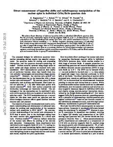
FIG. 1. 共Color兲 共a兲 A LEAP® tomographic reconstruction of an Fe-1.7 at. % Cu specimen, whose thermal history is detailed in the text. Only Cu atoms are displayed for clarity. 共b兲 The 546 precipitates are fitted as ellipsoids 共Ref. 24兲. A Delaunay mesh connects the precipitate centers. This is used to find “interacting precipitates” and to exclude the convex hull.

chosen over more efficient algorithms that calculate explicitly the distance between ellipsoids,29,30 so that it can be used with other abstractions of precipitate morphology 共such as the isoconcentration surface兲 and additional constraints 共such as calculation of interplanar edge-to-edge distances兲 and because a gratis implementation exists.31 COBYLA minimizes the distance between two points, x and y in the analysis space, 冑兺 j共x j − y j兲2. The constraints are that x and y must fall on the ellipsoid. This is simplified by the fact that applying the inverse transformation of ellipsoids transforms them back into unit spheres, centered at the origin 共so 兺 jxTj x = 1 and 兺 j y Tj y = 1, where the superscript Ti is the inverse transform of the best-fit ellipsoid for precipitate i兲. The initial guess is chosen as the two closest points that satisfy these constraints that lie on the line that connects the precipitate centers. Interprecipitate distance distributions 共IDDs兲 may be generated using different combinations of Delaunay neighbors, as in Fig. 2. An IDD is the convolution of a PSD and the centerto-center distances. In Fig. 2共a兲, an IDD for all 6671 Delaunay neighbor distances yields a mean 3D interprecipitate 3D 典, of 16 nm. Figure 2共b兲 displays two subsets distance, 具␭e-e of this IDD, each with 471 lengths because there is one distance associated with each of the 471 interior precipitates

that are not on the convex hull. The distance between nearest precipitates is often used to calculate precipitate-dislocation 3D interactions. The IDD for this is much sharper and 具␭e-e 典 = 2.6 nm. Precipitates that are very close to one another might be bypassed as a pair by a dislocation. The longest Delaunay distances provide an upper bound to the interactive distance. This is probably not physically important for plastic deformation, but may be relevant for other physical phenomena. The IDD for this case is broader, does not overlap the shortest distances, and has a mean value that is an order of 3D 典 = 25 nm兲. While 69% of the dismagnitude larger 共具␭e-e tances are shorter than this mean value, the distribution has a long tail that extends to 58 nm. Although the length of this tail is on the order of the diameter of the analysis volume, this is coincidental and it is the large variance in Delaunay distances that causes it. This tail is quite short and less than 5% of the lengths are 50 nm or longer. 3D 典 that is of interest, but In certain cases, it is not 具␭e-e 2D rather the interplanar edge-to-edge distance, 具␭e-e 典. This might, for instance, be a glide plane of a dislocation. This 2D distance can be calculated by imposing an additional constraint for COBYLA—that x and y values must fall on a par3D 2D 典 and 具␭e-e 典 can be calcuticular plane. For comparison, 具␭e-e lated from one another by assuming precipitates are distributed on a cubic lattice,2

冉冑 3

3D 具␭e−e 典=

冊

4␲ − 2 具R典, 3␾

共1兲

where ␾ is the volume fraction of precipitates. Assuming a square array of precipitates,

Downloaded 07 Jul 2007 to 129.105.215.213. Redistribution subject to AIP license or copyright, see http://apl.aip.org/apl/copyright.jsp

013111-3

Appl. Phys. Lett. 91, 013111 共2007兲

Karnesky, Isheim, and Seidman

We are in the midst of applying this approach to calculate the strength of different alloys using analytical equations.2 We are also using it to evaluate the statistical accuracy of simulated microstructures, which are used in a continuum dislocation dynamics simulation that calculates a stress-strain curve.32 This research is supported by the Office of Naval Research, under Contract No. N00014-03-1-0252. One of the authors 共R.A.K.兲 received partial support from a Walter P. Murphy Fellowship and the U.S. Department of Energy 共DEFG02-98ER45721兲. The authors thank S. K. Lahiri and M. E. Fine for providing the Fe–Cu alloy. Imago Scientific Instruments and M. K. Miller permitted one of the authors 共R.A.K.兲 to modify the source code for ENVELOPE. D. C. Dunand and J. Jerome are thanked for discussions. 1

FIG. 3. 共Color online兲 共a兲 Interplanar 共2D兲 IDDs for the data set in Fig. 1. 2D 典 = 6.2 nm. Dashed: IDD from Fig. 2共b兲 scaled Solid: IDD of slices, with 具␭e-e 2D * 2D 典 = 5.4 nm兲. 共b兲 ␭e-e is weighted toward longer distances by Eq. 共3兲 共具␭e-e 2D* . than ␭e-e

2D 具␭e−e 典=

冉冑 冊

␲ − 2 ¯R , ␾

共2兲

where the mean planar radius ¯R is equal to 共␲ / 4兲␻2具R典, with ␻2 dependent on the PSD.2 Values for ␻2 for the LSW distribution and for the case where all precipitates are the same size are given in Ref. 2. Equating the ␾s in Eqs. 共1兲 and 共2兲 2D 3D 典 and 具␭e-e 典. Solving leads to a cubic equation relating 具␭e-e 2D for 具␭e-e典: 2D 典= 具␭e−e

3D 3 ␲共− 4␻2具R典2 + 冑3␻22具R典共2具R典 + 具␭e−e 典兲 兲 . 8具R典

共3兲

In Fig. 3, the results of the two methods for extracting 2D nearest-neighbor IDDs from the 3D data set are compared. 2D is calculated directly by imposing the additional con␭e-e straint on COBYLA that the two points must lie in the same plane, which is radial to the analysis direction. The entire tip is sampled by taking 180 1° steps. This process samples the precipitates toward the center of the tip more than those toward the hull, but has fewer edge artifacts than parallel slices 2D* is calculated from what is displayed in would have. ␭e-e Fig. 2共b兲 by applying Eq. 共3兲 with 具R典 = 1.3 nm and ␻2 = 1.046 共Ref. 2兲 共the superscript ⴱ denotes this transformation兲. Despite the simple geometrical assumptions involved in deriving Eq. 共3兲, the mean values are in reasonable agree2D 典 = 6.2 nm and ment 共with the “direct” method yielding 具␭e-e 2D * with the conversion leading to 具␭e-e典 = 5.4 nm兲. Despite this similarity in the mean values, the distributions are different. The converted IDD is narrower and weighted toward shorter distances than the IDD that is directly calculated. A more complicated stereological transformation might be needed to preserve the distribtution.15 Because the LEAP tomograph gathers 3D experimental data, it allows direct measurement 2D from planar slices taken from the 3D reconstruction of ␭e-e 3D . and ␭e-e

L. M. Brown and R. K. Ham, in Strengthening Mechanisms in Crystals, edited by A. Kelly and R. B. Nicholson 共Applied Science, London, 1971兲, pp. 9–135. 2 E. Nembach, Particle Strengthening of Metals and Alloys 共Wiley-Interscience, New York, 1996兲. 3 I. M. Lifshitz and V. V. Slyozov, J. Phys. Chem. Solids 19, 35 共1961兲. 4 C. Wagner, Z. Elektrochem. 65, 581 共1961兲. 5 S. Torquato, Annu. Rev. Mater. Res. 32, 77 共2002兲. 6 J. Quintanilla, Polym. Eng. Sci. 39, 559 共2004兲. 7 B. Lu and S. Torquato, J. Chem. Phys. 98, 6472 共1993兲. 8 S. Torquato, Phys. Rev. E 51, 3170 共1995兲. 9 J. R. Macdonald, J. Phys. Chem. 96, 3861 共1996兲. 10 Z. H. Liu, Y. Li, and K. W. Kowk, Polymer 42, 2701 共2001兲. 11 A. Tewari and A. M. Gokhale, Mater. Sci. Eng., A 385, 332 共2004兲. 12 T. F. Kelly and D. J. Larson, Mater. Charact. 44, 59 共2000兲. 13 D. N. Seidman, Annu. Rev. Mater. Res. 37, 127 共2007兲. 14 J. W. Leggoe, Scr. Mater. 53, 1263 共2005兲. 15 J. Ohser and F. Mücklich, Statistical Analysis of Microstructures in Materials Science 共Wiley, New York, 2000兲. 16 S. K. Lahiri and M. E. Fine, Metall. Trans. 1, 1495 共1970兲. 17 M. E. Fine and D. Isheim, Scr. Mater. 53, 115 共2005兲. 18 J. Liu, A. van de Walle, G. Ghosh, and M. Asta, Phys. Rev. B 72, 144109 共2005兲. 19 S. R. Goodman, S. S. Brenner, and J. R. Low, Metall. Trans. 4, 2363 共1973兲. 20 M. K. Miller, K. F. Russell, P. Pareige, M. J. Starink, and R. C. Thomson, Mater. Sci. Eng., A 250, 49 共1998兲. 21 M. Murayama, Y. Katayama, and K. Hono, Metall. Mater. Trans. A 30, 345 共1999兲. 22 D. Isheim, M. S. Gagliano, M. E. Fine, and D. N. Seidman, Acta Mater. 54, 841 共2006兲. 23 D. Isheim, R. P. Kolli, M. E. Fine, and D. N. Seidman, Scr. Mater. 55, 35 共2006兲. 24 R. A. Karnesky, C. K. Sudbrack, and D. N. Seidman, Scr. Mater. 57, 353 共2007兲. 25 M. K. Miller and E. A. Kenik, Microsc. Microanal. 10, 336 共2004兲. 26 K. Clarkson, in Proceedings of the 31st IEEE Symposium on Foundations of Computer Science, Pittsburgh, PA, 1992 共unpublished兲, pp. 387–395. 27 C. B. Barber, D. P. Dobkin, and H. Huhdanpaa, ACM Trans. Math. Softw. 22, 469 共1996兲. 28 M. Powell, in Advances in Optimization and Numerical Analysis, edited by S. Gomez and J. Hennart 共Kluwer Academic, Dordrecht, 1994兲, pp. 51–67. 29 A. Lin and S.-P. Han, SIAM J. Optim. 13, 298 共2002兲. 30 K.-A. Sohn, B. Jüttler, M.-S. Kim, and W. Wang, in PG 2002, edited by S. Coquillart, H.-Y. Shum, and S.-M. Shi-Min Hu 共IEEE Computer Society, Los Alamitos, CA , 2002兲, pp. 236–245. 31 E. Jones, T. Oliphant, and P. Peterson, SCIPY, open source scientific tools for PYTHON, 2001. 32 V. Mohles, Mater. Sci. Eng., A 365, 144 共2004兲.

Downloaded 07 Jul 2007 to 129.105.215.213. Redistribution subject to AIP license or copyright, see http://apl.aip.org/apl/copyright.jsp