the simulation of IGW breaking was proposed by Fruman & Achatz (2012): First, they ..... resources were provided by the HLRS Stuttgart under the grant TIGRA.
J. Fluid Mech. (2013), vol. 720, pp. 424–436. © 2013 Cambridge University Press DOI: 10.1017/jfm.2013.108 Printed in the United Kingdom
1
Direct numerical simulation of a breaking inertia-gravity wave S. REMMLER1 , M. D. FRUMAN2
AND
S. HICKEL1
1
Institute of Aerodynamics and Fluid Mechanics, Technische Universit¨ at M¨ unchen, D-85747 Garching bei M¨ unchen, Germany 2 Institute for Atmospheric and Environmental Sciences, Goethe-Universit¨ at Frankfurt, D-60438 Frankfurt am Main, Germany (Received October 31 2012; revised February 15 2013; accepted February 19 2013.)
We performed fully resolved three-dimensional numerical simulations of a statically unstable monochromatic inertia-gravity wave using the Boussinesq equations on an f -plane with constant stratification. The chosen parameters represent a gravity wave with almost vertical direction of propagation and a wavelength of 3 km breaking in the middle atmosphere. We initialised the simulation with a statically unstable gravity wave perturbed by its leading transverse normal mode and the leading instability modes of the time-dependent wave breaking in a two-dimensional space. The wave was simulated for approximately 16 hours, which is twice the wave period. After the first breaking triggered by the imposed perturbation, two secondary breaking events are observed. Similarities and differences between the three-dimensional and previous two-dimensional solutions of the problem and effects of domain size and initial perturbations are discussed.
1. Introduction Today there is no longer any doubt that gravity waves play an important role in the global circulation in the atmosphere. Sawyer (1959) was one of the first to note the necessity of taking gravity waves into account in numerical weather forecast models. Several authors (Bretherton 1969; Lilly 1972; Blumen & McGregor 1976) attempted to quantify the gravity wave drag exerted by orographic gravity waves on the mean flow, finding values of the order of 1 Pa, which can be sufficient to accelerate the mean flow by several m/s per day (Nappo 2002). Chun & Baik (1998) found even larger values of acceleration and deceleration due to gravity waves generated by thermal forcing in cumulus convection. The direct effects of gravity waves on the general circulation in the troposphere and lower stratosphere are only minor, although gravity wave breaking can lead to clear-air turbulence and locally enhanced turbulent diffusion in this region. On the other hand, gravity waves strongly influence the circulation in the mesosphere (the altitude range between 50 and 90km), where they are responsible for the cold summer pole mesopause (Houghton 1978), and in the stratosphere, where together with other equatorial waves they lead to the quasi-biennial oscillation in equatorial winds (Dunkerton 1997a). Despite this unquestioned importance of gravity waves, their treatment in present general circulation models remains unsatisfactory. The major part of the gravity wave spectrum is not or is only marginally resolved by the numerical grids and must thus be explicitly parametrised. Various parametrisations have been proposed, e. g. by Lindzen (1981), Holton (1982) and others. Reviews of gravity wave parametrisation schemes are provided by McLandress (1998) and Fritts & Alexander (2003). Generally, the upward propagation of linear waves through the atmosphere is computed using the WentzelKramers-Brillouin-Jeffreys (WKBJ) approximation, which is based on the assumption
2
S. Remmler, M. D. Fruman and S. Hickel
of a slowly varying background flow field. During the upward propagation of the wave, the amplitude typically grows as the ambient density decreases. The wave becomes more nonlinear until it reaches the threshold of static stability (i. e. where the vertical gradient of total potential temperature becomes locally negative) and breaks. Most parametrisation schemes account for this effect by transferring some fraction of the wave momentum to the mean flow and reducing the wave amplitude accordingly. All aspects of gravity wave parametrisation, i. e. sources, propagation and breaking are associated with large uncertainties. Consequently, the schemes have to be carefully tuned in order to obtain realistic results for the general circulation. An improvement of the gravity wave parametrisation (without ad-hoc tuning) requires a better understanding of the physical process of wave breaking, which can only be obtained through a detailed analysis of breaking events. Theoretical analyses of inviscid (Mied 1976; Drazin 1977) and weakly viscous (Klostermeyer 1982) breaking gravity waves show that monochromatic high frequency gravity waves (HGWs), i. e. waves unaffected by rotation, are linearly unstable regardless of their amplitude, either through parametric subharmonic instability or convective instability. As opposed to HGWs, low frequency inertia-gravity waves (IGWs) are influenced by the Coriolis force and thus have a nonzero third velocity component perpendicular to the plane of the wave. Dunkerton (1997b) and Achatz & Schmitz (2006b) showed that this influences the orientation of the most unstable perturbations. Hence the breaking mechanism in IGWs differs fundamentally from HGWs and has to be investigated separately. The onset of gravity wave breaking, i. e. the initial growth of some instability modes, can be treated as a two-dimensional problem with three velocity components. However, the breaking process itself is inherently three-dimensional, and the breaking dynamics in two- and three-dimensional simulations strongly differ from each other, as pointed out first by Andreassen et al. (1994) and later by Fritts et al. (1994, 2009). The analysis of the breaking process of gravity waves in the atmosphere at realistic scales and Reynolds numbers requires highly resolved non-linear three-dimensional simulations. For IGWs, which are affected by rotation, no such simulations have yet been published. The high resolution simulations of Fritts et al. (2009) are restricted to HGWs, where the velocity vector of the base wave lies in the plane of the wave. Lelong & Dunkerton (1998) simulated breaking IGWs at a greatly reduced ratio of the BruntV¨ ais¨ al¨ a frequency to the Coriolis parameter compared to atmospheric values. There and in many other studies (Winters & D’Asaro 1994; Andreassen et al. 1998; D¨ornbrack 1998; Afanasyev & Peltier 2001, and others) no attempt is made to resolve all turbulence scales at realistic Reynolds numbers. Instead, either a subgrid-scale (SGS) parametrisation of turbulence or a hyperviscosity formulation is used. Alternatively, the Reynolds number is greatly reduced to match laboratory experiments. In none of the aforementioned studies have the used SGS parametrisations been validated using turbulence resolving reference simulations. Clearly, however, possible effects of the SGS parametrisation on the general breaking process can only by excluded by fully resolving all turbulence scales. Since three-dimensional simulations are computationally expensive and thus not suitable for investigating a large space of parameters, the following multi-step approach for the simulation of IGW breaking was proposed by Fruman & Achatz (2012): First, they computed the leading primary instabilities of a given IGW. Second, they performed highresolution nonlinear simulations initialised with the superposition of the IGW and its leading unstable modes. These simulations are restricted to a two-dimensional domain but contain three independent velocity components, so they are referred to as “2.5”dimensional. Next, this 2.5-dimensional time dependent flow was analysed for stability
Direct numerical simulation of a breaking inertia-gravity wave
3
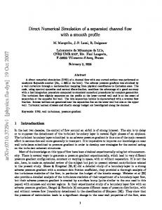
Figure 1. Left: Computational domain in the rotated coordinate system x, y, z. The earth coordinates are denoted as x0 , y 0 , z 0 . cp and cg indicate the phase and group velocity. Right: Initial condition with secondary SV perturbation. Contours of buoyancy in colours and an iso-surface at b = 0 in green.
with respect to secondary perturbations varying in the remaining spatial direction. We will now extend this procedure by adding a fourth and last step: a fully three-dimensional nonlinear integration of the breaking event. The initial condition is the same as that of the 2.5-dimensional simulations, but perturbed by the fastest growing secondary perturbation. The resulting initial flow field is then fully three-dimensional. The domain size is determined by the wavelength of the base wave and by the scales of the primary and secondary perturbations.
2. Physical and mathematical model Inertia-gravity waves have a horizontal wavelength that can easily reach some hundreds of kilometres. We can avoid simulating in such a large domain by rotating the coordinate system so that one coordinate axis is aligned with the direction of propagation of the wave. Figure 1 shows the unrotated and rotated coordinate systems for the case of a transverse primary perturbation. We obtain the wave coordinates x, y, z by rotating the earth coordinates x0 , y 0 , z 0 first by 90◦ − Θ about the y 0 axis and then by 90◦ about the z axis. Then x is the direction of the primary perturbation, y is the direction of the secondary perturbation and the base wave varies in the z direction. In this coordinate system the true vertical direction is described by the unit vector ez0 = [0, sin Θ, cos Θ]. We can write the non-dimensional Boussinesq equations on an f -plane as ∇·u=0
(2.1a) ez0 × u b 1 2 − ∇p + ez0 + ∇ u (2.1b) ∂t u + ∇ · (uu) = − Ro Re F r2 ˆ 2 u · ez0 + 1 ∇2 b, ∂t b + ∇ · (bu) = −N (2.1c) P r Re where velocities u are made non-dimensional by U, all spatial coordinates x by the length scale L, normalised pressure p by U 2 , and time t by L/U. Density deviations from the background mean are measured by the buoyancy b = (θ∗ −θ)/θ0 (θ: background potential temperature, θ∗ : local potential temperature, θ0 : reference potential temperature). The non-dimensional parameters are Ro =
U , fL
U Fr = √ , gL
Re =
UL , ν
ˆ 2 = ∂b = N 2 L , N ∂z 0 g
Pr =
ν , α
(2.2)
4
S. Remmler, M. D. Fruman and S. Hickel
where f is the Coriolis parameter, g is the gravitational acceleration, ν is the kinematic viscosity, N 2 = (g/θ0 )dθ/dz 0 is the Brunt-V¨ais¨al¨a frequency and α is the thermal diffusivity. If we use the rotated coordinates as defined above, we find that the monochromatic gravity wave is an exact solution to the Boussinesq equations 2.1: � � f /K Ω/K N 2 /K [u, v, w, b] = a cos ϕ, − sin ϕ, 0, − cos ϕ , (2.3) cos Θ sin Θ cos Θ g sin Θ where K = 2π/λ is the base wave number, ϕ = Kz − Ωt is the phase angle of the wave and the wave frequency Ω is determined by the dispersion relation Ω2 = N 2 cos2 Θ + f 2 sin2 Θ.
(2.4)
The non-dimensional wave amplitude a is defined such that the wave is statically unstable for a > 1 and statically stable for a < 1. For the detailed derivation of the wave solution in the rotated coordinate system and for the primary and secondary instability analysis, see the work of Achatz (2005, 2007) and Fruman & Achatz (2012). The flow under investigation is highly three-dimensional and thus requires appropriate definitions for quantifying turbulent mixing. Fully resolved DNS allow for a direct evaluation of the local dissipation rates εk and εp of kinetic energy 21 ui ui and available ˆ 2 F r2 from the velocity and buoyancy fields: potential energy 12 b2 /N � �� 1
∂xj ui + ∂xi uj ∂xj ui + ∂xi uj Re 1 h(∂xi b) (∂xi b)i , εp = ˆ 2 F r2 P r Re N
εk =
(2.5) (2.6)
where h...i indicates an appropriate spatial average. These definitions fully exploit the three-dimensional information available in DNS and, in particular, they do not involve any assumptions about the ratio of horizontal to vertical scales, as sorting procedures (Thorpe 1977) generally do. For a detailed analysis of the energy transfer and dissipation in a stably stratified turbulent flow we refer to Remmler & Hickel (2012b). The Boussinesq equations are discretised by a finite-volume fractional-step method on a staggered Cartesian mesh. For time advancement the explicit third-order RungeKutta scheme of Shu (1988) is used. The time-step is dynamically adapted to satisfy a Courant-Friedrichs-Lewy condition with CF L 6 1.0. The spatial discretization is based on non-dissipative central schemes with 4th order accuracy for the advective terms and 2nd order accuracy for the diffusive terms and the pressure Poisson solver. The Poisson equation for the pressure is solved at every Runge-Kutta sub step, using a direct method (based on the Fast Fourier Transform and modified wavenumbers consistent with the underlying staggered grid method) in the z direction and an iterative Stabilised BiConjugate Gradient (BiCGSTAB) solver in the x-y planes. For more details on our flow solver INCA (www.inca-cfd.org), its performance and validation for atmospheric flows we refer to Remmler & Hickel (2012a,b).
3. Test case definition We consider a statically unstable monochromatic inertia-gravity wave whose parameters are chosen such that inertial and buoyancy forces have similar magnitudes. All physical parameters are summarised in table 1. A comparable 2.5-D case was already investigated by Achatz (2007) and Fruman & Achatz (2012) at a wavelength of λ = 6 km. To reduce the necessary domain size, we repeated their analysis for a wavelength of
Direct numerical simulation of a breaking inertia-gravity wave
wavelength wave vector orientation dimensional wave amplitudes non-dimensional wave amplitude kinematic viscosity Coriolis parameter Brunt-V¨ ais¨ al¨ a frequency gravitational acceleration thermal diffusivity
λ Θ u ˆ a ν f N g α
= = = = = = = = =
3 km 89.5◦ 8.97 m/s 1.2 1 m2 /s 1.367 · 10−4 s−1 0.02 s−1 9.81 m/s2 1 m2 /s
horizontal wavelength (downward) phase velocity wave oscillation period
λx0 = 343 km cp = 0.106 m/s T = 7.87 h
5
; vˆ
= 14.56 m/s ; ˆb = 0.0234
; ; ; ; ;
= = = = =
Re Ro ˆ N Fr Pr
43665 35.5 6.12 0.0848 1
Table 1. Physical parameters of the investigated inertia-gravity wave. The non-dimensional numbers were computed based on the wavelength L = λ = 3 km and the maximum velocity U = vˆ = 14.56 m/s.
only λ = 3 km and found that the wavelengths of the perturbations scale with the base wavelength without changing the general character of the breaking event. The kinematic viscosity used here and in the preceding 2.5-D studies corresponds to a geopotential altitude of 81 km in the US Standard Atmosphere, which is in the upper part of the range where gravity wave breaking occurs and affects the middle-atmosphere circulation. We refrain from using a lower kinematic viscosity (corresponding to lower altitudes) to limit the computational costs and to keep our results comparable to the previous work. The base wave as described by equation 2.3 is initially disturbed by its leading transverse normal mode (Achatz 2007), which has a wavelength of 3891 m. This wavelength determines the domain size in the x direction. The perturbed wave field is further perturbed by the fastest growing singular vector (SV) of the equations 2.1 linearised about the time dependent nonlinear 2.5-D solution (Fruman & Achatz 2012). This singular vector has a wavelength of 400 m, which determines the domain size in the y direction. The amplitude of the SV perturbation is somewhat arbitrary. We chose the amplitude such that the maximum energy density in the SV is 1% of the maximum initial energy density in the wave and primary normal mode. The initial condition is displayed in figure 1. The domain size for the simulations presented here was 3981 m × 400 m × 3000 m. We conducted two simulations on different grids: a fine simulation designed to fully resolve all turbulence scales and a second, coarser simulation at approximately half the resolution. The grid of the fine simulation had 1350 × 128 × 1000 cells, which corresponds to a uniform cell size ∆ ≈ 3 m in all directions. The coarse grid had a resolution of ∆ ≈ 6 m (640 × 64 × 500). The governing equations were integrated in time for 34000 s (fine) and 60000 s (coarse).
4. Results and discussion −1/4
We verified the chosen grid resolution by computing the Kolmogorov length η = ν 3/4 εk with the maximum of the kinetic energy dissipation rate in the domain, see figure 2(a). According to Yamazaki et al. (2002), the low-order statistics of turbulence are basically unaffected by the resolution as long as kmax η & 1, i. e. ∆ < πη. By this criterion, we find that the fine simulation is fully resolved and the coarse simulation is insufficiently resolved. Nevertheless, the coarse simulation remains free of unphysical oscillations with-
6
S. Remmler, M. D. Fruman and S. Hickel 5
(a)
1.3 3-D DNS (1350 x 128 x 1000) 3-D DNS (640 x 64 x 500)
4.5
-2
(b)
10 1.2
4 3.5
1
2 1.5
amplitude
10-4
0.9
1
εt [W/kg]
-3
10
2.5
a
η [m]
dissipation
1.1
3
0.5 0.8
0 0
10000
20000 t [s]
30000
40000
0
10000
20000 t [s]
30000
40000
Figure 2. Time series for (a) Kolmogorov length and (b) nondimensional amplitude of the primary wave and total energy dissipation. Solid lines: full resolution 3-D DNS; dashed lines: half resolution 3-D DNS; symbols: 2.5-D DNS; dash-dotted lines: laminar decay. εt εk εp
(a) 10-2
(b)
0.5
Γ = εp / εk
ε [W/kg]
0.4
10-3
0.3
0.2
0.1 3-D DNS (1350 x 128 x 1000) 3-D DNS (640 x 64 x 500)
-4
10
0 0
10000
20000 t [s]
30000
40000
0
10000
20000 t [s]
30000
40000
Figure 3. Spatial mean values of energy dissipation: (a) contributions to the energy dissipation for the fine grid, (b) Γ = εp /εk in coarse and fine simulation.
out requiring any artificial numerical dissipation, which we attribute to the good spectral resolution properties (modified wavenumber) of staggered-grid methods. The most important quantities extracted from the simulations are the amplitude of the primary wave and the spatially averaged energy dissipation rate, shown in figure 2(b). For 2 comparison, we added the curves for a purely laminar wave decaying like a(t) = a0 e−νK t with the parameter a0 fitted to match the final (laminar) state of the original wave. During the first wave period (T = 28342 s), there are three distinct occurrences of wave breaking characterised by a rapid decrease of the wave amplitude and a strongly increased total dissipation rate. After t = 35000 s the wave has become laminar and no longer shows signs of turbulence and enhanced dissipation. Both 3-D simulations predict basically the same temporal development of the amplitude. There are some differences in the dissipation rate between the fine and coarse simulations, especially during the second and third breaking events. However, the overall agreement between the two simulations is very good. This indicates that the full resolution simulation yields a grid-converged solution. We compare the 3-D DNS to a 2.5-D simulation performed with the model of Achatz (2007) initialised with just the IGW and the leading transverse normal mode. The wave amplitude from the 2.5-D simulation with ∆ ≈ 3 m is also plotted in figure 2(b). While the temporal evolution of the wave amplitude is not exactly the same in the 2.5-D and
Direct numerical simulation of a breaking inertia-gravity wave
(a) Ri
(b) εk
7
(c) εp
Figure 4. Hovm¨ oller plots of Richardson number (a) and energy dissipation (b and c). The dashed lines indicate a fixed position in space while the coordinate system is moving downward with the phase speed of the wave.
3-D simulations, the duration of the breaking event and the total energy decrease due to the breaking are similar. Details, such as the secondary breaking events observed in the 3-D simulations are not reproduced by the 2.5-D simulation and the breaking lasts longer in the 3-D simulations. We decomposed the energy dissipation into kinetic εk and potential energy dissipation εp in figure 3(a). Both show peaks during the three breaking events, but the peaks of εk are much more pronounced, so that the ratio Γ = εp /εk is temporally reduced during these events (figure 3(b)). The strongest reduction is observed during the third event. This means that the energy dissipation is caused by strong gradients in the velocity field rather than the buoyancy field during this event. The dissipation rates averaged in the x-y plane (perpendicular to the wave vector) are plotted against time in figure 4. The coordinate system is moving with the phase speed of the primary wave, so the most unstable region is always in the upper half of the domain and the most stable part in the lower half. An indicator for stability is the Richardson number ˆ 2 + hP ∂x b ez0 ,i i ˆ 2 + h∂z0 bi N N i i D E= � Ri = (4.1) �P �2 � , 2 2 P 2 0 0 0 F r (∂z0 u ) + (∂z0 v ) 2 0 Fr k j ∂xk uh,j ez ,k where u0h,j = uj − (u · ez0 )ez0 ,j is the horizontal velocity in the earth frame and h...i indicates an average in the x-y plane. The Richardson number is shown in figure 4(a). Blue regions indicate static instability, because the Richardson number is negative there. Violet regions correspond to 0 < Ri < 0.25 and hence dynamic instability. Comparison of figures 4(a) and 4(b) shows that turbulent dissipation of kinetic energy is spatially and temporally correlated with static and dynamic instability of the mean state. Note that this is an average Richardson number in the x-y-plane, so locally the value of Ri can strongly differ from this average. The first breaking event triggered by the initial perturbation is spread over the whole domain. Turbulence (indicated by enhanced kinetic energy dissipation, figure 4(b)) is generated in the stable and unstable regions of the wave, but only in the stable region does this lead to strong potential energy dissipation, see figure 4(c). Both secondary breaking events (around t = 12000 s and t = 16000 s) have hardly any signature in εp . Most energy is dissipated mechanically in the unstable half of the domain. Figure 5 shows some snapshots of the wave field during the first breaking event. The
8
S. Remmler, M. D. Fruman and S. Hickel
(a) t = 0 s
(b) t = 280 s
(c) t = 520 s
(d) t = 1055 s
(e) t = 1570 s
(f) t = 2000 s
Figure 5. Temporal evolution of the first breaking event. Background: plane at y = 400 m coloured by buoyancy; foreground: iso-surface of Q = 0.004 s−2 , indicating turbulent vortices.
(a) t = 12680 s
(b) t = 13100 s
(c) t = 13560 s
Figure 6. Temporal evolution of the second breaking event. Colouring as in figure 5.
(a) t = 16110 s
(b) t = 16650 s
(c) t = 17110 s
Figure 7. Temporal evolution of the third breaking event. Colouring as in figure 5.
� � yellow iso-surface of Q = 12 |Ω|2 − |S|2 = 18 |∂xj ui − ∂xi uj |2 − |∂xj ui + ∂xi uj |2 is used to visualise turbulent vortices. During the first 1000 s strongly three-dimensional turbulence structures develop in the unstable half. The strong perturbations of the isopycnals quickly vanish. In the meantime a strong two-dimensional overturning develops in the stable region, eventually breaking and generating three-dimensional turbulence around t = 1500 s. While turbulence is sustained for a long time in the unstable half of the wave, it decays quickly through the damping effect of stratification in the stable half. In the 2.5-D simulations, the turbulence in the stable half of the wave is much longer lived. Achatz & Schmitz (2006a) and Achatz (2007) attribute this turbulence to small scale waves excited near the level of maximum static instability encountering a critical level associated with the zero in the v component of the original wave. This effect appears to be less important in 3D.
Direct numerical simulation of a breaking inertia-gravity wave
1.2
dissipation
amplitude
1.15
10-3
1
10-4
0.9
(b) 1.2
a
1.1
1.25
10-2
0.8
a
Ly = 400m, SV Ly = 400m, noise Ly = 200m, noise Ly = 800m, noise
εt [W/kg]
1.3
(a)
9
1.1
1.05
1
0
10000
20000 t [s]
30000
40000
0
2500
5000
t [s]
Figure 8. Time series for the non-dimensional amplitude of the primary wave and total energy dissipation for different secondary perturbations and domain sizes. (a) full time range, (b) amplitude during the first 5000 s (circles: 2.5-D simulation)
The second breaking event (figure 6) is much weaker than the first. It is initiated by a growing instability of the large-scale wave that spans both the statically stable and unstable regions. Note that the nondimensional amplitude of the wave drops below the threshold of static instability right before the event becomes visible. Unlike the first event, the instability is too weak to generate turbulence in the stable region, but some turbulence appears in the unstable region. The third breaking event (figure 7) is stronger than the second, but still much weaker than the first. It is not preceded by a visible instability of the primary wave. The isopycnals in figure 7(a) are almost perfectly horizontal. The turbulence emerges “out of nothing” in the unstable region, causes some mixing there and eventually decays. An explanation can be found in figure 4(b). By the time of the third breaking event, the primary wave has propagated about half a wavelength downwards, so the unstable region of the wave has arrived at the fixed point in space where the wave was most stable at the beginning of the simulation. There seems to be some “leftover” turbulence generated by the first breaking, which is amplified as soon as the stability in this region has decreased sufficiently. Therefore, the third event is not really a third breaking event, but rather a burst of turbulence triggered by the arrival of the dynamically unstable part of the wave in a region preconditioned by the first breaking event. In order to investigate the effect of the particular choice of secondary perturbation on the three-dimensionalisation and overall evolution of the flow, we conducted additional simulations at the 6 m resolution with the SV perturbation replaced by low level white noise and with the domain size Ly in the direction of the secondary perturbation varied between 200 m and 800 m. Since white noise is a superposition of perturbations with all possible scales, it also contains contributions of the SV that leads to maximum energy growth, as long as the domain size is large enough. For Ly = 400 m and Ly = 800 m, the wave amplitude decay and energy dissipation are similar to those of the SV initialization, but for the smaller domain size the initial peak of the dissipation rate is smaller and the second and third breaking events are missing completely, see figure 8(a). A close look at the first hour of the integrations in figure 8(b) reveals that the quick threedimensionalisation seen in the SV simulation occurs only in the simulation with Ly = 800 m, while the other two white noise simulations follow the 2.5-D solution, and threedimensional effects take longer to emerge. This reassures us that the SV is physically
10
S. Remmler, M. D. Fruman and S. Hickel
meaningful and representative of the perturbations that grow spontaneously even in a larger domain with many more degrees of freedom.
5. Conclusion We have presented the first turbulence resolving three-dimensional simulations of an inertia-gravity wave breaking under environmental conditions realistic for the middle atmosphere. The breaking was stimulated by optimal perturbations of the wave derived from linear theory. The primary breaking of the unstable wave stretches over the complete space of the wave and is responsible for a strong reduction of the wave amplitude by more than 12% within less than 10000 s (on the order of half a wave period). A pure laminar decay of the wave would take three times as long for the same amplitude reduction. We observed a second and a third burst of turbulence after the first breaking event. During these secondary events turbulence appears only in the unstable region of the wave and most energy is dissipated mechanically rather than thermally. The second event is negligible with regard to its reduction of the amplitude of the primary wave. It is preceded by a weak instability of the wave, which has an amplitude close to the threshold of static instability at that time. During the third event the reduction of the primary wave amplitude is more severe, amounting to about 5% of the amplitude. However, the third event is not really a breaking event, but rather a burst of turbulence in the unstable region of the wave triggered by disturbances created during the first breaking of the wave. As previous simulations of breaking IGWs employed a 2.5-D approximation, i.e. a twodimensional domain and three velocity components, we conducted a 2.5-D simulation of the same wave breaking case to investigate the effects of three-dimensionality. Details such as the secondary breaking events observed in the 3-D DNS are not reproduced by the 2.5-D simulation and the breaking lasts longer in the 3-D simulations. However, the overall results in terms of total amplitude reduction and breaking duration are similar between the 3-D and 2.5-D simulations. This similarity is important to note, since the singular vector analysis that we used to determine the domain size for the 3-D DNS was based on the 2.5-D simulation. DNS where we replaced the secondary SV perturbation by white noise and varied the domain size, showed that a SV initialization is both physically meaningful and efficient, as it leads to a realistic three-dimensionalisation of the flow in the smallest possible domain. With these first fully resolved three-dimensional direct numerical simulations of a breaking IGW we hope to present a valuable reference case for testing and validation of models involving less brute-force resolution and more physics-based parameterisation. This may include large eddy simulations as well as more abstract methods like WKBJ models, which can lead to efficient and more reliable representation of gravity waves in atmospheric circulation models. We gratefully acknowledge the support of Ulrich Achatz, who was the scientific spiritus rector of the project. This work was funded by the German Research Foundation (DFG) under the grant HI 1273-1 and the MetStr¨om priority programme (SPP 1276). Computational resources were provided by the HLRS Stuttgart under the grant TIGRA.
REFERENCES
Direct numerical simulation of a breaking inertia-gravity wave
11
Achatz, U. 2005 On the role of optimal perturbations in the instability of monochromatic gravity waves. Phys. Fluids 17 (9), 094107. Achatz, U. 2007 The primary nonlinear dynamics of modal and nonmodal perturbations of monochromatic inertia gravity waves. J. Atmos. Sci. 64, 74. Achatz, U. & Schmitz, G. 2006a Optimal growth in inertia-gravity wave packets: Energetics, long-term development, and three-dimensional structure. J. Atmos. Sci. 63, 414–434. Achatz, U. & Schmitz, G. 2006b Shear and static instability of inertia-gravity wave packets: Short-term modal and nonmodal growth. J. Atmos. Sci. 63, 397–413. Afanasyev, Y. D. & Peltier, W. R. 2001 Numerical simulations of internal gravity wave breaking in the middle atmosphere: The influence of dispersion and threedimensionalization. J. Atmos. Sci. 58, 132–153. Andreassen, Ø., Øyvind Hvidsten, P., Fritts, D. C. & Arendt, S. 1998 Vorticity dynamics in a breaking internal gravity wave. Part 1. Initial instability evolution. J. Fluid Mech. 367, 27–46. Andreassen, Ø., Wasberg, C. E., Fritts, D. C. & Isler, J. R. 1994 Gravity wave breaking in two and three dimensions 1. Model description and comparison of two-dimensional evolutions. J. Geophys. Res. 99, 8095–8108. Blumen, W. & McGregor, C. D. 1976 Wave drag by three-dimensional mountain lee-waves in nonplanar shear flow. Tellus 28 (4), 287–298. Bretherton, F. P. 1969 Waves and turbulence in stably stratified fluids. Radio Sci. 4 (12), 12791287. Chun, H.-Y. & Baik, J.-J. 1998 Momentum flux by thermally induced internal gravity waves and its approximation for large-scale models. J. Atmos. Sci. 55, 3299–3310. ¨ rnbrack, A. 1998 Turbulent mixing by breaking gravity waves. J. Fluid Mech. 375, 113–141. Do Drazin, P. G. 1977 On the instability of an internal gravity wave. Proc. Roy. Soc. London A 356 (1686), 411–432. Dunkerton, T. J. 1997a The role of gravity waves in the quasi-biennial oscillation. J. Geophys. Res. 102, 26053–26076. Dunkerton, T. J. 1997b Shear instability of internal inertia-gravity waves. J. Atmos. Sci. 54, 1628–1641. Fritts, D. C. & Alexander, M. J. 2003 Gravity wave dynamics and effects in the middle atmosphere. Rev. Geophys. 41, 1003. Fritts, D. C., Isler, J. R. & Andreassen, Ø. 1994 Gravity wave breaking in two and three dimensions 2. Three-dimensional evolution and instability structure. J. Geophys. Res. 99, 8109–8124. Fritts, D. C., Wang, L., Werne, J., Lund, T. & Wan, K. 2009 Gravity wave instability dynamics at high reynolds numbers. Parts I and II. J. Atmos. Sci. 66 (5), 1126–1171. Fruman, M. D. & Achatz, U. 2012 Secondary instabilities in breaking inertia-gravity waves. J. Atmos. Sci. 69, 303–322. Holton, J. R. 1982 The role of gravity wave induced drag and diffusion in the momentum budget of the mesosphere. J. Atmos. Sci. 39, 791–799. Houghton, J. T. 1978 The stratosphere and mesosphere. Quart. J. Roy. Meteor. Soc. 104 (439), 1–29. Klostermeyer, J. 1982 On parametric instabilities of finite-amplitude internal gravity waves. J. Fluid Mech. 119, 367–377. Lelong, M.-P. & Dunkerton, T. J. 1998 Inertia-gravity wave breaking in three dimensions. Parts I and II. J. Atmos. Sci. 55, 2473–2501. Lilly, D. K. 1972 Wave momentum flux - A GARP problem. Bull. Am. Meteor. Soc. 53, 17–23. Lindzen, R. S. 1981 Turbulence and stress owing to gravity wave and tidal breakdown. J. Geophys. Res. 86, 9707–9714. McLandress, C. 1998 On the importance of gravity waves in the middle atmosphere and their parameterization in general circulation models. J. Atmos. Sol.-Terr. Phy. 60 (14), 1357 – 1383. Mied, R. P. 1976 The occurrence of parametric instabilities in finite-amplitude internal gravity waves. J. Fluid Mech. 78 (4), 763–784. Nappo, C. J. 2002 An introduction to atmospheric gravity waves. Academic Press.
12
S. Remmler, M. D. Fruman and S. Hickel
Remmler, S. & Hickel, S. 2012a Direct and large eddy simulation of stratified turbulence. Int. J. Heat Fluid Flow 35, 13–24. Remmler, S. & Hickel, S. 2012b Spectral structure of stratified turbulence: Direct numerical simulations and predictions by large eddy simulation. Theor. Comput. Fluid Dyn. Published online: DOI 10.1007/s00162-012-0259-9. Sawyer, J. S. 1959 The introduction of the effects of topography into methods of numerical forecasting. Quart. J. Roy. Meteor. Soc. 85 (363), 31–43. Shu, C.-W. 1988 Total-variation-diminishing time discretizations. SIAM J. Sci. Stat. Comput. 9(6), 1073–1084. Thorpe, S. A. 1977 Turbulence and mixing in a scottish loch. Philos. Trans. Roy. Soc. London A 286 (1334), pp. 125–181. Winters, K. B. & D’Asaro, E. A. 1994 Three-dimensional wave instability near a critical level. J. Fluid Mech. 272, 255–284. Yamazaki, Y., Ishihara, T. & Kaneda, Y. 2002 Effects of wavenumber truncation on highresolution direct numerical simulation of turbulence. J. Phys. Soc. Jpn. 71, 777.