Direct Numerical Simulation of Separated Low-Reynolds Number ...

Direct Numerical Simulation of Separated Low-Reynolds Number Flows around an Eppler 387 Airfoil Mehmet SAHIN, Jeremiah HALL, Kamran MOHSENI Department of Aerospace Engineering Sciences, University of Colorado at Boulder, Boulder, Colorado, 80309, USA

Koen HILLEWAERT CENAERO, Rue des Fr`eres Wright 29, B-6041 Gosselies, BELGIUM Abstract Low Reynolds number aerodynamics is important for various applications including micro-aerial vehicles, sailplanes, leading edge control devices, high-altitude unmanned vehicles, wind turbines and propellers. These flows are generally characterized by the presence of laminar separation bubbles. These bubbles are generally unsteady and have a significant effect on the overall resulting aerodynamic forces. In this study, the time-dependent unsteady calculations of low Reynolds number flows are carried out over an Eppler 387 airfoil in both two- and three-dimensions. Various instantaneous and time-averaged aerodynamic parameters including pressure, lift and drag coefficients are calculated in each case and compared with the available experimental data. An observed anomaly in the pressure coefficient around the location of the separation bubble in two-dimensional simulations is attributed to the lack of spanwise flow due to three-dimensional instabilities.

Keywords: Low Reynolds number aerodynamics, Laminar separation bubble, Direct numerical simulations, Unstructured methods, Parallel computing.

1

INTRODUCTION

Low Reynolds number aerodynamics is important for various applications including micro-aerial vehicles, sailplanes, leading edge control devices, high-altitude unmanned vehicles, wind turbines and propellers. Different from the familiar high Reynolds number aerodynamics, the low Reynolds number airfoil aerodynamics is generally characterized by the existence of the laminar separation bubbles shown in Fig. 1 which involve the separation of the laminar boundary layer from the surface due to a strong adverse 1

pressure gradient and the reattachment of the shear layer shortly downstream. The region between the separation and the reattachment point is called the separation bubble. These bubbles are generally unsteady and have a significant effect on the overall resulting aerodynamic forces. In particular they are responsible from the increase in pressure drag due to significant increase in boundary layer thickness over the separation bubble. Extensive experimental studies have been conducted in order to determine the performance characteristics of airfoils at low Reynolds numbers. McGhee et al. [14] conducted wind-tunnel experiments in the Langley Low-Turbulence Pressure Tunnel (LTPT) in order to determine the performance characteristics of the Eppler 387 airfoil at Reynolds numbers from 60,000 to 460,000. The authors computed lift and pitching moment data from the airfoil surface pressure distributions and drag data from wake surveys. Oil flow visulization was also used to determine laminar-separation and turbulent-reattachment locations. Cole and Mueller [2] performed similar experiments on the Eppler 387 airfoil and gave pressure distributions similar to that of McGhee et al. Selig and McGranahan [18] documented the aerodynamic characteristics of six different airfoils at Reynolds numbers of 100,000, 200,000, 350,000 and 500,000 including the Eppler 387 airfoil. The data taken on the E387 was compared with results from NASA Langley in the Low-Turbulence Pressure Tunnel for surface oil flow visualization, lift data, moment data and drag polars. Burgmann et al. [1] used scanning PIV measurement technique to investigate the spanwise structure and dynamics of the roll-up of vortices within the separation bubble over an SD7003 airfoil at Reynolds numbers of 20,000-60,000. The authors reported non-regular “half-moon” shaped vortices which extend in the spanwise direction. Montelpare and Ricci [15] analyzed the separation of the laminar boundary layer over the Eppler 387 airfoil at low Reynolds numbers by means of infrared thermography. Various computational approaches have been explored for the prediction of low-Reynolds number aerodynamics including inviscid potential flow simulations with viscous boundary layer corrections, ReynoldsAveraged Navier-Stokes (RANS) simulations, Large Eddy Simulations (LES) and Direct Numerical Simulations (DNS). Eppler and Somers [5] developed an airfoil analysis code based on the solution of inviscid potential flow combined with the integral boundary layer method. Pauley et al. [16] and Lin and Pauley [11] investigated the unsteady laminar boundary layer separation from an Eppler 387 airfoil at low Reynolds numbers using two-dimensional direct numerical simulations. For a relatively mild pressure gradient they found a closed steady separation bubble. When a stronger pressure gradient was applied, a limit cycle oscillations formed in which periodic vortex shedding occurred due to Kelvin-Helmholtz instabilities in the shear layer. The Strouhal number was determined by inviscid linear stability analysis to be the most amplified instability wave of the shear layer. Their computed time-average pressure coefficient distribution showed a region of nearly constant pressure followed by an abrupt decrease in surface pres-

2

sure just before reattachment. Tang [19] used RANS simulations to predict low Reynolds number airfoil aerodynamics. In order to predict the transition point, the author first performed a laminar Navier-Stokes computation and based on this laminar solution, the separation induced transition is determined as the point where the tangential velocity adjacent to the solid surface reverses its direction for the second time after the laminar separation. Then a RANS computation is performed with zero production term in the selected turbulence model before the transition point. Tatineni and Zhong [20] and Windte et al. [21] also considered the numerical simulation of low Reynolds number compressible flows over airfoils by solving RANS equations. Yuan et al. [22] conducted a parametric study of LES at a Reynolds number of 60,000 for the flow past an SD7003 airfoil. The authors investigated the effects of grid resolution and sub-grid scale models. Jovicic and Breuer [10] employed large eddy simulations applying the dynamic model by Germano as a subgrid scales model in order to predict and analyze the turbulent flow past a NACA4415 airfoil at high angle of attacks. Hoarau et al. [8] investigated the three-dimensional transition to turbulence around a NACA0012 wing at Reynolds numbers from 800 to 10,000. The authors presented three-dimensional undulated large-scale vortices row with a regular spanwise wavelength which is very similar to that of bluff body wakes. Deng [4] conducted direct numerical simulations for flow separation and transition around a NACA0012 airfoil with an attack angle of 4◦ and a Reynolds number of 100,000 and the details of flow separation, formation of detached shear layer, Kelvin-Helmholtz instability, vortex shedding, interaction of non-linear waves, breakdown and reattachment investigated. In the current paper, time-dependent both two- and three-dimensional direct numerical simulations are carried out in order the investigate the flow structure around an Eppler 387 airfoil at a Reynolds number of 60,000. There are two reasons to chose the Eppler 387 airfoil. The first one is that it reveals relatively larger laminar separation bubble at low Reynolds numbers. The second one is the availability of detailed experimental measurements. The flow structure is examined using instantaneous and mean vorticity contours as well as surface pressure and skin friction plots. The initial two-dimensional timeaverage pressure coefficient distribution indicates a region of nearly constant pressure followed by an abrupt decrease in the surface pressure just before reattachment as in the work of Pauley et al. [16]. However, three-dimensional simulations indicate significant decrease in the size of the abrupt decrease in the surface pressure which is in accord with the experimental result of McGhee et al. [14]. In our opinion this may be attributed to the importance of the spanwise flow and vorticity destruction induced by three-dimensional instabilities. The three-dimensional simulations seem to confirm the formation of “half-moon” type vortices from the laminar shear layer with no regular spanwise structure as observed experimentally of Burgmann et al. [1]. These vortices interact with each other and have tendency to burst in to the outer flow causing a significant fluid motion from airfoil surface into the mean flow.

3

The paper is organized as follows: In Section 2 the computational technique employed in the present work is briefly described. In Section 3 both two- and three-dimensional simulations are presented for the Eppler 387 airfoil at a Reynolds number of 60,000. The emphasis given to the detailed comparison of flow structure between two- and three-dimensional simulations. Conclusions are presented in Section 4.

2

NUMERICAL ALGORITHM

The numerical simulations are performed using the ARGO code [7] developed at CENAERO. The ARGO code is based on edge-based hybrid finite element- finite volume defined on unstructured P1 tetrahedral meshes. The original finite element formulation is reformulated into a finite volume formulation for computational efficiency and to allow for convective stability enhancements. In accordance to the finite element discretisation, the convective terms use central, kinetic-energy preserving flux functions; however this flux is blended with a small amount (typically 5%) of a velocity-based upwind flux for stability; the diffusive fluxes and source terms retain the original finite element formulation at all times. The time integration method is the three-point backward difference scheme. Since the numerical schemes are implicit, the flow solver must solve at each time-step a system of nonlinear equations. For this purpose, it relies on an damped inexact Newton method; the resulting linear equations are solved iteratively with the matrix-free (finite difference) GMRES algorithm, preconditioned by the minimum overlap RAS (restricted additive Schwarz) domain decomposition method [3]. The solver uses the AOMD (Algorithm Oriented Mesh Database) library [17] for the management of the topological mesh entities across the processors. In addition, it relies on the message passing interface (MPI) for exchanging data between the nodes and the Autopack library [13] for handling non-deterministic asynchronous parallel communications.

3

NUMERICAL RESULTS

In this section two- and three-dimensional time-dependent direct numerical simulations are carried out for the Eppler 387 airfoil at a Reynolds number of 60,000 and an angle of attack 6◦ . For the present calculations the relative residual is set to 10−8 . The calculations have been performed on an IBM SMP Cluster available at NCAR and Phantom Linux Cluster in the author’s group at CU.

3.1

Two-Dimensional Simulations

Initial two-dimensional calculations are carried out for the assessment of solution accuracy as well as the code validation. The computation domain far field is set to 20c where c is the cord length. In order to

4

investigate the mesh dependency of the solutions, three different meshes are employed: a coarse mesh M1 with 168,942 vertices, a medium size mesh M2 with 336,603 vertices and a fine mesh M3 with 664,824 √ vertices. The successive meshes are generated by multiplying the mesh sizes by 1/ 2 in each direction; details of the meshes are given in Table I. These successive mesh refinements are also used to adapt the both two- and three-dimensional meshes in order to reduce the computational cost. The computational coarse mesh M1 is shown in Fig. 2. The dark band near the airfoil surface is caused by boundary layer elements, which is formed in 17 layers with an initial layer thickness of 1.4c × 10−4 and a total thickness of 0.025c. The boundary layer elements continues smoothly into the wake region in order to capture the vortex shedding process. Near the airfoil leading edge the mesh along the airfoil surface is refined due to strong changes in the airfoil leading edge curvature. Refinement is also applied the outside the boundary layer so that the element sizes matches better with the elements at the far field. The meshes are partitioned into 16 sub-domains apriori for parallel computation. The calculations are carried out at a chord-based Reynolds number of 60,000 and an angle of attack 6◦ similar to that of Ref. [6]. The speed of the free stream velocity is set to 24.9m/s; the constant viscosity is modified in order to achieve the above Reynolds number. The pressure and the temperature are also set consistent with air at standard pressure and temperature. In order to speed up the calculations the energy equation is set to isothermal flow. In addition, large time steps are used during the initial calculations in order to reach vortex shedding regime with less number of iterations. Then the calculations are continued with a time step of 10−4 s. The computed time-averaged pressure distribution is given in Fig. 3. The computed results indicate convergence towards the mesh independent results. The results on meshes M2 and M3 are relatively very close to each other. Although the calculations on fine mesh M3 are desirable due to its higher accuracy, its computational cost is significantly higher particularly for the three-dimensional computations. Therefore, based on the numerical results on meshes M1 to M3 we made one more mesh adaptation in order to reduce the required number of vertices further. This adaptation level leads to a new adaptive mesh with 392,250 vertices. The results obtained on this adaptive mesh are very close to the results on the fine mesh M3 as seen in Fig. 3. Therefore, we will continue our calculations with the new adaptive mesh since the numerical results between the new adaptive mesh and the fine mesh M3 are almost identical, but with approximately half the computational cost. The time variation of lift and drag coefficients is given in Fig. 4 on the adaptive mesh for the above flow parameters. An approximate period of T = 0.0152s is observed in the lift and drag coefficients. The flow parameters are non-dimensionalized by the airfoil chord length c and the free-stream velocity U∞ . The non-dimensional Strouhal number St = c/T U∞ is 2.64 with a non-dimensional mean lift coefficient of 0.9752 and a drag coefficient of 0.0425. Several snapshot of vortex shedding at times t = 0, t = T /4,

5

t = 2T /4 and t = 3T /4 are presented in Fig. 5. In addition, airfoil surface pressure coefficient and skin friction coefficient are also given for the same time levels in Fig. 6. The vorticity contours indicate separation of the shear layer over the airfoil upper surface, after which Kelvin-Helmholtz type instabilities develop into vortices. Fig. 5 shows two large vortices over the airfoil upper surface which enlarge in size by absorbing vorticity from the shear layer. This process continues until the downstream vortex reaches a critical size. When the downstream primary vortex reaches its critical size, it begins to advect towards the trailing edge. The strengthening of the upstream vortex is observed by deepening in the Cp and Cf curves while the the strength of the convected vortex is gradually weakened. In addition to these large vortices, other small size vortices may be observed next to the airfoil surface due to vortex solid-wall interactions. The location of the large vortices and their transportation can be observed more clearly from the pressure coefficient distribution in Fig. 6 by the dip in the Cp curves. As the primary vortex leaves the trailing edge of the airfoil, a secondary vortex is formed on the lower part of the airfoil and orbit around the more stronger primary vortex once they clear the airfoil. During this motion the weaker vortex is stretched around the primary vortex and it loses its strength rapidly due to vortex stretching. In addition, the shedding of the primary vortex over the airfoil surface significantly reduces the bound vortcity of the airfoil and causes a temporary drop in the lift coefficient. The time averaged vorticity contours, pressure contours and streamlines are given in Fig. 7 around the Eppler 387 airfoil. The streamlines indicate a relatively larger separation bubble over the airfoil upper surface. A small secondary bubble is also observed beneath the primary separation bubble. The separation points may be identified more clearly from the time mean skin friction coefficient in Fig. 8. The separation point is also revealed by a start of plateau in the pressure coefficient distribution and the reattachment is indicated by the end of bump. The plateau corresponds the stable part of the separated laminar shear layer. The bump in the time averaged pressure curve is related to where the vortices spend the most time as they develop at the end of laminar separation layer. The positive spike in average skin friction coefficient around x = 0.6c is due to secondary vortices. The separation bubble causes negative skin friction over the upper surface of the airfoil which reduces the skin friction drag. However, the bump observed in the pressure coefficient causes significant pressure drag and it is significantly larger than the skin friction reduction. The comparison of the present two-dimensional numerical results with the experimental results of McGhee et al. [14] in Fig. 8 indicates significant discrepancies particularly for the pressure coefficient distribution. The values of the pressure distribution seem to be significantly off by a constant factor up to the the bump at the end of the pressure plateau. In addition, the bump almost disappears in the experimental results. As described in the following section, we believe three-dimensional effects are

6

responsible for that.

3.2

Three-Dimensional Simulations

Three-dimensional numerical simulations are carried out for the same flow parameters. The computational mesh is created by sweeping the two-dimensional cross-section of the adaptive mesh in the third dimension with 65 uniform node points between 0.0 ≤ z/c ≤ 0.5. The periodic boundary conditions are applied at z/c = 0 and z/c = 0.5 planes. The three-dimensional adapted mesh consists of 8,498,750 vertices and it is partitioned into 360 sub-domains apriori. Therefore, each processor reads its own mesh data belongs to its sub-domain number when the calculations start. Each iteration on 360 nodes at the NCAR Bluevista machine takes approximately 120 seconds. For the present three-dimensional calculations we use 2000 iterations in order to obtain the time-averaged statistics after initial transient calculations. The three-dimensional numerical results are neither as well organized nor as periodic as in two dimensions. This may be clearly seen from the lift and drag coefficient history shown in Fig. 9. There is no repeated pattern in either Cl or Cd . The time average lift and drag coefficients are computed as 0.8128 and 0.0772, respectively. Although the lift coefficient is 17% lower compared to the two-dimensional simulations the drag coefficient is approximately 82% larger. The sequence of snapshots for the vorticity magnitude iso-surfaces around an Eppler 387 airfoil is shown in Fig. 10 at several time levels along with the vorticity magnitude contours at z/c = 0.25 plane in Fig. 11. The stable laminar shear layer detaches from the airfoil upper surface due to adverse pressure gradient and Kelvin-Helmholtz instabilities grow in the separated shear layer. These instabilities in the shear layer lead to formation of rather short curved vortex tubes in the spanwise direction with no regular structure. These vortex structures are similar to the “half-moon” type vortices observed in the experimental work of Burgmann et al. [1]. Further downstream, these vortices create more complex three-dimensional vortex structures. As it may be seen there is no regular structure in the vortex structures due to the roll-up of vortices and very strong interactions between these vortices. The strong interaction between the vortices causes vortex burst into the outer flow causing a significant fluid motion from airfoil surface into the mean flow. This mechanism also causes a significant transport of vorticity into the mean flow which may explain the lower lift coefficient in the three-dimensional simulations. Different from the two-dimensional simulation, the formation of vortices over the airfoil upper surface is more continuous and vortices move with almost a constant speed towards the airfoil trailing edge. Therefore, the strength of vorticity in the primary vortices shed from the shear layer is weaker compared to that of two-dimensional primary vortices. In addition, the shedding vortices follow a path rather far away from the airfoil upper surface compared to the two-dimensional simulations. The formation of vortices as a consequence of the shear layer roll-up will take place further downstream

7

as well. Another difference is that the shear layer in the two-dimensional simulations is parallel to the airfoil chord while it is parallel to the mean flow in the three-dimensional simulations. However, the main difference in the three-dimensional simulations is the existence of a very large inviscid flow region between the stable part of the shear layer and the airfoil upper surface as seen in Fig. 11. This is mainly due to the vortex roll-up process in the separated shear layer which prevents the vortices moving further upstream close to the airfoil surface. The sequence of surface pressure coefficient distribution at z/c = 0.25 is given in Fig. 12 at the same time levels with Fig. 10 and Fig. 11. It may be seen that the amplitude of the oscillation in the pressure coefficient distribution towards the airfoil trailing edge is relatively weaker compared to that of two-dimensional simulations. This is due to more continuous but weaker shed vortices from the shear layer which follow a path rather far away from the airfoil upper surface. The comparison of mean pressure and skin friction coefficients are given in Fig. 13 and the the pressure coefficient is compared with the experimental results of McGhee et al. [14] as well as the twodimensional numerical results. The comparison shows that there is a significant difference between twoand three-dimensional pressure distributions and the three-dimensional numerical results are relatively in good agreement with the experimental results of McGhee et al. [14]. An observed anomaly in the pressure coefficient around the location of the separation bubble in two-dimensional simulations is attributed to the lack of spanwise flow due to three-dimensional instabilities. From the skin friction coefficient curve in Fig. 13, we observe that the separation point moves towards the leading edge for the three-dimensional simulations. The size of the primary separation bubble and the size of the secondary weaker separation bubble beneath the primary bubble are significantly increased. The early separation of the laminar shear layer and the larger separation region in the three-dimensional simulations may be seen more clearly in Fig. 14. In addition, the mean shear layer moves further away from the airfoil surface compared to the two-dimensional simulations indicating larger boundary boundary layer thickness. This may explain the higher drag coefficient observed in the three-dimensional simulations. Spectral analysis is also performed in order to find the wavelengths present in the kinetic energy in the spanwise direction. The spectral analysis indicates that the dominant wavelengths seen from Fig. 15 are 0.5c and 0.25c for points (0.75c, 0.1c) and (1.0c, 0.1c), respectively. In both cases a significant part of the energy is still contained in a wavelength of 0.5c, which is the width of the computational domain. This suggests that the size of the computational domain in the spanwise direction ought to further increase in order to reach full mesh-independence. Therefore, the computation domain in the spanwise direction is increased to 1.0c. However, we had to use the same number of grid points in the spanwise direction due to the available computer limitations. The computed spectral analysis of the kinetic energy is given

8

in Fig. 16 for the same locations. The new spectral analysis also indicates that the domain wavelength dominates the energy specturum. However, the computed pressure coefficient distribution does not show any difference compared to the previous results as seen in Fig. 17. Nevertheless, the results clearly indicate a much better representation of the physics compared to the 2D computations given the much improved correspondence to the measured Cp distributions and the confirmation of the half-moon shaped structures.

4

CONCLUSIONS

In this study, the time-dependent unsteady calculations of low Reynolds number flows are carried out over an Eppler 387 airfoil in both two- and three-dimensions. Various instantaneous and time-averaged aerodynamic parameters including pressure, lift, and drag coefficients are calculated in each case and compared with the available experimental data. In our simulations we demonstrate that there is a significant difference between two- and three-dimensional pressure coefficient distributions over the airfoil surface. This is particularly due to three-dimensional instabilities leading the flow to move in the thirddimension. Eventually, the three-dimensional structure of the flow leads significant difference for overall aerodynamic characteristic of the airfoil. The present three-dimensional simulations are shown to be in relatively good agreement with the experimental results of McGhee et al. [14]. In addition, these numerical simulations provide us very detailed information for the laminar separation bubble which is not directly possible with the wind tunnel experiment due to relatively large level of free stream turbulence fluctuations at the inflow.

5

ACKNOWLEDGMENTS

This work was supported by NSF-ITR grant number CN50427947. The authors acknowledge the use of the Bluevista machine at NCAR.

References [1] S. Burgmann, C. Br¨ ucker and W. Schroder, Scaning PIV measurements of a laminar separation bubble. Exp. Fluids 41, (2006), 319–326. [2] G. M. Cole and T. J. Mueller, Experimental measurements of the laminar separation bubble on an Eppler 387 airfoil at low Reynolds number. UNDAS-1419-FR, (1990).

9

[3] X.C. Cai, C. Farhat and M. Sarkis, A minimum overlap restricted additive Schwarz preconditioner and applications in 3D flow simulations. Contemp. Math. 218, (1998), 478–484. [4] S. Deng, L. Jiang and C. Liu, DNS for flow separation control around an airfoil by pulsed jets. Computers & Fluids 36, (2007), 1040-1060. [5] R. Eppler and D. M. Somers, A computer program for the design and analysis of low-speed airfoilds. NASA TM 80210, NASA, (1980). [6] J. Hall and K. Mohseni, Numerical simulation of an airfoil at low Reynolds number, AIAA Paper 2006-1269, (2007). [7] K. Hillewaert and F. Thirifay, CFD Code Manual. CENAERO private document, (2006). [8] Y. Hoarau, M. Braza, Y. Ventikos, D. Faghani and G. Tzaabiras, Organized modes and the threedimensional transition to turbulence in the incompressible flow around a NACA0012 wing. J. Fluid Mech 496, (2003), 63-72. [9] H. P. Horton, A semi-emprical theory for the growth and bursting of laminar separation bubbles. Aeronautical Research Council Current Papers CP 1073, University of London (1967). [10] N. Jovicic and M. Breuer, High-performance compting for the investigation of the flow past an airfoil with trailing-edge stall. [11] J. C. M. Lin and L. L. Pauley, Low-Reynolds-number separation on an airfoil. AIAA J. 34, (1996), 1570-1576. [12] M. -S. Liou. A sequel to AUSM, part II: AUSM+ -up for all speeds. J. Comp. Physics, 214, (2006), 137–170. [13] J. Flaherty, R. Loy, P.C. Scully, M. S. Shephard, B. K. Szymanski, J. D. Teresco and L. H. Ziantz, Load Balancing and Communication Optimization for Parallel Adaptive Finite Element Computations. Proc. XVII Int. Conf. Chilean Comp. Sci. Soc., (1997), 246–255. [14] R. J. McGhee, B. S. Walker and B. F. Millard, Experimental results for the Eppler 387 airfoil at low Reynolds numbers in the Langley Low-Turbulence Pressure Tunnel. NASA TM 4062, NASA, (1988). [15] Montelpare and Ricci, Wind tunel aerodynamic tests on six airfoils for use on samll wind turbines. Transactions of the ASME 126, (2004), 986–1001.

10

[16] L. Pauley, P. Moin and W. Reynolds, The structure of two-dimensional separation. J. Fluid Mech 220, (1990), 397-411. [17] Jean-Fran¸cois Remacle, Ottmar Klaas, Joseph E. Flaherty and Mark S. Shephard, Parallel Algorithm Oriented Mesh Database. Engineering with Computers 18, (2002), 274–284. [18] M. S. Selig and B. D. McGranahan, Wind tunnel aerodynamic tests on six airfoils for use on samll wind turbines. Transactions of the ASME 126, (2004), 986–1001. [19] L. Tang, RANS simulation of low-Reynolds-number airfoil aerodynamics. AIAA Paper 2006-249, (2006). [20] M. Tatieni and X. Zhong, Numerical simulation of unsteady low-Reynolds-number separated flows over airfoils. AIAA Paper 1997-1929, (1997). [21] J. Windte, U. Scholz and R. Radespiel, Validation of the RANS-simulation of laminar separation bubbles on airfoils. Aerospace Sci. and Technology 10, (2006), 484–494. [22] W. Yuan, H. Xu, M. Khalid and R. Radespiel, A parametric study of LES on laminar-turbulent transitional flows past an airfoil. Int. J. Comp. Fluid Dynamics 20, (2006), 45–54.

11

Mesh M1 M2 M3 Adaptive

Number of Vertices 168,942 336,603 664,824 392,250

Boundary Layer ∆dmin /c 0.00014 0.00010 0.00007 0.00010

Boundary Layer N 17 25 35 25

Table 1: Description of computational meshes used in the present work. ∆dmin is the minimum normal mesh spacing on the airfoil surface.

12

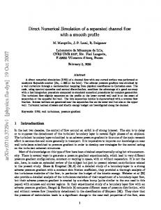
Figure 1: The time-averaged model of laminar separation bubble sketched by Horton [9].

13

Figure 2: The computational unstructured coarse mesh M1 for the flow past an Eppler 387 airfoil with 168,942 vertices.

14

-2.5 Mesh M1 Mesh M2 Mesh M3 Mesh Adaptive

-2

-1.5

Cp

-1

-0.5

0

0.5

1

1.5 -0.1

0

0.1

0.2

0.3

0.4

0.5

0.6

0.7

0.8

0.9

1

1.1

x/c

Figure 3: Mesh convergence of the pressure coefficient distribution over the Eppler 387 airfoil at α = 6◦ and Re=60,000.

0.08

1.08 1.06

0.07

1.04

0.06 1.02

0.05

Cd

Cl

1 0.98 0.96

0.04

0.03

0.94

0.02 0.92

0.01

0.9 0.88 0.7

0.702

0.704

0.706

0.708

0.71

0.712

0.714

0 0.7

0.716

0.702

0.704

0.706

0.708

0.71

0.712

0.714

0.716

t

t

Figure 4: Variation of lift and drag coefficients with time around an Eppler 387 airfoil at α = 6◦ and Re=60,000.

15

t=0

t = 1/4T

t = 2/4T

t = 3/4T

Figure 5: Several snapshots of vorticity magnitude contours around an Eppler 387 airfoil at α = 6◦ and Re=60,000.

16

-2.5

0.08

-2

0.06 t=0

-1.5

0.04

-1

0.02

Cf

Cp

t=0

-0.5

0

0

-0.02

0.5

-0.04

1

-0.06

1.5 -0.1

0

0.1

0.2

0.3

0.4

0.5

0.6

0.7

0.8

0.9

1

-0.08 -0.1

1.1

0

0.1

0.2

0.3

0.4

x/c

0.5

0.6

0.7

0.8

0.9

-2.5

0.06 t=1/4T

-1.5

0.04

-1

0.02

Cf

Cp

t=1/4T

-0.5

0

0

-0.02

0.5

-0.04

1

-0.06

0

0.1

0.2

0.3

0.4

0.5

0.6

0.7

0.8

0.9

1

-0.08 -0.1

1.1

0

0.1

0.2

0.3

0.4

x/c

0.5

0.6

0.7

0.8

0.9

-2

0.06 t=2/4T 0.04

-1

0.02

Cf

Cp

t=2/4T

-0.5

0

0

-0.02

0.5

-0.04

1

-0.06

0

0.1

0.2

0.3

0.4

0.5

0.6

0.7

0.8

0.9

1

-0.08 -0.1

1.1

0

0.1

0.2

0.3

0.4

x/c

0.5

0.6

0.7

0.8

0.9

1

1.1

x/c

-2.5

0.08

-2

0.06 t=3/4T

t=3/4T

-1.5

0.04

-1

0.02

Cf

Cp

1.1

0.08

-1.5

-0.5

0

0

-0.02

0.5

-0.04

1

-0.06

1.5 -0.1

1

x/c

-2.5

1.5 -0.1

1.1

0.08

-2

1.5 -0.1

1

x/c

0

0.1

0.2

0.3

0.4

0.5

0.6

0.7

0.8

0.9

1

-0.08 -0.1

1.1

x/c

0

0.1

0.2

0.3

0.4

0.5

0.6

0.7

0.8

0.9

1

1.1

x/c

Figure 6: Computed pressure (left) and skin friction (right) coefficients for an Eppler 387 airfoil at several different time levels t = 0, t = T /4, t = 2T /4 and t = 3T /4 at α = 6◦ and Re=60,000. 17

Figure 7: Computed mean vorticity contours (upper), pressure contours (middle) and streamtraces (bottom) around an Eppler 387 airfoil at α = 6◦ and Re=60,000.

18

-2.5 Present McGhee et al.

-2

-1.5

Cp

-1

-0.5

0

0.5

1

1.5 -0.1

0

0.1

0.2

0.3

0.4

0.5

0.6

0.7

0.8

0.9

1

1.1

0.6

0.7

0.8

0.9

1

1.1

x/c

0.08

0.06

0.04

Cf

0.02

0

-0.02

-0.04

-0.06

-0.08 -0.1

0

0.1

0.2

0.3

0.4

0.5

x/c

Figure 8: Computed mean pressure and skin friction coefficients around an Eppler 387 airfoil at α = 6◦ and Re=60,000.

19

0.92

0.88

Cl

0.84

0.8

0.76

0.72 0.66

0.67

0.68

0.69

0.7

0.71

0.72

0.73

0.74

0.75

0.76

0.77

0.78

0.79

0.8

0.81

0.82

0.75

0.76

0.77

0.78

0.79

0.8

0.81

0.82

t

0.1

0.09

Cd

0.08

0.07

0.06

0.05

0.04 0.66

0.67

0.68

0.69

0.7

0.71

0.72

0.73

0.74

t

Figure 9: Variation of three-dimensional lift and drag coefficients with time around an Eppler 387 airfoil at α = 6◦ and Re=60,000.

20

Figure 10: Computed vorticity magnitude iso-surfaces around an Eppler 387 airfoil at α = 6◦ and Re=60,000.

21

Figure 11: Computed vorticity magnitude contours at z/c = 0.25 plane for the flow past over an Eppler 387 airfoil at α = 6◦ and Re=60,000.

22

-2.5

-2.5

-2

-2 t=0.764

t=0.772

-1.5

-1.5

-1

Cp

Cp

-1

-0.5

-0.5

0

0

0.5

0.5

1

1

1.5 -0.1

0

0.1

0.2

0.3

0.4

0.5

0.6

0.7

0.8

0.9

1

1.5 -0.1

1.1

0

0.1

0.2

0.3

0.4

x/c

0.5

0.6

0.7

0.8

0.9

-2.5

-2 t=0.788

-1.5

-1.5

-1

-1

Cp

Cp

t=0.780

-0.5

-0.5

0

0

0.5

0.5

1

1

0

0.1

0.2

0.3

0.4

0.5

0.6

0.7

0.8

0.9

1

1.5 -0.1

1.1

0

0.1

0.2

0.3

0.4

x/c

0.5

0.6

0.7

0.8

0.9

-2 t=0.796

t=0.804

-1.5

-1.5

-1

-1

Cp

Cp

1.1

-2.5

-2

-0.5

-0.5

0

0

0.5

0.5

1

1

1.5 -0.1

1.5 -0.1

0

0.1

0.2

0.3

0.4

0.5

0.6

0.7

0.8

0.9

1

1.1

0

0.1

0.2

0.3

0.4

x/c

0.5

0.6

0.7

0.8

0.9

1

1.1

x/c

-2.5

-2.5

-2

-2 t=0.812

t=0.820

-1.5

-1.5

-1

-1

Cp

Cp

1

x/c

-2.5

-0.5

-0.5

0

0

0.5

0.5

1

1

1.5 -0.1

1.1

-2.5

-2

1.5 -0.1

1

x/c

0

0.1

0.2

0.3

0.4

0.5

0.6

0.7

0.8

0.9

1

1.1

x/c

1.5 -0.1

0

0.1

0.2

0.3

0.4

0.5

0.6

0.7

0.8

0.9

1

x/c

Figure 12: Computed pressure coefficients at z/c = 0.25 at several different time levels for the flow past over an Eppler 387 airfoil at α = 6◦ and Re=60,000.

23

1.1

-2.5 Present 2D Present 3D McGhee et al.

-2

-1.5

Cp

-1

-0.5

0

0.5

1

1.5 -0.1

0

0.1

0.2

0.3

0.4

0.5

0.6

0.7

0.8

0.9

1

1.1

x/c

0.08

0.06 Present 2D Present 3D 0.04

Cf

0.02

0

-0.02

-0.04

-0.06

-0.08 -0.1

0

0.1

0.2

0.3

0.4

0.5

0.6

0.7

0.8

0.9

1

1.1

x/c

Figure 13: Computed mean pressure and skin friction coefficients at z/c = 0.25 around an Eppler 387 airfoil at α = 6◦ and Re=60,000.

24

Figure 14: Computed mean vorticity contours around an Eppler 387 airfoil at α = 6◦ and Re=60,000.

25

0.004

0.0035

0.003

Power

0.0025

0.002

0.0015

0.001

0.0005

0

0

0.05

0.1

0.15

0.2

0.25

0.3

0.35

0.4

0.45

0.5

0

0.05

0.1

0.15

0.2

0.25

0.3

0.35

0.4

0.45

0.5

λ /c

0.04

0.035

0.03

Power

0.025

0.02

0.015

0.01

0.005

0

λ /c

Figure 15: Spectral analysis of the the kinetic energy along the spanwise line at point (0.75c, 0.1c) (upper) and point (1.0c, 0.1c) (lower) for an Eppler airfoil at α = 6◦ and Re=60,000.

26

0.004

0.0035

0.003

Power

0.0025

0.002

0.0015

0.001

0.0005

0

0

0.1

0.2

0.3

0.4

0.5

0.6

0.7

0.8

0.9

1

0

0.1

0.2

0.3

0.4

0.5

0.6

0.7

0.8

0.9

1

λ /c

0.04

0.035

0.03

Power

0.025

0.02

0.015

0.01

0.005

0

λ /c

Figure 16: Spectral analysis of the the kinetic energy along the spanwise line at point (0.75c, 0.1c) (upper) and point (1.0c, 0.1c) (lower) for an Eppler airfoil at α = 6◦ and Re=60,000 with 0.0 ≤ z/c ≤ 1.0.

27

-2.5

-2

Span=0.5c Span=1.0c McGhee et al.

-1.5

Cp

-1

-0.5

0

0.5

1

1.5 -0.1

0

0.1

0.2

0.3

0.4

0.5

0.6

0.7

0.8

0.9

1

1.1

x/c

Figure 17: The variation of pressure coefficients with spanwise length at z/c = 0.25 around an Eppler 387 airfoil at α = 6◦ and Re=60,000.

28