74
IEEE TRANSACTIONS ON RELIABILITY, VOL. 59, NO. 1, MARCH 2010
Direct Prediction Methods on Lifetime Distribution of Organic Light-Emitting Diodes From Accelerated Degradation Tests Jong In Park and Suk Joo Bae
Abstract—Accelerated degradation testing (ADT) expedites product degradation by stressing the product beyond its normal use. To extrapolate the product’s reliability at use condition, the ADT requires a known functional link relating the harsh testing environment to the usual use environment. Practitioners are often faced with a great challenge to designate an explicit form of the stress-degradation relationship a priori in accelerated degradation models. In this paper, we propose three methods to make direct inference on the lifetime distribution itself without invoking arbitrary assumptions on the degradation model: delta approximation, multiple imputation of failure-times, and the lifetime distribution-based (LDB) method. The methods are easy to implement without computational difficulty, hence they have potential in a wide range of applications for estimating lifetime distributions from ADT data. We applied the methods to two ADT data sets including a real application of commercial organic light-emitting diodes (OLED). The analysis of the examples and simulation results suggests parametric LDB and multiple imputation method as more potential alternatives to traditional failure-time approaches, especially for the case where there is neither enough physical background, nor historical evidence supporting presumed relationships between stress and the parameters of the degradation model.
LDB
lifetime distribution-based
LED
light-emitting diode
LRT
likelihood ratio test
OLED
organic light-emitting diode
ML
maximum likelihood
MVN
multivariate -normal
NRC
nonlinear random-coefficients
PDP
plasma display panel
SAFT
scale-accelerated failure-time NOTATION
Index Terms—Accelerated degradation test, delta approximation, lifetime distribution-based procedure, multiple imputation, nonlinear random-coefficients model, organic light-emitting diode.
ACRONYM1 ADT
accelerated degradation testing
ALT
accelerated life testing
LB
Lindstrom & Bates
LCD
liquid crystal display
,
Manuscript received January 11, 2009; revised July 06, 2009 and August 04, 2009; accepted August 13, 2009. First published February 17, 2010; current version published March 03, 2010. This work was supported by the Korea Research Foundation Grant funded by the Korean Government (MOEHRD, Basic Research Promotion Fund) (KRF-2007-331-D00539). Associate Editor: J.-C. Lu. The authors are with the Department of Industrial Engineering, Hanyang University, Seoul, Korea (e-mail:
[email protected];
[email protected]. kr). Color versions of one or more of the figures in this paper are available online at http://ieeexplore.ieee.org. Digital Object Identifier 10.1109/TR.2010.2040761 1The
singular and plural of an acronym are always spelled the same.
,
state matrix of stochastic variables time-scaled acceleration factor vector of random effects true degradation path predetermined threshold level activation energy (eV) probability density function of failure-times failure-times distribution baseline failure-times distribution variance function in accelerated degradation model likelihood function reaction rate in the Arrhenius relationship stress at usual use, and th stress level for , respectively heteroscedasticity parameter vector of fixed effects correlation parameter characteristic decay rates in bi-exponential model cumulative distribution function of a standard normal distribution mean lifetime at stress variance-covariance matrix of parameter vector of a degradation model for th individual at th stress level -normally distributed random error maximum likelihood estimate
0018-9529/$26.00 © 2010 IEEE Authorized licensed use limited to: Hanyang University. Downloaded on March 17,2010 at 21:26:08 EDT from IEEE Xplore. Restrictions apply.
PARK AND BAE: DIRECT PREDICTION METHODS ON LIFETIME DISTRIBUTION OF ORGANIC LED
75
I. INTRODUCTION
R
ELIABILITY testing typically generates product lifetime data; but for some tests, covariate information about the wear and tear on the product during the life test can provide additional insight into the product’s lifetime distribution. This usage measurement, termed degradation, can be the physical parameters of the product (e.g., corrosion thickness on a metal plate), or merely indicated through product performance (e.g., the luminosity of a Light Emitting Diode (LED)). As the statistical tool for predicting the lifetime distribution from degradation data, degradation analysis is especially useful for tests in which soft failures occur; that is, the lifetime of the test item is said to end after the measured performance decreases to a predetermined threshold value that designates a non-functioning state, or an incipient failure. For example, LED may be considered to fail only after the luminosity degrades below a fixed measured limit. Lu & Meeker [18], and Lu et al. [20] developed. A procedure to estimate a lifetime distribution based on degradation data assuming their own degradation models. See Nelson [23] for general discussions, and detailed information about degradation analysis. Degradation testing and analysis is tied with Accelerated Life Testing (ALT) because both methods have evolved in recent years to suit reliability tests for which product lifetimes are expected to last far beyond the allotted test time. ALT is meant to expedite product failure during test intervals by stressing the product beyond its usual use. Accelerated Degradation Testing (ADT) combines these two approaches by testing products in harsh environments, and measuring the evidence of product degradation during the ALT. Meeker & Escobar [22] provided a practical guide for ADT modeling along with standard ALT formulas. Bagdonaviˇcius & Nikulin [5, Ch. 3] developed theoretical models for accelerated degradation processes with catastrophic failures. ADT can provide the experimenter with more opportunities to draw quick inference on the lifetime distribution of highly reliable test items at use condition, provided there is a known functional link that relates the harsh testing environment to the usual use environment. Suzuki et al. [35], Lu et al. [19], and Park & Yum [26] showed that ADT can have an advantage over ALT, especially when few failures are expected due to a high reliability of test units. The approaches available in the literature are based mainly on the relationship between stresses and parameters of a degradation model, and assumptions on the distribution of the model parameters. Such a relationship may be chosen through statistical fits, or from a scientific point of view, but it is not always obvious to judge whether it is suitable. This research is motivated by accelerated degradation testing data from Organic LED (OLED). Lifetime estimation from the ADT of OLED is more challenging because the degradation model is of a complicated form in terms of model parameters, often leading to computational difficulty, and even the relationship between stresses and the model parameters are not clear. Against such a condition, we propose several alternative approaches for estimating the lifetime distribution at use condition from accelerated degradation data. All the approaches are intuitively appealing because they make direct inference on the
Fig. 1. Basic inner structure of an OLED.
lifetime distribution itself. They are also easy to implement, and do not require intensive computation. Hence, they have potential utility in a wide range of applications to inference problems for the lifetime distribution based on degradation data. The paper is organized as follows. Our motivating OLED example is illustrated in Section II, and an accelerated degradation model is given in Section III. In Section IV, three methods for estimating the lifetime distribution at use environment from the ADT model are illustrated. All the proposed methods are based on a Scale-Accelerated Failure-Time (SAFT) model to extrapolate the lifetimes in the use environment. In Section V, two practical applications of the ADT, Device-B and OLED examples, are analyzed following the proposed approaches. Some simulation results are given in Section VI, and discussions and concluding remarks are presented in Section VII. II. MOTIVATED EXAMPLE: ADT OF THE OLED OLED is a kind of LED whose emissive electroluminescent layer is comprised of a film of organic compounds. OLED is being vigorously developed as an alternative display because it possesses several advantages over other display devices such as Liquid Crystal Display (LCD), and LED: self-emission, large intrinsic viewing angle, and fast switching speed. The basic structure of a commonly used OLED is shown schematically in Fig. 1. In light display devices, luminosity is the most important performance characteristic, and a failure is defined by how much the luminosity decreases over time. The variable of interest is the amount of change from an initial luminosity level, while industry standards define a failure at the time when a device luminosity falls below 50% of its initial luminosity. There are a number of arguing causes of luminosity degradation. Among them, commonly recognized causes of luminosity degradation are [1], [34]: • formation of non-emissive dark spots; • long-term intrinsic decrease in the electroluminescence (EL) efficiency; and • morphological changes in the hole-transport layer, and/or degradation at the hole-injecting contact. Baldo & Forrest [6] illustrated the luminosity degradation of OLED in terms of density decreases of guest and host triplet excitons, and they modeled actual degradation paths with a bi-exponential model
Authorized licensed use limited to: Hanyang University. Downloaded on March 17,2010 at 21:26:08 EDT from IEEE Xplore. Restrictions apply.
(1)
76
IEEE TRANSACTIONS ON RELIABILITY, VOL. 59, NO. 1, MARCH 2010
where , and are constants determined by the initial conditions; and , and are characteristic decay rates of the guest, and the host triplet excitons, respectively. The bi-exponential model, often called the “two-compartment model,“ was also used to describe the degradation of OLED by Savvate’ev et al. [31], and Racine et al. [29]. Bae et al. [4] used the bi-exponential model to describe the mechanics of Plasma Display Panel (PDP) brightness degradation by incorporating nano-contamination effects during a series of manufacturing processes. However, because the bi-exponential model is not of the form that explicitly expresses the relationship between stresses and parameters of a degradation model in ADT, existing methods for deriving the failure-time distribution at the usual use environment from accelerated testing data can not be directly applied to the ADT data of the OLED. III. ACCELERATED DEGRADATION MODEL A. Nonlinear Random-Coefficients Model Suppose that the ADT of a product is conducted at higher , where is the stress at the stress levels: usual use environment. The observed sample degradation path at measurement time on the th individual test item under stress is given by level
(2) is the true degradation path at time under where may be a linear or nonlinear function of , stress level . and parameter vector , but we consider a nonlinear function of in this case. is assumed to be -independent of . Each product possibly experiences different sources of variation during fabrication. Hence, a degradation model with a random degradation rate is more appropriate for individuals to capture item-to-item variability of the degradation process. By introducing a random-coefficients model, we can easily incorporate individual variability into the degradation model. Allowing for flexible variance-covariance structures including heteroscedasticity or correlation structures within individual items, a random-coefficients model has been widely applied to repeated-measurement data arising in various applications such as economics, and pharmacokinetics. See Davidian & Giltinan [9] for a thorough overview on random-coefficients models. In particular, a nonlinear random-coefficients (NRC) model has many successful applications in handling complicated forms of degradation paths (e.g., Bae & Kvam [2], and Bae et al. [4]). Under a general formulation of the NRC model, the degradation model (2) can be represented as (3) , , and . Function denotes a variance function which expresses the heteroscedasticity with paramfor power eter (e.g.,
where
variance function), or correlation among within-individual measurements ruled by correlation parameter . Individual-specific is represented with a vector of fixed regression parameter effects , which is common for all individuals at stress , and a vector of random effects , which expresses between-indiis specific to th item at th vidual variation, i.e., depends on stress level. It is reasonable to assume that , but not on the item because the level of degradation is generally a function of the stress level only. At a particular stress , maximum likelihood (ML) estimation for the model parameters in (3) is based on the marginal density of (4) is the conditional density of given where the random effects having the marginal distribution . can Note that (4) is only valid for the soft failures where still be observed even after the true degradation has crossed the threshold value. In general, because this integral does not have a closed-form expression when the model function is nonlinear in , approximation methods, such as Lindstrom & Bates’ (LB) algorithm [17], and adaptive Gaussian quadrature [27], can be used to estimate the marginal density (4). Bae & Kvam [2] introduced various approximation methods to numerically optimize the log-likelihood corresponding to (4), and evaluated them in terms of some comparison criteria for non-monotonic degradation paths of vacuum fluorescent displays at a stress level. B. Deriving Lifetime Distribution To derive the failure-time distribution and its quantiles from accelerated degradation data, define failure-time as the first crossing time that the actual degradation path reaches . Using the form of for simplicity, the distribution of the failure-time is
(5) At a specific level of the accelerating variable, the failure-time distribution depends on the distribution of the random coefficient , which is determined by . Denote the true value of as . Within the framework of (3), the failure probability at a given time can be expressed as
(6) , and can be computed by reML estimates of the with ML estimates of the parameters . placing Evaluation of (6) usually relies on Monte Carlo simulation due to the complexity of analytical approaches [22]. When the lifetime distribution at usual use environment is estimated by using (6) based upon the accelerated degradation data, incorporation of the effects of stress variables requires additional assumptions for a functional relationship between stress in the degradation model. Such variables and the parameters a relationship may arise from substantive knowledge in the area
Authorized licensed use limited to: Hanyang University. Downloaded on March 17,2010 at 21:26:08 EDT from IEEE Xplore. Restrictions apply.
PARK AND BAE: DIRECT PREDICTION METHODS ON LIFETIME DISTRIBUTION OF ORGANIC LED
of application, or may be suggested by examining the data [40]. However, it poses a great challenge on practitioners to make a reasonable assumption for the relationship. Furthermore, as Tseng & Peng [36] pointed out, existing approximation methods do not always guarantee precise estimation for , even when a well-known relationship is given. In the following section, we propose three alternative methods for estimating the lifetime distribution under the use environment based on accelerated degradation data. All the methods assume a SAFT model [22, Ch. 17] to extrapolate lifetime distributions at a predefined use environment from the accelerated conditions. IV. LIFETIME ESTIMATION BASED ON ADT DATA Under the SAFT model, the failure-time of a unit at a certain stress level can be obtained by simply multiplying its failuretime at any other stress level by the acceleration factor. With , that is the distribution funcbaseline distribution function tion at use stress level , the distribution function at stress is given by (7) is a time-scaled acceleration factor at . For where than , in the sense that time higher stress than at . moves more quickly at The SAFT model is relatively simple to interpret, but we should be selective in our use of the SAFT model because it does not hold universally. Luvalle et al. [21] described more general degradation model characteristics needed to assure that the SAFT property holds. The SAFT model is often suggested by the physical theory for some simple failure mechanisms; for example, in the Arrhenius relationship describing the effects of temperature on the rate of a simple chemical reaction, the acceleration factor is
77
A. Delta Approximation of Lifetime Distribution given is norBecause the conditional probability of mally distributed, the failure probability in (6) can be re-written as
(11) For non-monotonic (e.g., an example of vacuum fluorescent displays in [2]), (11) may not be correct. In this paper, we only consider monotonic and nonlinear degradation paths . Hence, . In general, the assumption is valid because most degradation paths degrade monotonically, such as in our examples presented is nonlinear in , there may be no later. If the function of closed-form expression for the expectation in (11). We propose delta approximation [15, Ch. 2.5] to derive the expectation by expanding the Taylor series with respect to . For all in the , it is assumed that is neighborhood of monotone with respect to . It is difficult to exhibit tractable conditions on and for this condition to hold in the general framework of a nonlinear random-coefficients model. However, it is relatively simple to show the monotonicity of in our practical examples by checking that the set of for is increasing with respect which is decreasing to is the same as the set of for which with respect to . By considering a second-order Taylor series expansion about of (i.e., delta approximation), we can approximate (11) as
(8) , and represent the reaction rates at , and where , respectively. is the activation energy in electron volts is Boltzmann’s constant in electron (eV), volts per , and is temperature in the absolute Kelvin scale. As another model describing the effects of temperature on the reaction rate, the Eyring relationship temperature-acceleration factor [13] is (12) (9) where is a constant ranging between 0 and 1 [23]. In the inverse power relationship, which is the most commonly used model for voltage acceleration, the acceleration factor is expressed as (10)
for -dimensional random-coefficients . Note that the second . term in the right-hand side is 0 because Given ML estimates of , we can easily calculate the failure probability at each stress level using (12). Time-scaled transformations such as (7) are then used to obtain the lifetime distribution at use environment. Define a scale factor between , and ; for . Then can be estimated as
is the material-specific exponent. See Meeker & where Escobar [22] for more details. Authorized licensed use limited to: Hanyang University. Downloaded on March 17,2010 at 21:26:08 EDT from IEEE Xplore. Restrictions apply.
(13)
78
IEEE TRANSACTIONS ON RELIABILITY, VOL. 59, NO. 1, MARCH 2010
where is an estimated mean lifetime at stress obtained as
, and it can be
with respect to and , , the number of different estimators of is . These estimators are combined to obtain a pooled estimator of [33]:
In this study, we apply Dorey et al.’s procedure [11] among the existing multiple-imputation techniques. They presented various approaches multiplying imput values for the threshold-crossing times of some prognostic variables in medical studies. The crossing times are often unknown because patients’ conditions may be periodically examined, but not continuously. They modeled the values at some time between data-collection points via simple linear regression models to execute multiple imputations. Instead of simple linear regression models, the degradation model in (3) is taken into account here. The steps to derive an approximate lifetime distribution, based on the imputation procedure, are as follows. Step 1) For each stress , estimate pseudo lifetimes, and relating errors: , the pseudo lifeGiven the MLE time of the th test unit can be calculated as , and the measurement error at is estimated by
(16)
(19)
at use stress level is then
for -dimensional fixed effects . Here, is total number of measurements for all test items at stress . Approximate standard error for the pseudo lifetimes is
(14) is the cumulative distribution function evaluated at . Because the integration in (14) is not tractable in practice, numerical integration methods can be applied instead. , To estimate the lifetime distribution at use stress level with we need to incorporate some acceleration models here. For example, in the inverse power relationship under the SAFT model is defined as (7), where
(15) For an estimator of
The cumulative distribution computed by
(17) where
for
(20)
.
B. Multiple Imputation of Failure-Times Even with little or no failures during the test period, failuretimes of each item can be obtained by extrapolating the times when their degradation paths would first cross the pre-specified . Associated with the general degradation path model level in Section III, those failure-times can be expressed via pseudo failure-times (18) for estimating the lifetime distribution of degradation data. However, such a method has drawbacks. One major drawback is that it neglects any sort of errors such as the prediction error, and measurement error in extrapolating failure-times [22]. Meanwhile, the so-called multiple imputation method has been widely applied as a technique for handling data sets with missing values since first proposed by Rubin [30]. It replaces each missing value with several completed data sets created by a fully randomized procedure. Each data set is separately analyzed using standard complete-data methods, then the results are combined to give a final result. In recent years, much attention has been placed particularly on extending the idea to generate exact failure-times from censored data (e.g., right-censored, and interval-censored data) for estimating survival functions [7], [25], [39]. The pseudo failure-times in (18) are augmented data in that they fill in the unknown exact failure-times. The potential bias of the conventional method is expected to be minimized by exploiting the imputation procedures that incorporate error terms in a reasonable fashion when generating the pseudo data.
where
Here, mensions of respectively,
.. .
,
, and , and
,
.. .
.. .
..
.
; and the diare, .
.. .
where is the actual degradation path in (3) for the th test item at stress . , draw Step 2) For each th set of imputation as a random value of (21) is a chi-square random variable with dewhere . grees of freedom Step 3) Given the drawn value of , the imputed value for the th set is (22) where is a random variate generated from a standard normal distribution.
Authorized licensed use limited to: Hanyang University. Downloaded on March 17,2010 at 21:26:08 EDT from IEEE Xplore. Restrictions apply.
PARK AND BAE: DIRECT PREDICTION METHODS ON LIFETIME DISTRIBUTION OF ORGANIC LED
Step 4) Check if the imputed value lies in the failure interval . The interval is constructed by actual failure observed interval for for (23) where , and denote the sets of test units whose failure times are observed, and censored, respecis the termination time for degratively; and dation measurements of the th unit. If , then go to Step 3. Otherwise, repeat Step 2 through Step 4 until complete data sets are created. Shaked et al.’s approach [33] presented in the previous secfor each tion can be exploited again to estimate , and data set of imputation; that is, the estimates are
for
, and number of
In the inverse power relationship, for example, for , and . Then are combined to give a final estimate of at the use condition [11]: (24)
79
fails. The failure-times, called interval-censored failures, may be combined with degradation observations to make inference on product lifetimes, as in the work of Padgett & Tomlinson [24]. However, the LDB procedure does not assume any failure implicitly when adjusting predictive intervals of individual lifetimes to degradation measurement points. This assumption may lead to predictive intervals failing to cover actual failures. We propose a modified version of the LDB procedure to remedy such a biased outcome. Another limitation to the application of the LDB procedure is that the lifetime distribution should be specified by users in advance. Some authors recommended strategies for choosing the most proper distribution among the candidates. In particular, Bae et al. [3] asserted that careful attention should be paid before assuming the lifetime distribution for degradation data because the assumption of the degradation model may create a strong restriction on the lifetime distribution. To minimize the risk of model mis-specification, we introduce an empirical method rather than assuming a specified lifetime distribution: a logspline density estimation. The logspline density estimation is easier to implement than the popular kernel density estimation in which determination of the optimal bandwidth often requires laborious tasks [14]. From the degradation analysis, predictive interval estimates with a confidence for lifetimes at each stress level can be calculated by and (25) is the th quantile of the standard normal diswhere tribution. Using the failure information given as in (23), these estimates are converted into a new interval as
C. Lifetime Distribution Based (LDB) Procedure A Lifetime Distribution Based (LDB) procedure, which was first proposed by Chen & Zheng [8], is to choose a set of parameters that gives the largest likelihood for a given lifetime distribution. The procedure exploits estimates of individual lifetimes from the degradation analysis. The procedure consists of two steps: degradation modeling, and imputation steps. First, predictive intervals of individual lifetimes are constructed by modeling the degradation paths. Then a recursive algorithm is implemented to obtain estimates of the lifetime distribution such that the likelihood function is maximized. The LDB procedure can be easily implemented because it assumes a one-dimensional lifetime distribution, while conventional methods (e.g., Lu & Meeker’s two-stage method [18]) may require manipulation of multi-dimensional parameters in the degradation model. Chen & Zheng [8] reported that the LDB procedure provides better performance than the existing methods, especially when many failures are observed during a given testing period. In this study, we suggest some modifications for the LDB procedure to effectively apply to accelerated degradation data. Along with observed levels of degradation, some information on failures can be obtained during the accelerated degradation testing. In practice, because the degradation amount of a testing item is intermittently measured at certain points in time, we can only observe specific time intervals over which the item
for for elsewhere
(26)
The estimate of the lifetime distribution is produced from the following algorithm. Step 1) Obtain the individual lifetimes by calculating the conditional expectation
(27)
where , and are a probability density function, and a distribution function of the lifetimes, reis the th estimate of the paspectively. Here, rameter vector of a lifetime distribution at stress . Step 2) Find a new estimate of maximizing the log-likelihood as (28) Repeat Step 1 through Step 2 until convergence occurs.
Authorized licensed use limited to: Hanyang University. Downloaded on March 17,2010 at 21:26:08 EDT from IEEE Xplore. Restrictions apply.
80
IEEE TRANSACTIONS ON RELIABILITY, VOL. 59, NO. 1, MARCH 2010
Fig. 2. Accelerated degradation testing data of power drop in Device-B over time at three temperature levels [22].
For the density , either known functions (e.g., Weibull, and lognormal) or the logspline density function can be taken as (29) where
Here,
is the B-spline basis [10], and is the number of "knots". In the logspline density estimation, the smooth function is fitted to the log-density function of the lifetimes within subsets of the time axis defined by the knots, and constrained to be continuous at those points (see Kooperberg & Stone [14] for more details). For the case where lifetime distributions are specified, specific relationships between the distribution parameters and stress variables are employed to estimate the lifetime distribution at use environment. Nominal life at (transformed) stress level is expressed as (30) where is a transformed stress at the th level. In the Arrhenius , , and relationship for example, in the inverse power relationship. The nominal life is either a scale parameter for the Weibull distribution, or a location parameter for the lognormal distribution. The parameters , and are estimated by maximizing the log-likelihood
with respect to , and . denotes the final lifetime data derived from the above two-step algorithm. It may be impossible to assume the parametric linkage like (30) when employing the logspline density estimation. The nonparametric approaches can be applied to estimate for that situation.
Fig. 3. Predicted failure-time distributions at 195
C: Device-B example.
V. PRACTICAL APPLICATIONS A. Device-B Example In this part, we will illustrate application of the approaches proposed in the preceding section to ADT data of integrated circuit (IC) devices called "Device-B" in Meeker & Escobar [22]. Samples of the device were tested at each of three accelerated , 195 , and 237 . levels of junction temperature: 150 Failure of the device is defined as power output greater than 0.5 decibels (dB) below initial output. Fig. 2 shows the accelerated degradation testing data of power outputs over time at each temperature level. The purpose of this experiment is to estimate the junction temperlifetime distribution at use environment (80 ature). Meeker & Escobar [22] suggested the following simple degradation model with a temperature-acceleration factor:
Authorized licensed use limited to: Hanyang University. Downloaded on March 17,2010 at 21:26:08 EDT from IEEE Xplore. Restrictions apply.
(31)
PARK AND BAE: DIRECT PREDICTION METHODS ON LIFETIME DISTRIBUTION OF ORGANIC LED
TABLE I PREDICTED FAILURE-TIME DISTRIBUTION AND ITS QUANTILES AT NORMAL USE CONDITION (80
where is the rate reaction at the th temperature level for the Arrhenius acceleration factor given in (8), and is the asymptote. Following their approach, define , , and , where is the reaction rate at 195 . Such reaction term was employed to keep small the correlation and the parameters relating . between the estimates of The term representing the rate reaction and the asymptote are assumed to be random, describing item-to-item variability. , they For obtained ML estimates of the parameters using the nonlinear mixed-effects computer program by Pinheiro & Bates [27] as
and . In general linear models, the estimate of the failure-time discan be obtained by substituting the ML estimates tribution into (5). However, when there is no closed-form expression ; and when the numerical transformation methods are for overly complicated, Lu & Meeker [18] proposed the evaluausing Monte Carlo simulation. For this evaluation, tion of (realized by ) are the model parameter estimates , and used to generate the simulated realizations , and at the th stress level. From values of , and , compute the failure times by substituting , and into ; . For any desired values of , is estiand then solve for mated from the simulated empirical distribution number of (32) for . At each temperature level, the failure-time distributions for Device-B were derived following the proposed methods in the preceding section. For the parametric LDB procedure, Weibull, and lognormal distribution were taken as the assumed lifetime distribution because those are the most popular ones among existing lifetime distributions. We compared the results with the distribution estimate from Monte Carlo evaluation. For instance,
81
C): DEVICE-B EXAMPLE
at 195 showed that the lifetime distribution the plot of estimated by the Monte Carlo evaluation exhibits a much longer upper tail than other methods (see Fig. 3). Such a trend was also observed in Chen & Zheng [8]. Meanwhile, the Monte Carlo methods are computationally intensive, and require much time to estimate lifetime distributions from a large number of simulated degradation paths. However, our proposed methods are computationally efficient because they make direct inference on the lifetime distribution itself through degradation data. quantiles for the failure-time disThe point estimates and tribution at use environment (80 ) are summarized in Table I, for , 0.10, 0.50, and 0.90. All of the three proposed methods give different point estimates for the quantiles. Especially, the lifetime distribution estimated from the delta approximation is quite different from the others. Among the proposed methods, the parametric LDB-lognormal, and multiple imputation produce outcomes closer to those of the Monte Carlo method. B. OLED Example 1) Accelerated Degradation Testing of OLED: The degradation test for OLED was executed to assess the reliability of OLED at use environment. The test units in this application are samples of OLED devices used as display elements for mobile phones. Because the original data from this experiment are proprietary, we have disguised the original data by adding or subtracting values with the goal of not significantly affecting the overall analytical results. The degradation of OLED is mainly indicated by a decrease in its luminosity over time. Degradation mechanisms of the luminosity were accelerated using DC current. The testing data consist of measurements of luminosity for each unit at 20 time points. Ten test units are subjected at each of four accelerated stress levels: 25 mA, 32 mA, 40 mA, and 50 mA. The degradation paths at each DC current are given in Fig. 4. The purpose of this test is to estimate the lifetime distribution at use condition (6.4 mA). 2) OLED Degradation Analysis: We seek a model for relative luminosity by dividing each of the luminosity measurements by initial luminosity to easily derive the failure-time of the OLED, where the failure is defined at the time when the relbelow 50%. As ative luminosity falls below 0.5 or
Authorized licensed use limited to: Hanyang University. Downloaded on March 17,2010 at 21:26:08 EDT from IEEE Xplore. Restrictions apply.
82
IEEE TRANSACTIONS ON RELIABILITY, VOL. 59, NO. 1, MARCH 2010
Fig. 4. Accelerated degradation testing data of the OLED.
TABLE II ESTIMATED COEFFICIENTS (FIXED-EFFECTS) IN THE BI-EXPONENTIAL DEGRADATION MODEL AT EACH STRESS LEVEL: OLED EXAMPLE
shown in Fig. 4, all the luminosity of the OLED tend to decrease rapidly at the initial stage of degradation testing, then its degradation becomes more gradual. To capture the characteristics of OLED degradation, we introduce the bi-exponential model (1) to relative luminosity data. The testing data also suggest that the OLED degradation model should include variability among and within individual units, which can be efficiently modeled by introducing random-coefficients. Furthermore, because the measurements collected sequentially over time are basically timeseries data, we may need to include correlation in the error terms. The general degradation model for relative luminosity at each stress can be expressed as
(33) and . Because the rate constants for must be positive to be physically meaningful, we re-parameterized (1) in terms of the exponential-rate constants. Here, designates an autoregressive process with order as , where is a white noise with zero mean, and constant variance. The likelihood ratio test (LRT) was employed to compare NRC models fitted by maximum likelihood to decide which of the coefficients in the model requires random effects to account as the likelihood of a genfor between-unit variation. Denote
as the likelihood of a eral model with random effects, and restricted model with no random effects; then under the null hy, the likelihood ratio test statistic pothesis
will follow asymptotically a mixture of two distributions distribution. As described by Self & rather than a single Liang [32], the hypothesis test applies to nonstandard testing is the boundary point of the parameter situations because space, so the likelihood ratio test does not have a limiting distribution. Indeed, the optimal properties of the MLE, and likelihood ratio test are developed for the case when the true parameter is an inner point to be able to apply the Taylor series expansion. For example, in hypothesis tests of no random effects versus one random effect, the LRT statistic is a mixture and with equal weights of 0.5 each, where is the of distribution which gives probability mass one to the value 0. random In hypothesis tests of random effects versus and , again effects, the LRT statistic is a mixture of with equal weights. The model-building strategy is to start with the model with random coefficients for all parameters, and then examine the fitted model to decide which, if any, of the random coefficients can be eliminated from the model. By sequentially executing the LRT procedure, we choose the model with four random-coefficients having a general positive-definite covariance structure, and AR(1) structure for errors as the best model. All fixed-effect estimates of the model are summarized in Table II. For example, the fitted model for the data at 50 mA is
where
Authorized licensed use limited to: Hanyang University. Downloaded on March 17,2010 at 21:26:08 EDT from IEEE Xplore. Restrictions apply.
PARK AND BAE: DIRECT PREDICTION METHODS ON LIFETIME DISTRIBUTION OF ORGANIC LED
83
Fig. 5. The bi-exponential degradation model fit at 50 mA (bold line fits the random-coefficients model, and dot line fits fixed effects model ignoring unit-to-unit variation).
Fig. 6. Estimated mean curve plot of degradation at each stress level based on the bi-exponential model with random-coefficients.
and , where . Fig. 5 shows that the bi-exponential model fit with random-coefficients provides more reliable results in predicting true values of the OLED luminosity by well capturing both the nonlinearity of the degradation path, and the variability among test units, than the model ignoring between-individual variation (that is, a fixed effects model). From the bi-exponential model with random-coefficients, estimated mean curves of degradation at each stress level are displayed in Fig. 6.
3) OLED Failure-Time Analysis: Because the estimated coefficients in Table II have different stress-dependencies, it is not apparent how to express the stress-degradation relationship in the bi-exponential degradation model. Further, as pointed out by Pinheiro & Bates [28], the two sets of parameters in the first and second exponential terms are exchangeable without changing the values of predictions. This motivates application of the methods proposed in this study so that arbitrary incorporation of stress effects into the model can be avoided.
Authorized licensed use limited to: Hanyang University. Downloaded on March 17,2010 at 21:26:08 EDT from IEEE Xplore. Restrictions apply.
84
IEEE TRANSACTIONS ON RELIABILITY, VOL. 59, NO. 1, MARCH 2010
Fig. 7. Estimated lifetime distributions for OLED ADT data.
The failure-time distributions estimated by applying the proposed methods are plotted in Fig. 7. Partial derivatives needed to calculate (12) in the delta approximation, and (20)
in the multiple imputation, are provided in the Appendix. The curves at each stress level have similar shapes, but different scales. However, the curves by the delta approximation show
Authorized licensed use limited to: Hanyang University. Downloaded on March 17,2010 at 21:26:08 EDT from IEEE Xplore. Restrictions apply.
PARK AND BAE: DIRECT PREDICTION METHODS ON LIFETIME DISTRIBUTION OF ORGANIC LED
85
TABLE III PREDICTIVE INTERVALS OF INDIVIDUAL LIFETIMES FROM THE LDB PROCEDURE
slightly different patterns compared to the other methods. For the parametric LDB procedure, we used Weibull, and lognormal distributions as the assumed lifetime distribution. In the experiment, because many failures are observed, and the failure times are interval-censored, we can verify the validity of the predictive intervals for individual lifetimes calculated from the LDB procedure by checking if the intervals intersect with corresponding actual failure-intervals. Table III shows that many intervals from Chen & Zheng’s method [8] (highlighted with underlines) fail to embrace the actual (soft) failures, but our modified LDB methods successfully embrace all the failures, avoiding such biased outcomes. When a specific functional form for the lifetime distribution is assumed as in the parametric LDB procedure, we can check whether the SAFT model is applicable via statistical tests for equality of a distribution parameter (e.g., a shape parameter for Weibull distribution, and a scale parameter for lognormal dis-
tribution). In hypothesis tests for the equality of the distribution parameters, the Wald statistic [23] produced -values of larger than 0.10 for both the Weibull distribution (0.569), and the lognormal distribution (0.693), strongly supporting the validity of the SAFT model. In Fig. 8, distribution functions estimated from each method are re-exhibited at each stress level for comparison. Turnbull’s nonparametric estimates [37] calculated from the interval-censored failure data are also added in the plots to aid the comparison. While both multiple imputation and LDB procedure provide similar results on the lifetime distribution, the delta approximation tends to underestimate the true lifetime distribution, especially at higher stress levels. The multiple imputation is shown to give nearly the same estimates as Turnbull’s. The heavier the censoring, it is likely that the more the estimates from the three proposed methods deviate from Turnbull’s. Note that the Turnbull curve for 25 mA takes very few steps with high degree of
Authorized licensed use limited to: Hanyang University. Downloaded on March 17,2010 at 21:26:08 EDT from IEEE Xplore. Restrictions apply.
86
IEEE TRANSACTIONS ON RELIABILITY, VOL. 59, NO. 1, MARCH 2010
Fig. 8. Comparisons of lifetime distributions estimated by the proposed methods at each stress level.
TABLE IV CALCULATED ABSOLUTE BIASES AT EACH STRESS LEVEL
censoring in the small data set, thus the proposed methods no longer track the Turnbull’s curve closely. This feature is one of the advantages of using the degradation data, that the proposed methods can make inferences beyond the given data. Besides, they produce smoother, more interpretable estimates than the empirical estimates such as Turnbull’s, as shown in the figures. The comparison of general performance among the proposed methods was done in each stress level by calculating the absolute bias of the estimate of the cdf corresponding to each
method with respect to the Turnbull’s empirical cdf. Note that, unlike the estimates in Figs. 7 and 8, all of the estimates for bias calculations were obtained based on the remainder of the ADT data after deleting the data associated with the target stress conditions at which lifetimes are estimated, enabling us to compare the methods in terms of the generalization performance. As shown in Table IV, parametric LDB-lognormal, and multiple imputation give relatively small biases in comparison to other methods.
Authorized licensed use limited to: Hanyang University. Downloaded on March 17,2010 at 21:26:08 EDT from IEEE Xplore. Restrictions apply.
PARK AND BAE: DIRECT PREDICTION METHODS ON LIFETIME DISTRIBUTION OF ORGANIC LED
87
TABLE V COMPARISON OF MEAN LIFETIME ESTIMATES AT THE USE CONDITION, AND ACCELERATION COEFFICIENT ESTIMATES
Assuming an inverse power relationship for DC current acceleration, we estimated the acceleration coefficient in (15) by applying the three methods to the accelerated testing data, then extrapolated the mean lifetime at the use environment (6.4 mA). Bootstrap confidence intervals were also obtained to check how stable the methods give parameter estimates. In this case, bootstrap samples were generated at each of the four stress levels. Comprehensive review of the theory and practice of the bootstrap method are given in Efron & Tibshirani [12]. The estimation results are summarized in Table V, along with 95% bootstrap confidence intervals (in parentheses). The lifetime estimates from the delta approximation are the shortest, while the LDB-logspline and multiple imputation provide estimates roughly between LDB-Weibull’s and LDB-lognormal’s. Also observe that the confidence intervals for mean lifetimes are largest when applying the delta approximation. VI. SIMULATION RESULTS We use simulated ADT data to suggest guidelines as to which of the three methods can be preferred in various situations. We generated ADT data from the simpler degradation model (31) rather than a computationally intensive bi-exponential model for comparison convenience. Ten degradation paths were gen), erated at each of three temperature levels (150, 195, 237 using the same inspection schemes (e.g., inspection intervals, and termination time). We used the same values of ML estimates , and (which were obtained by fitting the degradation paths to the NRC model (31) in the Device-B example) for simulation. Instead, we varied the within-individual varito examine the change ance as of lifetime estimation at the usual use environment according to within-individual variation. Based on simulated ADT data, at use environment (80 we estimated the th quantiles ), using the proposed methods for , and 0.9. We repeated the simulation 100 times. The resulting aver, are ages of relative mean square errors (MSE), summarized in Table VI, along with corresponding absolute relin parentheses. True quantile values ative biases were calculated through Monte Carlo evaluation with the assumed estimates of the NRC model. As shown in Table VI, the LDB-lognormal method gives the smallest MSE and bias for almost all the quantiles. On the other
hand, it turns out that the quantile estimates obtained from the delta approximation are quite dissimilar to those from the other methods, with the values almost unchanged for all values. The delta approximation gives relatively poor results, while its values of MSE and bias for the 0.5 quantile are better than those of the other methods. We observed, through another simulation, that the delta approximation often shows this odd behavior, especially when between-individual variation is much larger than , because the second and third within-individual variance term in (12) can not be stably evaluated in this situation. Noticeably, the MSE obtained from the delta approximation tends to increase as within-individual variance decreases, while the MSE from the other methods tend to decrease expectedly. In conclusion, the delta approximation may fail to produce reliable estimates for lifetime distributions at usual use conditions. To summarize the two real examples, and the simulation results, parametric LDB methods are more likely to provide relatively unbiased stable estimates than the other methods. However, when the proper lifetime distribution is unknown, both multiple imputation, and nonparametric LDB methods may be a good alternative in that their performance are not remarkably poor compared to the parametric LDB methods. Especially, the former can be used for estimating lower quantiles, and the latter for upper quantiles. VII. DISCUSSIONS, AND FUTURE RESEARCHES We have examined how reliability prediction can be simply implemented in the new frameworks for accelerated degradation data. The proposed methods make direct inference on the lifetime distribution using either simple approximation, or imputed lifetime data. The approaches also enable practitioners to avoid making subjective assumptions by directly incorporating the effects of physical stresses into the degradation model. By applying the methods to real-life examples, we compared their performance with the conventional approaches including the Monte Carlo evaluation, and Turnbull’s method. It can be observed that the lifetime distributions estimated by the proposed methods are close to the empirical distribution based on the actual failure data. This result suggests that the methods be potential alternatives to traditional failure-time methods, especially for the case where there is neither enough physical background, nor historical evidence supporting presumed relationships between stress variables, and the parameters in the degradation model.
Authorized licensed use limited to: Hanyang University. Downloaded on March 17,2010 at 21:26:08 EDT from IEEE Xplore. Restrictions apply.
88
IEEE TRANSACTIONS ON RELIABILITY, VOL. 59, NO. 1, MARCH 2010
TABLE VI COMPARISON AVERAGE OF RELATIVE MEAN SQUARE ERRORS (MSE) FOR pth QUANTILE ESTIMATES AT USE ENVIRONMENT (80 CORRESPONDING ABSOLUTE RELATIVE BIASES IN PARENTHESES
The proposed methods, however, have further investigations required for extensive applications: • In some products, multiple failure-causing chemical reactions may exist, probably causing the SAFT assumption across applied stress levels to not be suitable. A natural generalization of the SAFT model is to impose stress-de-
C), ALONG WITH
pendence upon both shape, and scale (or scale, and location in a lognormal distribution) parameters of the lifetime distribution. There have been a few reports on the models and data analysis methods for problems with non-constant shape (or scale) parameter of the lifetime distributions. For an example, Wang & Kececioglu [38] proposed an effi-
Authorized licensed use limited to: Hanyang University. Downloaded on March 17,2010 at 21:26:08 EDT from IEEE Xplore. Restrictions apply.
PARK AND BAE: DIRECT PREDICTION METHODS ON LIFETIME DISTRIBUTION OF ORGANIC LED
cient algorithm to obtain the MLE of the Weibull log-linear model with the stress-dependent shape parameter. It would be useful to extend this study to encompass such a generalization. • Competing risk problems involving both soft failures, and catastrophic failures are often found in various real applications. It would be possible to include catastrophic failure data under the current configuration by making inference on the lifetime distributions assuming the competing risks. • This article assumes deterministic operating conditions at use environment. However, products in field applications are often subjected to dynamic environments. For instance, the mobile phones with OLED displays may have different display modes according to operating environments (e.g., time, and location of use), or service conditions (e.g., phone call, or wireless internet connection). Each mode requires different amounts of current flow, so operating stress varies stochastically. Liao & Elsayed [16] warned that ignoring such stress variations would lead to significant flaws in correctly evaluating field reliability. The further study can include the extension to stochastic operation stresses for the ADT data.
89
Partial Derivatives in (20) Under the Model (33) for
Let then
,
where , and standard normal distribution. Under the model (33),
denotes the pdf of a
for for
APPENDIX for
, and 0 for
.
Partial Derivatives in (12) Under the Model (33) For notational convenience, subscripts that stand for stress levels and samples are omitted.
for and 0, for
for for For , which is the value of satisfying with the equation
ACKNOWLEDGMENT The authors would like to thank the anonymous referees who helped gain substantial improvements in the manuscript. The authors are very grateful to Mr. Y. H. Huh for providing the OLED data. REFERENCES
where
for
. Here,
[1] H. Aziz, Z. D. Popovic, N.-X. Hu, A.-M. Hor, and G. Xu, “Degradation mechanism of small molecule-based organic light-emitting devices,” Science, vol. 283, pp. 1900–1902, 1999. [2] S. J. Bae and P. H. Kvam, “A nonlinear random-coefficients model for degradation testing,” Technometrics, vol. 46, pp. 460–469, 2004. [3] S. J. Bae, W. Kuo, and P. H. Kvam, “Degradation models and implied lifetime distributions,” Reliability Engineering & System Safety, vol. 92, pp. 601–608, 2007. [4] S. J. Bae, S.-J. Kim, M. S. Kim, B. J. Lee, and C. W. Kang, “Degradation analysis of nano-contamination in plasma display panels,” IEEE Trans. Reliability, vol. 57, pp. 222–229, 2008. [5] V. Bagdonavièius and M. Nikulin, Accelerated Life Models: Modeling and Statistical Analysis. New York: Chapman & Hall, 2001. [6] M. A. Baldo and S. R. Forrest, “Transient analysis of organic electrophosphorescence: I. Transient analysis of triplet energy transfer,” Physical Review B, vol. 62, pp. 10 958–10 966, 2000.
Authorized licensed use limited to: Hanyang University. Downloaded on March 17,2010 at 21:26:08 EDT from IEEE Xplore. Restrictions apply.
90
IEEE TRANSACTIONS ON RELIABILITY, VOL. 59, NO. 1, MARCH 2010
[7] J. D. Bebchuk and R. A. Betebsky, “Multiple imputation for simple estimation of the hazard function based on interval censored data,” Statistics in Medicine, vol. 19, pp. 405–419, 2000. [8] Z. Chen and S. Zheng, “Lifetime distribution based degradation analysis,” IEEE Trans. Reliability, vol. 54, pp. 3–10, 2005. [9] M. Davidian and D. M. Giltinan, Nonlinear Models for Repeated Measurement Data. London: Chapman & Hall, 1995. [10] C. de Boor, A Practical Guide to Splines. New York: Springer-verlag, 2001, revised edition. [11] F. J. Dorey, R. J. A. Little, and N. Schenker, “Multiple imputation for threshold-crossing data with interval censoring,” Statistics in Medicine, vol. 12, pp. 1589–1603, 1993. [12] B. Efron and R. J. Tibshirani, An Introduction to the Bootstrap. New York: Chapman & Hall, 1993. [13] H. Eyring, Basic Chemical Kinetics. New York: Wiley, 1980. [14] C. Kooperberg and C. J. Stone, “A study of logspline density estimation,” Computational Statistics & Data Analysis, vol. 12, pp. 327–347, 1991. [15] E. L. Lehmann, Elements of Large-Sample Theory. New York: Wiley, 1998. [16] H. Liao and E. A. Elsayed, “Reliability inference for field conditions from accelerated degradation testing,” Naval Research Logistics, vol. 53, pp. 576–587, 2006. [17] M. J. Lindstrom and D. M. Bates, “Nonlinear mixed effects models for repeated measures data,” Biometrics, vol. 46, pp. 673–687, 1990. [18] C. J. Lu and W. Q. Meeker, “Using degradation measures to estimate of time-to-failure distribution,” Technometrics, vol. 35, pp. 161–176, 1993. [19] C. J. Lu, W. Q. Meeker, and L. A. Escobar, “A comparison of degradation and failure-time methods for estimating a time-to-failure distribution,” Statistica Sinica, vol. 6, pp. 531–546, 1996. [20] J.-C. Lu, J. Park, and Q. Yang, “Statistical inference of a time-to-failure distribution derived from linear degradation data,” Technometrics, vol. 39, pp. 391–400, 1997. [21] M. J. Luvalle, T. L. Welsher, and K. Svoboda, “Acceleration transforms and statistical kinetic models,” Journal of Statistical Physics, vol. 52, pp. 311–320, 1988. [22] W. Q. Meeker and L. A. Escobar, Statistical Methods for Reliability Data. New York: Wiley, 1998. [23] W. Nelson, Accelerated Testing: Statistical Models, Test Plans, and Data Analyses. New York: Wiley, 1990. [24] W. J. Padgett and M. A. Tomlinson, “Inference from accelerated degradation and failure data based on Gaussian process models,” Lifetime Data Analysis, vol. 10, pp. 191–206, 2004. [25] W. Pan, “A multiple imputation approach to cox regression with interval-censored data,” Biometrics, vol. 56, pp. 199–203, 2000. [26] J. I. Park and B. J. Yum, “Comparisons of optimal accelerated test plans for estimating quantiles of lifetime distribution at the use condition,” Engineering Optimization, vol. 31, pp. 301–328, 1999. [27] J. C. Pinheiro and D. M. Bates, “Approximation to the log-likelihood function in the nonlinear mixed-effects model,” Journal of Computational and Graphical Statistics, vol. 4, pp. 12–35, 1995. [28] J. C. Pinheiro and D. M. Bates, Mixed-Effects Models in S and S-Plus. New York: Springer, 2000. [29] B. Racine, C. Fery, A. Bettinelli, H. Doyeux, and S. Cina, “OLED degradation described by using a time-dependent local relaxation model,” in Organic Thin-Film Electronics, A. C. Arias, N. Tessler, L. Burgi, and J. A. Emerson, Eds. : , 2005, I. 10.5. [30] D. B. Rubin, “Multiple imputations in sample surveys—A phenomenological Bayesian approach to nonresponse,” in Proceedings of the Survey Research Methods Section, American Statistical Association, 1978, pp. 20–34.
[31] V. Savvate’ev, J. H. Friedl, L. Zou, J. Shinar, K. Christensen, W. Oldham, L. J. Rothberg, Z. Chen-Esterlit, and R. Kopelman, “Nanosecond Electroluminescence Spikes from Multilayer Blue 4,4’-bis(2,2’-diphenyl vinyl)-l,1’-biphenyl (DPVBi) Organic Light-Emitting Devices,” Materials Science and Engineering, vol. 85, pp. 224–227, 2001. [32] S. G. Self and K.-L. Liang, “Asymptotic properties of maximum likelihood estimators and likelihood ratio tests under nonstandard conditions,” Journal of the American Statistical Association, vol. 82, pp. 605–610, 1987. [33] M. Shaked, W. J. Zimmer, and C. Ball, “A nonparametric approach to accelerated life testing,” Journal of the American Statistical Association, vol. 74, pp. 694–699, 1979. [34] G. C. M. Silvestre, M. T. Johnson, A. Giraldo, and J. M. Shannon, “Light degradation and voltage drift in polymer light-emitting diodes,” Applied Physics Letters, vol. 78, pp. 1619–1621, 2001. [35] K. Suzuki, K. Maki, and S. Yokogawa, “An analysis of degradation data of a carbon film and properties of the estimators,” in Statistical Sciences & Data Analysis, K. Matusita, M. L. Puri, and T. Hayakawa, Eds. Utrecht, the Netherlands: VSP, 1993, pp. 501–511. [36] S.-T. Tseng and C.-Y. Peng, “Stochastic diffusion modeling of degradation data,” Journal of Data Science, vol. 5, pp. 315–333, 2007. [37] B. W. Turnbull, “The empirical distribution function with arbitrarily grouped, censored and truncated data,” Journal of the Royal Statistical Society B, vol. 38, pp. 290–295, 1976. [38] W. Wang and D. B. Kececioglu, “Fitting the Weibull log-linear model to accelerated life-test data,” IEEE Trans. Reliability, vol. 49, pp. 217–223, 2004. [39] G. C. G. Wei and M. A. Tanner, “Application of multiple imputation to the analysis of censored regression data,” Biometrics, vol. 47, pp. 1297–1309, 1991. [40] G. A. Whitmore and F. Schenkelberg, “Modeling accelerated degradation data using Wiener diffusion with a time scale transformation,” Lifetime Data Analysis, vol. 3, pp. 27–45, 1997.
Jong In Park is a Research Professor in the Department of Industrial Engineering at Hanyang University, Korea. He received a Ph.D. in Industrial Engineering from the Korea Advanced Institute of Science and Technology, Korea, in 1998. He worked as a senior researcher, and general manager with LG Electronics and LG Chemicals, Inc., from 1998 to 2006. His research interests include design and data analysis of degradation tests, and machine learning techniques with functional data for quality monitoring. Current application works include performance-profile monitoring of secondary batteries, organic light emitting diodes, and spatial defect detection in semiconductor fabrication.
Suk Joo Bae is an Assistant Professor in the Department of Industrial Engineering at Hanyang University, Seoul, Korea. He received his Ph.D. from the School of Industrial and Systems Engineering at Georgia Institute of Technology in 2003. He worked as a reliability engineer at SDI, Korea, from 1996 to 1999. His research interests are in reliability evaluation of light displays, and nano-devices via accelerated life and degradation testing, statistical robust parameter design, and process control for large-volume on-line processing data. He is a member of INFORMS, ASA, and IMS.
Authorized licensed use limited to: Hanyang University. Downloaded on March 17,2010 at 21:26:08 EDT from IEEE Xplore. Restrictions apply.