May 5, 1994 - Smoothing for Uniform Circular Arrays. Mati Wax, Fellow, IEEE, and Jacob Sheinvald. Abstract- We present a preprocessing technique that in ...
IEEE TRANSACTIONS ON ANTENNAS AND PROPAGATION, VOL.42, NO. 5, MAY 1994
613
Direction Finding of Coherent Signals via Spatial Smoothing for Uniform Circular Arrays Mati Wax, Fellow, IEEE, and Jacob Sheinvald
Abstract- We present a preprocessing technique that in conjunction with spatial smoothing circumvents the difficulty of direction-of-arrival estimation of coherent signals in the case of uniform circular arrays. Special consideration is given to problems arisiig in practice, such as mutual coupling and array geometry imperfections. Simulation results illustrating the performance of this scheme in conjunction with the MUSIC method are included.
for an ideal uniform circular array. Then in Section IV we extend the solution to the case of mutual coupling between the array elements. In Section V we address the case of array imperfections. Then, in Section VI, we present simulation results illustrating the performance of the proposed technique in conjunction with the Root-MUSIC method. Finally, in Section VII we present the conclusions.
I. INTRODUCTION
II. PROBLEM FORMULATION
A
CRUCIAL problem in the area of array processing is the estimation of the directions of arrival in the case of fully correlated signals. This case, referred to as the coherent signals case, appears in specular multipath propagation and is therefore of great practical importance. Unfortunately, unlike the more complex maximum likelihood techniques [l], [2], low-complexity techniques such as MUSIC [3], minimum norm [4] and minimum variance [5] fail in this case. A preprocessing technique that circumvents this difficulty for uniform linear arrays, referred to as spatial smoothing, was introduced by Evans et al. [6] and Shan et al. [7] and further developed by Pillai and Kwon [8], Williams et al. [9], Du and Kirlin [lo], Friedlander [ll], and Friedlander and Weiss [12]. Unfortunately, uniform linear arrays do not provide an appropriate solution to scenarios wherein 360" field of view is required. In these scenarios, which are common in surviellance, cellular phone, etc., the natural choice is a uniform circular array. In this paper we present a preprocessing technique that extends the application of spatial smoothing to uniform circular arrays. The key to this technique is the transformation of the signals received by the array to a virtual array whose structure is amenable to the application of spatial smoothing. In the case of an ideal uniform circular array the transformation is based upon the spatial DFT, first proposed by Davis [131 in the context of beamfonning, and recently applied to direction finding by Doron et al. [14], for wideband coherent subspace processing, and by Tewfik and Hong [151, [ 161 and Zotlowski and Mathews [17], for enabling the applicability of the RootMUSIC technique. In the more realistic case, where the array suffers from mutual coupling and geometrical perturbations, we present an algorithm to compute the transformation from the actual array manifold. The paper is organized as follows. In Section 11 we formulate the problem. In Section I11 we present the solution Manuscript received November 30, 1992; revised November 24, 1993. The authors are with RAFAEL, Haifa 31021, Israel. IEEE Log Number 9401335.
Consider an array composed of p sensors located on a uniform circular array of radius T . Assume that q narrowband sources, centered around a known wavelength, say XO, impinge on the array from q distinct directions 81,. . . ,Oq. For simplicity's sake, assume that the sources and the sensors are coplanar and that the sources are in the far-field of the array. Using complex envelope representation, the p x 1 vector received by the array can be expressed by Q
x(t) =
+
a(ok)sk(t) n(t)
(1)
k=l
where s k ( t ) denotes the signal of the kth source as received at the array center, a(8) denotes the steering vector of the array toward direction 8, and n(t) denotes the noise vector at the sensors. In matrix notation (1) becomes
+
x ( t ) = A ( @ ) s ( t ) n(t)
(2)
where A(@)is the p x q matrix of the steering vectors,
A(@)= [ a ( e l ) , - . * , a ( e q ) ] .
(3)
Suppose that the received vector x ( t ) is sampled at M time instants tl, . . . ,t M . From (l), this sampled data can be expressed by
X = A(@)S+ N where X and N are p x M matrixes,
and
and S is a q x M matrix,
0018-926XI94$04.00 0 1994 IEEE
(4)
EEE TRANSACTIONS ON ANTENNAS AND PROPAGATION, VOL. 42, NO. 5, MAY 1994
614
Our problem can be stated as follows. Given the sampled data X,determine the number q and the directions of arrival el, . ,On of the signals impinging on the array. To solve the problem we assume that the collection of steering vectors {a(e)}, referred to as the array manifold, is known,and use the following statistical model for the noise: WN: The noise samples {n(ti)} are random vectors with zero mean and covariance matrix a21. Obviously, the case that the covariance matrix of the noise is given by u2Q,with Q known, can be reduced to the above model by prewhitening. Notice that no assumptions are made on the shape of the signals and the correlation amongst them; they can be arbitrary. Specifically, the signals can be fully correlated, i.e., coherent, as happens in the case of specular multipath propagation. Unfortunately, many popular solutions to the detection and localization problems-such as MUSIC, minimum norm, and minimum variance-are not applicable to the case of coherent signals. Yet for uniform linear arrays, the spatial smoothing technique, introduced by Evans et al. [6] and Shan et al. [7], circumvents this difficulty. As we shall show, with appropriate preprocessing this technique can also be applied to uniform circular arrays. e
The steering vector of this array, with the phase reference point at the array center and 8 measured with respect to the line connecting the array center with the first element, is given by e j k r c o s ( 8 - aP )
,. . - , ej k r c o s ( @ - l l i r ; ? l ) ]
T
(14) where the index I stands for Ideal uniform circular array and
2T k=-. A0
Following the approach outlined above, we shall transform this array to a virtual array of size 2h+ 1,where (2h+ 1) 5 p, which is amenable to spatial smoothing. As we shall see, a proper transformation for this purpose is based on the following (2h 1) x p submatrix of the spatial DFT,
+
F = -1
..
..
11
w-1
... ,-z
...
,-tP-lI
fi
ID. THEVIRTUALARRAY PREPROCESSING The preprocessing we propose is based on tranforming the actual array into a virtual array that is amenable to spatial smoothing. Consider the application of a transformation, say B, to the array vector x ( t ) . From (2) we can express the result as
q t ) = A(s)s(t) + q t ) ,
(8)
%(t)= Bx(t), A(0)= B A ( @ ) ,
(9) (10)
where
where = ej2n/P.
This transformation has been used in the context of circular arrays for beamforming [13], [NI, [19], [20], null steering [21], and recently for direction finding via the coherent subspace technique [ 141 and via the Root-MUSIC technique [151, [16], [17]. The transformation is implemented analogously by a Butler matrix network and digitally by a FFT. To see the effect of this transformation, we introduce the following notation
. . ., i i - l ( e ) , i i o ( e ) , i i , ( e ).,. .,iih(e)lT
%(e) = [ii-,@),
and
n(t) = Bn(t).
(1 1)
Our goal is to select the transformation B such that A(@) has a structure that is amenable to spatial smoothing. Specifically, we want the steering vector of the virtual array, given by 5(e) = Ba(0)
(12)
to have the following Vandermonde structure:
&(e)
= [ e k v ( @ )e ,( k + l ) v ( @ ) ,
. . .,e ( k + p ) v ( @ ) ] T
(13)
where k is an arbitrary integer and .(e) is an arbitrary one-toone function of 0 in the field of view. Indeed, it can be readily verified that the basic proof for the applicability of the spatial smoothing technique in [7] holds, without any changes, for every array with a steering vector of the form given by (13). We shall solve the problem first for an ideal uniform circular array, i.e., an array of omnidirectional elements without mutual coupling.
(17)
=fiI(e).
(18)
Clearly, &,(e) (m = 0, fl, . . , fh), commonly referred to as the mth mode, is given by
-
m = -h,. , O , - . . ,h,.
(19)
Substituting into this expression the Fourier series representagiven by [22] tion of e j a 00
n=-m
where Jn is the Bessel function of order n, we get P-1
WAX AND SHEINVALD DIRECTION FINDING OF COHERENT SIGNALS
615
But
corresponding to 1 = 1 is the most significant). Therefore, a reasonable criterion for the choice of h is
P-1 i=O
(22)
so that we finally get m
tim(@) =~
ir
jm+'PJ,+ip(kr)ej(m+'p)8.
(23)
I=-00
We next show that if p >> kr, the dominant term in this infinite series is the one corresponding to I = 0. To this end, from the asymptotic form of the Bessel function Jn(kr) for n >> kr [22], we have 1
This implies that if p
>> kT
(25)
all the terms in (23) corresponding to I # 0 are negligible in comparison to the term corresponding to I = 0, and hence
&,(e) N Jirj"Jm(kr)ejm8
m = 4,. . ,0,
. ,h. (26)
We see that the mth mode has approximately an angledependent phase given by m0 and an angle-independent phaselamplitude factor given by &TjmJ, (kr). To preserve only the angle-dependent phase, which is our goal, we multiply a(0) by a diagonal matrix J. This yields
Ja(0) N &(e)
(27)
JF'ar(0) I I&(e)
(28)
or alternatively
where J is (2h
and
+ 1) x (2h + 1) diagonal matrix
&(e) is the (2h + 1)-dimensional vector &(e) = [e-ih8,.. . ,e-i8, 1, ej',. . .,,jh8IT.
(30)
Note that &( 0) is of the form (13) and hence amenable to spatial smoothing. Thus, the virtual samples given by
k(t) = JFx(t)
(31)
are guaranteed to be amenable to spatial smoothing. Note that it is implicit in (29) that Jm(kr) # 0. Moreover, the design of the array should be such that kr will yield J as well conditioned as possible. A word is due regarding the choice of the number h that determines the size of the virtual array. In general, h should be chosen as the highest positive mode for which the contribution of the additional terms in the series (23) is still negligible. For positive modes the contribution of the term corresponding to 1 = -1 is the most significant, as is evident from (23) and (26) (notice that, analogously, for negative modes the term
for some predetermined E. It should be pointed out that the above considerations imply that if p is an even number the size of the virtual array is necessarily smaller than the size of the actual array. Indeed, if one attempts to chose h = 5, then the contribution of the term corresponding to I = -1 is identical to that corresponding to 1 = 0, implying an unacceptable error. Therefore, to get a virtual array with a size equal to the actual array it is recommended to have an uneven number of elements p. It should be clear from (31) that the noise in the virtual array is not spatially white and that it varies from subarray to subarray. In fact, the spatially smoothed noise covariance matrix formed from n-dimensional subarrays is given by a2Q, where 1 " H Q=(33) U
jr)JP)
k=l
with JP) denoting the kth n x n principal submatrix of J and U = 2h 1 - n 1 is the number of subarrays. Thus, in applying this preproceesing technique in conjunction with MUSIC type algorithms it is required to whiten the spatially smoothed noise covariance matrix.
+
+
IV. COPING WITH MUTUAL COUPLING So far we have considered only ideal uniform circular arrays. The effect of mutual coupling between the antenna elements was ignored. In practice, however, mutual coupling cannot be ignored, especially since it is required that the aperture be small in comparison with the wavelength (25). One way to cope with mutual coupling in conjunction with the MUSIC technique has been presented by Friedlander and Weiss [23]. In this section we present a different approach. Specifically, we show that the preprocessing technique presented in the previous section is readily extended to this case. The effect of mutual coupling between the array elements is to transform the ideal steering vector ar(0) to a different steering vector, which we denote by a(0). This transformation can be expressed as a(0) = Car(0)
(34)
where C is the matrix of mutual coupling. Since the array is circular it follows from the rotational symmetry that the matrix C is Circulunt,, that is,
To cope with the mutual coupling, we first rewrite C as follows: P-1
C = C.;Hi i=O
(36)
IEEE TRANSACTIONS ON ANTENNAS AND PROPAGATION, VOL. 42, NO. 5, MAY 1994
616
where H' is the ith power of the cyclic permutation operator H given by
(y
0 1 0
H=
0 1 0 0 0 1 0 0
a * -
::: * * a
0
.
i)
(37)
.
and Ho is defined by Ho = I .
(38)
From (34), using this expression for C,we get
v.
COPING WITH ARRAY
IMpERFE(3TIONS
Up to this point we considered only perfect uniform circular arrays. That is, the antenna elements were considered as omnidirectional, the mutual coupling matrix was assumed to be Circulant and known, and the array elements were assumed to be in their nominal positions. In practice, however, this is rarely the case. In this section we develop preprocessing techniques that cope with array imperfections. Let C denote an arbitrary coupling matrix. From (28) and (34) it follows that the transformation of the actual steering vector a(0) to the desired steering vector of the virtual array &(e) is given by JFC-'a(O)
N
&(e).
P-1
Fa(8) =
-EQFHiar(0).
(39)
i=O
Straightforward evaluation, using the fact Hial(0) = al(0 - %i), yields FH'al(0) = Wia(B)
where W; is the (2h
(40)
+ 1) x (2h + 1) diagonal matrix m = -h,--.,O,.-.,h. (41)
Wi = diag{e-j?},
We therefore get
Observe that this implies that the transformation from the actual to the virtual array is linear. That is, we can write Ba(e) N 6(0)
(49)
where B is a (2h + 1) x p matrix. One way to compute B is to first estimate C from the actual measured array manifold {.(e)}. Yet it huns out that a better and more powerful approach is to estimate B directly. Indeed, this will allow compensation for other array imperfections, such as nonomnidirection and nonidentical elements, deviations of the array elements from their nominal locations,
etc. To estimate B, let A and A denote, respectively, the matrixes of the steering vectors of the actual and virtual array manifolds, A = [a(B(')),.. ,a(OcL))]
or altematively, using (27), and
P-1
(43)
_ -
J q e ) % &(e) where J is (2h
with
A=
. ..
where . -, is the grid for which the actual array manifold {a(@)} was measured. (4) Analogously to [lo], we base the estimation on the leastsquares criterion and select B as the matrix that minimizes the following expression: e
Hence
J = diag
(50)
+ 1) x (2h + 1) diagonal matrix
{Lfi.imJm(kr) l
(45)
em denoting the mth bin of the DFT of {%, ...,cp-l}, i;n =
min I~A BAII; B
, m = -h,.-.,O,...,h }
CQe-jv. i=O
e
BH
(46)
Thus, in complete analoa with (311, the samples Of the virtual array are obtained by the following modified transformation: Z ( t ) = JFx(t).
where 11 IIF denotes the Frobenious norm. TO solve this minimization problem, we first rewrite it as min [[AH- ~
P- 1
(47)
Notice that this transformation requires that the coupling coefficients {ci} be known. In the next section we extend the discussion to the more realistic case, where these coefficients are unknown.
(52)
~ ~ ~ 1 1 ; .
(53)
Now, realizing that the columns of the minimizing value of B H are the solutions of standard vector least-squares problems, the minimizing value of the whole matrix B H is given by
BH = ( A A H ) - ~ A A ~ .
(54)
The virtual array obtained by this transformation, given by Z ( t ) = Bx(t)
(55)
has the desirable structure (30) and hence is amenable to spatial smoothing.
WAX AND SHEINVALD: DIRECTION FINDING OF COHERENT SIGNALS
617
So far we have implicitly assumed that the reference point of the array manifold is at the array center. Yet in practice the reference point is usually taken as one of the array elements. In this case the minimization problem (52) and its solution (54) are not appropriate since no matrix B can transform an array manifold whose reference point is not at the center to a virtual array of the type (30). To compensate for the change in the reference point, we propose to modify the minimization problem to the following: min ([AB,D
BAD^^^
(56)
where D is a diagonal matrix whose elements are pure phaseshifts, i.e., D = diag{d(i)}
-5
0
5
15
10
U)
25
30
35
40
S"
(58)
Fig. 1. The RMS W A error as a function of SNR for two equipower coherent sources located at looo and 120°, impinging on a 15-element array with diameter l.6Xo. The number of samples is M = 128. The solid lime represents the results obtained by using the virtual array in conjuction with Root-MUSIC. The dashed line represents the results obtained by using the MLE on the actual array.
with
lld('))I = 1.
!IO
(57)
To show that the introduction of D indeed serves our goal, we can rewrite (2) as Q
x ( t ) = A(@)DD-'s(t)+n(t) = E & ( & ) & ( t ) + n ( t )(59) k=l
where = dka(8k)
where {wi} are the elements of the eigenvectcr corresponding to the minimal eigenvalue of the matrix ( A A ~o) P*,with O denoting the Hadamard product, * denoting the complex conjugate, and P denoting the projection matrix P = I (60) ( A A ~- )l ~ .
and
g k ( t ) = Sk(t)/dk.
(61)
W. sIMUJ.,ATION RESULTS
To demonstrate the performance of the proposed method we performed several simulated experiments. In these experiments we compared the direction-of-arrival (DOA) errors obtained by applying the Root-MUSIC algorithm [25] to the spatially smoothed virtual array with the obvious modification due to the nonwhiteness of the noise, referred to as the spatial smoothing (SS) method, to those obtained by applying the maximum likelihood estimator (MLE) [24] to the actual array. In the first experiment the array had 15 omnidirectional sensors and its diameter was 1.6X0, resulting in 26' 3 db beamwidth of the array beampattem. No mutual coupling was assumed. The sources were coherent and equipower and impinged on the array from 100' and 120'. Due to the contribution of the 1 # 0 terms in (23), the amplitudes of the virtual array modes are not perfectly constant (B(k++1) ) H = ( A A H ) - ~ A D ( ~ ) A H (62) and their phases are not perfectly linear with the DOA, with the higher modes suffering from more significant deviations from Similarly, if B(k) denotes the current estimate of B, the the ideal behaviour. In fact, because of the high deviations optimal value of D is given by of the modes corresponding to m = f 7 , they were excluded from the virtual array. The virtual array, computed using (31) ^(k+l) - j $ ! * + 1 ) -e di (63) with h = 6, hence consisted of only 13 elements, with the highest modes m = f 6 suffering from an amplitude ripple where of f0.4 db and phase ripple of f2.5'. To perform the spatial 4ik++l)= arg[a(di))H( B ( k ) ) H i i ( ~ ( ~ ) ) l . (64) smoothing we used two subarrays of 12 elements. Fig. 1 shows the root-mean-square (RMS) DOA errors of the SS method FOFinitialization we propose to use (see Appendix) and the MLE for different signal-to-noise ratios (SNR's), with the phase difference between the signals at the array center being a parameter. The number of samples was M = 128.
= As can be easily verified, span {a(@l),...,a(O,)} span {A(&), . -,&(e,)} and I l s k ( t ) l l = IIBk(t)ll- That is, the introduction of D does not alter the signal subspace and the signal powers, and consequently it does not affect the direction-of-arrival estimation. The only effect is phase shifting of the signals, which is what is required to cope with a change of the reference point. To solve the minimization problem (56) we propose to use the altemating minimization (AM) iterative scheme [24]. In this scheme D and B are estimated sequentially by minimizing (56) with respect to one of thFm while holding the other fixed in its current value. Thus, if D(&)denotes the current estimate of D, the optimd value of B, obtained by minimizing (56), is given by
IEEE TRANSACTIONS ON A " A S
618
AND PROPAGATION, VOL. 42, NO. 5, MAY 1994
The results were computed using 100 Monte-Carlo runs. In 10 \' each run the noise and the signals were drawn independently from a Gaussian distribution. The DOA errors are the R M S average of both sources. Not surprisingly, the performance of the SS method is inferior to that of the MLE. Both methods perform best at phase difference of ic$ and worst at 0 f T. The main causes of the performance difference are 1) the inherent advantage of the MLE over the Root-MUSIC, 2) the reduced effective aperture due to the reduced size of the virtual array and the aperture narrowing involved in the spatial smoothing, and 3) the inaccuracy introduced because of the deviations of the virtual array from the desired pattern (30). Although the first I I two factors dominate for low SNR, the last factor dominates '0 5 10 15 U) 25 30 35 40 for high S N R and is the reason for nonzero asymptotic of the SNR[dbI DOA error. Fig. 2. The RMS DOA error as a function of SNR for two equipower To demonstrate the performance in the case of array im- coherent sources located at 100' and 120°, impinging on a 15-element array perfections we perturbed the 15-element uniform array of with diameter l.6Xo. The number of samples is 128. The solid line represents the first experiment by shifting the locations of its elements the results obtained using no correction matrixes. The dashed lines represent from their nominal positions {O.8Xo, (i expressed in the results obtained using the correction matrixes. polar coordinates and in {meter, degrees} units, to (O.88Xo Sri, (i S&}, where VII. CONCLUSION
l)T},
1)T+
+
{Sri} =
We have presented a preprocessing technique that transforms a uniform circular array into a virtual array that is amenable to spatial smoothing. For ideal arrays the transand formation was shown to be based on a spatial DIT. For nonideal arrays, i.e., for arrays that deviate from the ideal (64;) = array manifold, an algorithm for computing the least-squares 10-'{-4, -6,8,1, -7, -2,3,4, -9,3,8, -2, -7,6, -5}. estimate of the transformation from the actual array manifold Also, it was assumed that the array manifold was measured data was presented. The applicability of the proposed technique is restricted to with the reference point at the first element.