Directly Learning Tractable Models for Sequential Inference and ...

Directly Learning Tractable Models for Sequential Inference and Decision Making by

Mazen Melibari

A thesis presented to the University of Waterloo in fulfillment of the thesis requirement for the degree of Doctor of Philosophy in Computer Science

Waterloo, Ontario, Canada, 2016 © Mazen Melibari 2016

I hereby declare that I am the sole author of this thesis. This is a true copy of the thesis, including any required final revisions, as accepted by my examiners.

I understand that my thesis may be made electronically available to the public.

ii

Abstract Probabilistic graphical models such as Bayesian networks and Markov networks provide a general framework to represent multivariate distributions while exploiting conditional independence. Over the years, many approaches have been proposed to learn the structure of those networks Heckerman et al. (1995); Neapolitan (2004). However, even if the resulting network is small, inference may be intractable (e.g., exponential in the size of the network) and practitioners must often resort to approximate inference techniques. Recent work has focused on the development of alternative graphical models such as arithmetic circuits (ACs) Darwiche (2003) and sum-product networks (SPNs) Poon and Domingos (2011) for which inference is guaranteed to be tractable (e.g., linear in the size of the network for SPNs and ACs). This means that the networks learned from data can be directly used for inference without any further approximation. So far, previous work has focused on learning models with only random variables and for a fixed number of variables based on fixed-length data Lowd and Domingos (2012); Dennis and Ventura (2012); Gens and Domingos (2013); Peharz et al. (2013); Rooshenas and Lowd (2014). In this thesis, I present two new probabilistic graphical models: Dynamic Sum-Product Networks (DynamicSPNs) and Decision Sum-Product-Max Networks (DecisionSPMNs), where the former is suitable for problems with sequence data of varying length and the latter is for problems with random, decision, and utility variables. Similar to SPNs and ACs, DynamicSPNs and DecisionSPMNs can be learned directly from data with guaranteed tractable exact inference and decision making in the resulting models. I also present a new online Bayesian discriminative learning algorithm for Selective Sum-Product Networks (SSPNs), which are a special class of SPNs with no latent variables. This new learning algorithm achieves tractability by utilizing a novel idea of mode matching, where the algorithm chooses a tractable distribution that matches the mode of the exact posterior after processing each training instance. This approach lends itself naturally to distributed learning since the data can be divided into subsets based on which partial posteriors are computed by different machines and combined into a single posterior. iii

Acknowledgements Words cannot express how grateful I am to all the people who made this thesis possible. My deepest appreciation goes to my supervisor, Prof. Pascal Poupart, whose expertise and patience aided me considerably during my PhD journey. I would also like to express my sincere appreciation for my co-supervisor, Prof. Edward Lank, for his support and encouragement. I have been extremely fortunate to have Prof. Poupart and Prof Lank as my supervisors, and without them, I could not have finished this thesis. I am grateful to Prof. Prashant Doshi for the amazing collaboration, which became one of the chapters in this thesis. I am indebted to him for his insightful comments, long discussions, and practical advices. I am also thankful for all my friends who made this journey much more enjoyable and helped me through difficult times. My special thanks go to Akram Nour, Zuhair Milibari, Ahmad Basalah, Badr Lami, Omar Almahdi, Ayman Alharbi, Han Zhao, Hadi Hosseini, Shehroz Khan, Abdullah Rashwan, and Igor Kiselev for their endless help and support during my PhD journey. Finally, I want to express my sincere appreciation for my parents and my lovely wife, Nujud. Thank you for all the sacrifices you made to help me to complete this PhD. Nothing I could ever do would repay you for all you have done for me. Without your love and support, this thesis would not have happened.

Mazen A. Melibari

iv

Dedication To my father, for being so generous .. To my mother, for her loving heart .. To my lovely wife, for being beside me .. And to my children, Muhammed and Alaq, for filling my life with joy ..

v

Table of Contents

List of Tables

ix

List of Figures

xi

List of Algorithms 1

2

xiii

Introduction

1

1.1

Uncertainty in Dynamic Settings . . . . . . . . . . . . . . . . . . . . . . .

5

1.2

Uncertainty in Online Settings . . . . . . . . . . . . . . . . . . . . . . . .

6

1.3

Decision Making under Uncertainty . . . . . . . . . . . . . . . . . . . . . .

7

1.4

Summary of the Contributions . . . . . . . . . . . . . . . . . . . . . . . .

8

1.5

Thesis Structure . . . . . . . . . . . . . . . . . . . . . . . . . . . . . . . .

9

Background

12

2.1

Probabilistic Graphical Models . . . . . . . . . . . . . . . . . . . . . . . .

12

2.1.1

Inference in Probabilistic Graphical Models . . . . . . . . . . . . .

15

2.2

Network Polynomials . . . . . . . . . . . . . . . . . . . . . . . . . . . . .

20

2.3

Sum-Product Networks . . . . . . . . . . . . . . . . . . . . . . . . . . . .

23

vi

3

2.3.1

Inference in Sum-Product Networks . . . . . . . . . . . . . . . . .

25

2.3.2

Learning Sum-Product Networks . . . . . . . . . . . . . . . . . . .

25

Dynamic Sum-Product Networks

28

3.1

Introduction . . . . . . . . . . . . . . . . . . . . . . . . . . . . . . . . . .

28

3.2

Related Models . . . . . . . . . . . . . . . . . . . . . . . . . . . . . . . .

29

3.2.1

Dynamic Arithmetic Circuits . . . . . . . . . . . . . . . . . . . . .

29

3.2.2

Dynamic Bayesian Networks . . . . . . . . . . . . . . . . . . . . .

30

3.3

Dynamic Sum-Product Networks . . . . . . . . . . . . . . . . . . . . . . .

31

3.4

Structure Learning of DynamicSPNs . . . . . . . . . . . . . . . . . . . . .

37

3.5

Experiments . . . . . . . . . . . . . . . . . . . . . . . . . . . . . . . . . .

43

3.6

Conclusion . . . . . . . . . . . . . . . . . . . . . . . . . . . . . . . . . .

47

4 Online Discriminative Bayesian Learning for Selective SPNs

5

48

4.1

Introduction . . . . . . . . . . . . . . . . . . . . . . . . . . . . . . . . . .

48

4.2

Background and Related Work . . . . . . . . . . . . . . . . . . . . . . . .

49

4.2.1

Selective Sum-Product Networks . . . . . . . . . . . . . . . . . . .

49

4.2.2

Discriminative Learning . . . . . . . . . . . . . . . . . . . . . . .

51

4.2.3

Generative Bayesian Moment Matching for SPNs . . . . . . . . . .

52

4.3

Discriminative Bayesian Learning for SSPNs . . . . . . . . . . . . . . . . .

53

4.4

Distributed DiscBays . . . . . . . . . . . . . . . . . . . . . . . . . . . . .

59

4.5

Experimental Results . . . . . . . . . . . . . . . . . . . . . . . . . . . . .

59

4.6

Conclusion . . . . . . . . . . . . . . . . . . . . . . . . . . . . . . . . . .

61

Decision Sum-Product-Max Networks

63

vii

5.1

Introduction . . . . . . . . . . . . . . . . . . . . . . . . . . . . . . . . . .

63

5.2

Related Work . . . . . . . . . . . . . . . . . . . . . . . . . . . . . . . . .

64

5.2.1

Decision Circuits . . . . . . . . . . . . . . . . . . . . . . . . . . .

64

5.2.2

Influence Diagrams . . . . . . . . . . . . . . . . . . . . . . . . . .

65

Sum-Product-Max Networks . . . . . . . . . . . . . . . . . . . . . . . . .

65

5.3.1

Definition and Solution . . . . . . . . . . . . . . . . . . . . . . . .

66

5.3.2

Equivalence of DecisionSPMNs and DCs . . . . . . . . . . . . . .

69

Learning DecisionSPMNs . . . . . . . . . . . . . . . . . . . . . . . . . . .

70

5.4.1

Structure Learning . . . . . . . . . . . . . . . . . . . . . . . . . .

70

5.4.2

Parameter Learning . . . . . . . . . . . . . . . . . . . . . . . . . .

74

5.4.2.1

Learning the Values of the Utility Nodes . . . . . . . . . .

74

5.4.2.2

Learning the Embedded Probability Distribution . . . . .

75

5.5

Experimental Results . . . . . . . . . . . . . . . . . . . . . . . . . . . . .

76

5.6

Conclusion . . . . . . . . . . . . . . . . . . . . . . . . . . . . . . . . . .

80

5.3

5.4

6 Conclusion 6.1

82

Future Work . . . . . . . . . . . . . . . . . . . . . . . . . . . . . . . . . .

83

6.1.1

Dynamic Sum-Product Networks . . . . . . . . . . . . . . . . . . .

83

6.1.2

Online Discriminative Bayesian Learning . . . . . . . . . . . . . . .

84

6.1.3

Decision Sum-Product-Max-Networks . . . . . . . . . . . . . . . .

84

Appendix A

86

Bibliography

94

viii

List of Tables

3.1

Mean negative log-likelihood and standard error based on 10-fold cross validation for the synthetic datasets. (#i,length,#oVars) indicates the number of data instances, length of each sequence and number of observed variables. Lower likelihoods are better. . . . . . . . . . . . . . . . . . . . . . . . . . . . . . . . . . . . . . . .

3.2

45

Mean negative log-likelihood and standard error based on 10-fold cross validation for the real world datasets. (#i,length,#oVars) indicates the number of data instances, average length of the sequences and number of observed variables. . . . . . . . .

3.3

45

Comparisons of the learning and inference times of the networks learned by Reveal, RNN, Search-Score DBN (SS DBN) and DSPN. . . . . . . . . . . . . . . . . .

46

4.1

Statistics of the datasets used in the experiments. . . . . . . . . . . . . . . . . .

62

5.1

Problem, datasets, and learned models statstics. #Dec var is the number of decisions variables in the problem, |ID| is the total representational size of the influence diagram (total clique size + sepsets), |Dataset| is the size of the dataset, and |DecisionSPMN| is the size of the learned DecisionSPMN. . . . . . . . . . . . .

ix

78

5.2

Comparison of MEUs of the expert ID (true model) and learned DecisionSPMN. The second and third columns are the MEU from the true model and DecisionSPMN, respectively. The optimal decision rule is obtained from the learned DecisionSPMN then plugged into the true model; the resulting EU of the true model is shown in the fourth column. In the case where there is a discrepancy between the ID’s MEU (second column) and EU (fourth column), then that means that the DecisionSPMN’s decision rule does not match the one from the ID. In such cases, further analysis is performed to obtain the percentage of discrepancy, which is reported in the last column. MEU for DecisionSPMN is the mean of 10-fold crossvalidation. The largest std. error across the folds among all the datasets was 0.00012.

5.3

79

Learning time for DecisionSPMNs in seconds and a comparison between the MEU computation time of DecisionSPMNs and the expert ID in milliseconds. . . . . .

x

80

List of Figures

1.1

A Venn diagram shows the position of Sum-Product Networks within the space of possible functions and distributions. . . . . . . . . . . . . . . . . . . . . . . .

2.1

4

Examples of Bayesian networks Pearl (1995); Koller and Friedman (2009). Each node is associated with a random variable and a conditional probability distribution. (a) is the burglar alarm Bayesian network. (b) is known as the sprinkler network. . . .

2.2

15

Examples of two Markov network structures, (a) is an example of a Markov network that encodes conditional independencies that can not be perfectly modeled using a Bayesian network (any Bayesian network will have either less or more conditional independence assertions); (b) is an example of a grid structure that is widely used in many computer vision and image processing applications Wang et al. (2013). . . .

2.3

16

An example Bayesian network with m + 1 variables. Each variable is represented by a node in the graph and edges correspond to dependencies between the variables. This structure is also known as the Naive Bayes model. . . . . . . . . . . . . . .

2.4

17

The Bayesian network that is used in Example 2.3, (a) shows the structure of the network, and (b) the conditional probability tables for the variables A, B, and C from left to right. . . . . . . . . . . . . . . . . . . . . . . . . . . . . . . . . .

xi

20

2.5

An arithmetic circuit of the function in Equation 2.1 . . . . . . . . . . . . . . .

2.6

Basic distributions encoded as SPNs. (a) shows an SPN that encodes a univariate

22

distribution over a binary variable x. (b) shows an SPN that encodes factored distribution over three binary variables x, y, and z. (c) is an SPN that encodes a naive Bayes model over three binary variables x, y, and z. The root sum node corresponds to a the hidden class variable. . . . . . . . . . . . . . . . . . . . . . . . . . . .

27

3.1

An example of a generic template network. Notice the interface nodes in red. . . .

32

3.2

A generic example of a complete DynamicSPN unrolled over 3 time slices. Template network is stacked on the bottom network and capped by the top network. .

3.3

The SPN of the root product node in (a) is replaced by a product of naive Bayes models in (b). . . . . . . . . . . . . . . . . . . . . . . . . . . . . . . . . . . .

4.1

34

43

Experimental results of comparing DiscBays to generative and (non-Bayesian) discriminative learning algorithms. The X-axis shows the percentage of data used for training and the Y-axis shows the conditional log-likelihood of the testing dataset.

5.1

Example DecisionSPMN for one decision and one random variable. Notice the rectangular max node and the utility nodes (diamonds) in the leaves. . . . . . . .

5.2

67

Similar to LearnSPN, LearnDecisionSPMN is a recursive algorithm that respects the partial order and extends it to work with max and utility nodes.

5.3

60

. . . . . . .

72

An example DecisionSPMN learned from the Computer Diagnostician dataset using LearnDecisionSPMN. The partial order used is {SysSt} ≺ RDecision ≺ {LogicF ail, IOF ail, ROutcome}. Three different indicators used for ROutcome because it is a ternary random variable. . . . . . . . . . . . . . . . . . . .

xii

73

List of Algorithms 2.1

Variable Elimination . . . . . . . . . . . . . . . . . . . . . . . . . . . . . .

3.1

LearnDynamicSPN(): Anytime Search-and-Score Framework for DynamicSPNs 38

3.2

Initial Structure . . . . . . . . . . . . . . . . . . . . . . . . . . . . . . . . .

40

3.3

Neighbour . . . . . . . . . . . . . . . . . . . . . . . . . . . . . . . . . . .

42

3.4

GetPartition . . . . . . . . . . . . . . . . . . . . . . . . . . . . . . . . . .

42

4.1

DiscBays(): An online Bayesian Discriminative Learning Algorithm for SSPNs

55

4.2

findMode() . . . . . . . . . . . . . . . . . . . . . . . . . . . . . . . . . .

56

4.3

findHeight() . . . . . . . . . . . . . . . . . . . . . . . . . . . . . . . . . .

58

4.4

modeMatching() . . . . . . . . . . . . . . . . . . . . . . . . . . . . . . .

58

5.1

LearnDecisionSPMN . . . . . . . . . . . . . . . . . . . . . . . . . . . . . .

71

5.2

DecisionSPMN Parameter Learning . . . . . . . . . . . . . . . . . . . . . .

74

5.3

DecisionSPMN EM Up . . . . . . . . . . . . . . . . . . . . . . . . . . . .

76

5.4

DecisionSPMN EM Down . . . . . . . . . . . . . . . . . . . . . . . . . . .

77

5.5

DecisionSPMN-EM . . . . . . . . . . . . . . . . . . . . . . . . . . . . . .

78

xiii

19

Chapter 1 Introduction Modeling and reasoning about uncertainty is at the heart of artificial intelligence (AI). Image understanding, speech recognition, robot navigation, and many other tasks in AI can be formulated as applications of modeling and reasoning about uncertainty. Uncertainty problems have different properties. For example, the variables of an uncertainty problem can be discrete or continuous, the number of variables can be fixed or dynamic, the relationships between the variables can be in one or two directions, and the variables can be fully or partially observed. These are a few examples of the variety of uncertainty problems. Through the history of AI, several frameworks have been proposed for modeling and reasoning about uncertainty Domingos (2006). One of the frameworks that proved to be general and suitable for the wide spectrum of uncertainty problems is the probabilistic graphical models (PGMs) framework. PGMs have many properties that make them among the elegant representational formalisms in AI. For one, they compactly represent probabilistic and decision problems. Consider for example a problem with n binary random variables, the full specification of the joint distributions requires O(2n ) entries, compared to only O(n · 2k ) entries in a PGM that has at most k parents for each vari1

able. PGMs also provide a declarative framework with clear semantics, which makes it easy to understand the relationship between the variables and grasp the decision making process in a decision problem. In addition to these, PGMs combine two heavily studied branches of mathematics: probability and graph theory, which together provide a sound machinery to reason and interpret the results in these models. Although compactness, declarativity, and interpretability are appealing properties, what is more important in practice is the ability to answer queries about the uncertainty problem, which in the case of PGMs corresponds to performing inference to answer queries about some of the variables given the values of other variables. Unfortunately, when it comes to performing inference PGMs generally suffer very badly from the curse of intractability. Exact inference in PGMs is known to be #P-Hard. Also, for many PGMs, existing inference algorithms are exponential in the treewidth of the model’s structure, where the notion of treewidth is a quantification of the structure resemblance to a tree. Thus, a practitioner who decides to use a PGM would often resort to either restrict himself to models with low treewidth or to use approximate inference, for which performance guarantees are also computationally hard to achieve (NP-hard) Dagum and Luby (1993). There are several active lines of research that try to tackle the problem of tractable exact inference in PGMs. They can, generally, be grouped into two categories. The first group contains the methods that restrict themselves within the space where exact inference is known to be tractable. This is, basically, the space of models that have low treewidth. Algorithms in this group include: Chow-Liu, Thin Junction Trees, and Bounded Treewidth. The main shortcoming of this type of algorithms is that focusing on only low treewidth models severely restricts the expressivity of the resulting models. The second group contains the methods where the computation needed for inference is 2

modeled directly, such that exact inference is guaranteed in the resulting models. In other words, inference in PGMs can be seen as a sequence of sum and product operations. Therefore, the problem of tractable exact inference can be addressed by focusing on learning models that perform these operations and making sure that the output of the models are correct answers of probabilistic queries that are of interest. Arithmetic Circuits (ACs) and Sum-Product Networks (SPNs) are examples of the models in this category. These two models are closely related. ACs were first proposed as inference machines in Darwiche (2003). The basic idea is that we can perform inference on a PGM using one of the known inference algorithms and store the sequence of operations in a graph of sum and product nodes. This process is known in the literature as knowledge compilation. This work also introduces a concept of mathematical functions called network polynomials that encode probability distributions and can be evaluated to answer probabilistic queries. Sum-Product Networks (SPNs) were proposed in Poon and Domingos (2011). SPNs are semantically equivalent to ACs. Poon and Domingos address two important issues. First, the process of knowledge compilation may blow up exponentially, because its complexity is equivalent to the complexity of the inference algorithm that is used in the compilation process. Second, knowledge compilation assumes the existence of a PGM before it starts the compilation process. Decomposability and smoothness are two properties that were originally proposed in Darwiche (2003) and reintroduced in Poon and Domingos (2011) under the name of decomposability and completeness. Poon and Domingo proved that SPNs encode proper joint distributions when they satisfy these two properties. Since SPNs and ACs are semantically equivalent, this result also applies to ACs. An SPN that encodes a proper joint distribution is called a valid SPN (or a valid AC, in the case of ACs). Exact inference in SPNs is always tractable and can be done in a time that is linear in the size of the network. 3

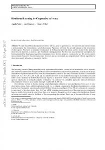
Figure 1.1 – A Venn diagram shows the position of Sum-Product Networks within the space of possible functions and distributions.

The Venn diagram in Figure 1.1 visualizes the relationship between ACs, SPNs, PGMs, compactly represented PGMs, tractable PGMs, valid ACs, valid SPNs, and low treewidth PGMs. Compactly represented PGMs are the family of PGMs where the representation size is polynomial in the number of variables. Tractable PGMs are the family of PGMs where the time of inference is polynomial in the number of variables. ACs and SPNs can be used to represent any arbitrary function; hence, the space of possible ACs and SPNs is a superset of the space of possible PGMs. Most PGMs can be compactly represented, but only a subset of these are tractable. The notion of valid ACs and valid SPNs refers to subsets of ACs and SPNs that encode proper distributions. Since inference is tractable in low-treewidth PGMs, valid ACs and valid SPNs subsume this type of models and also include other type of PGMs where inference is tractable.

4

1.1. Uncertainty in Dynamic Settings

1.1

Uncertainty in Dynamic Settings As mentioned above, uncertainty problems have different properties. One of the common

properties of uncertainty problems is being dynamic. In a dynamic setting the number of variables is not fixed and not known a priori. Consider for example a model that maps frames of YouTube videos to sequences of labels that describe the frames. Each frame can have a fixed number of variables that describe it (e.g., a variable for each pixel), but the number of frames varies from one YouTube video to another. Textual documents are usually treated as bags of words, but they can also be treated as sequences of words; also here the length of the sequence varies for each document. A naive approach to deal with this problem is to define an upper bound for the number of variables N , presumably based on the longest sequence that we have in a training set. Then, learn a fixed model with that number of variables. This approach suffers from two main problems. First, the resulting model will not be suitable for any sequence that is longer than N . Second, if the sequences in the training set are mostly shorter than N , we will end up having difficulties learning a correct model for the variables at the end, due to the shortage of data. The previous approach completely ignores the dynamic nature of the problem and treats it as if it was a static problem. The other way to deal with this type of problems is to focus on capturing the dynamics of the problem, i.e., how the variables at each time step interact and how they affect the variables on the next time step. By focusing on these two things, we can effectively and compactly capture the dynamic nature of the problem. The type of PGMs that is designed for dynamic uncertainty problems is called Dynamic PGMs and they are usually defined by specifying the interaction among the variables within each time step and between the time steps. Unfortunately, Dynamic PGMs exhibit the same intractability issues as regular PGMs. 5

1.2. Uncertainty in Online Settings

In this thesis, I present a new tractable probabilistic graphical model called Dynamic SumProduct Networks (DynamicSPN) that tackles the intractability problem in Dynamic PGMs by directly learning template SPNs that effectively and compactly capture the dynamic nature of a problem from sequence data that can possibly be of varying length. As in the case of SPNs, exact inference in DynamicSPNs is always tractable and can be done in a time that is linear in the size of the template SPNs. As part of the DynamicSPNs’ formulation, I introduced a new property, named invariance, that can be used to easily ensure that the DynamicSPN is valid (complete and decomposable). By exploiting this property, I also developed an iterative anytime search-and-score structure learning algorithm for DynamicSPNs that can learn the structure of a template SPN directly from data.

1.2

Uncertainty in Online Settings Another common property of uncertainty problems that has been gaining even more popu-

larity over the past several years is being online. In the online setting, the data is streamed into the model and the model has to update its belief incrementally. It is normal in this setting to assume that the model has only one chance to handle each data instance that appears in the stream. This means that many of the learning algorithms that perform multiple passes over the data during the learning process are not suitable for this type of settings. One paradigm that lends itself naturally to online settings is called Bayesian learning. It allows us to express prior knowledge about the model. Then, it updates the model after processing each data instance. Bayesian learning is mathematically elegant and very simple, but in most cases it is computationally hard. Previous work A. Rashwan (2016) proposes the use of an approximation technique called moment matching to develop a Bayesian learning algorithm for SPNs, where the focus was on

6

1.3. Decision Making under Uncertainty

learning the joint distribution over random variables. This type of learning that focuses on the joint distribution is called generative learning. In this thesis, I developed a new learning algorithm called DiscBays for a special type of SPNs that has no latent variables. DiscBays is an online algorithm that utilizes the Bayesian learning paradigm. It directly learns a conditional distribution of a target variable given another set of variables. This type of learning is known as discriminative learning. Unfortunately, the moment matching technique is not feasible in the discriminative case. Instead, I developed a novel approximation technique based on mode matching that and works nicely for the discriminative case.

1.3

Decision Making under Uncertainty The notion of intelligent agents is yet another concept that is at the heart of AI. Agents are

entities that have some perceptions about the environment and they can act upon it, where acting involves making decisions. Besides random variables, decision making problems often require two additional types of variables: decision and utility variables. Decision variables encode the possible actions an agent can take and utility variables encode the desirability of the possible outcomes. A main concern in AI is to develop what is known as rational agents. An agent is considered rational if it follows a set of axioms, named axioms of rationality; these axioms impose constraints on how to define the agent’s utility. A rational agent is also defined as an agent that follows the maximum expected utility principle, which states that the agent should always take the actions that maximize its expected utility. Influence diagrams (also known as decision networks) are a class of PGMs that concerns the problem of decision making under uncertainty. They provide a framework to define decision problems using three types of nodes: chance, decision, and utility nodes, where chance nodes correspond to random variables.

7

1.4. Summary of the Contributions This thesis presents a new model called DecisionSPMN, which is an extension of SPNs to the class of decision making problems. To enable this, the new model introduces two new types of nodes: max nodes to represent the maximization operation over different possible values of a decision variable, and utility nodes to represent the utility values. The solution of a DecisionSPMN is the set of decisions that maximizes the expected utility and it can be computed in a time that is linear in the size of the network. The semantics of the max node is that its output is the value of the decision that leads to the maximal value among all decisions. Analogously to sum-product networks, I introduce a set of properties that guarantee the validity of the DecisionSPMN, such that the solution of a DecisionSPMN will correspond to the expected utility obtained from a valid embedded probabilistic model and a utility function that are encoded by the network.

1.4

Summary of the Contributions Using the idea of modeling inference, I developed two new probabilistic graphical models

that guarantee tractable exact inference. I also developed a new online discriminative Bayesian parameter learning algorithm for a special class of tractable models called Selective Sum-Product Networks based on the novel idea of Bayesian mode matching. The following list summarizes the contributions made in this thesis:

• Dynamic Sum-Product Networks (DynamicSPNs): I developed a new tractable exact inference model called: Dynamic Sum-Product Networks (DynamicSPNs), that is suitable for sequence data of varying length. I introduced the concept of template networks that can be repeated to model data sequences of any

8

1.5. Thesis Structure length. I also introduced a new property: invariance, which can be used to easily ensure that the DynamicSPNis valid (complete and decomposable) • A Structure Learning Algorithm for DynamicSPNs (LearnDynamicSPN): I developed an iterative anytime search-and-score structure learning algorithm for DynamicSPNs that can learn the structure of a template network directly from data. • A Discriminative Bayesian Learning Algorithm for Selective SPNs (DiscBays): I developed a new online discriminative Bayesian learning technique for a special class of tractable models called Selective Sum-Product Networks based on the novel idea of Bayesian mode matching. This new technique can be used when data is presented in an online fashion and can easily be extended to a distributed learning setting. • Decision Sum-Product Networks (DecisionSPMN): I developed a new tractable model for decision problems, named DecisionSPMN. This model adds two new types of nodes to SPNs: max nodes and utility nodes. Optimal decision strategies can be obtained from DecisionSPMN in time that is linear in the size of the network. • Structure and Parameter Learning for DecisionSPMNs (LearnDecisionSPMN): I developed algorithms to learn both the structure and the parameters of decision problems directly from data. The structure learning algorithm is recursive and respects the constraint imposed by the decision problem’s partial order.

1.5

Thesis Structure The thesis is structured as follows: 9

1.5. Thesis Structure

• Chapter 2 The background materials that are needed for the rest of the thesis are presented in this chapter. The chapter introduces two of the traditional probabilistic graphical models (PGMs): Bayesian networks and Markov networks. Then, after introducing the concept of network polynomial functions, the chapter explains SPNs, how to learn them, and how to do inference with them. • Chapter 3 This chapter presents Dynamic Sum-Product Networks (DynamicSPNs). It also presents an invariance property that is sufficient to ensure that the resulting DynamicSPN is valid (i.e., encodes a joint distribution) by being complete and decomposable. The chapter also presents a general anytime search-and-score framework with a local search technique to learn the structure of a template network that defines a DynamicSPN based on data sequences of varying length. The experimental results section in this chapter demonstrates the advantages of DynamicSPNs over static SPNs, Dynamic Bayesian Networks, and Hidden Markov Models on synthetic and real sequence data. • Chapter 4 This chapter presents a new online discriminative Bayesian learning algorithm called DiscBays for Selective Sum-Product Networks (SSPNs). After discussing SSPNs and the previous work on discriminative and Bayesian learning for SPNs, the chapter presents DiscBays and provides a brief discussion of how to use it in a distributed fashion. The experimental section shows the results when comparing DiscBays to generative and (nonBayesian) discriminative learning algorithms. • Chapter 5 10

1.5. Thesis Structure The new tractable model for decision making, DecisionSPMN, is presented in this chapter. The chapter discuss the relationship between DecisionSPMN and some other related works. The formulation of DecisionSPMN along with the algorithms for learning the structure and the parameters are presented in this chapter. • Chapter 6 This concluding chapter provides a summary of the thesis and a discussion of possible future directions.

11

Chapter 2 Background This chapter starts by introducing two of the traditional probabilistic graphical models (PGMs): Bayesian networks and Markov networks. Section 2.2 explains how we can construct a function called network polynomial that encodes a joint distribution. Section 2.3 presents Sum-Product Networks (SPNs), which emerged recently as a new class of tractable probabilistic graphical models, that are built upon the idea of network polynomials and guarantee linear time inference in the size of the network.

2.1

Probabilistic Graphical Models PGMs are a powerful and an elegant framework for modeling uncertainty by utilizing prob-

ability theory and graph theory. Generally, a PGM G over a set of random variables X = {X1 , X2 , ..., XN } is defined using a graph G = hV, Ei and a set of non-negative functions F, where V is a set of nodes, E is a set of edges such that E ⊆ V × V ; each node n ∈ V is associated with a random variable. The set of functions F factorizes the joint distribution according

12

2.1. Probabilistic Graphical Models to the conditional independence constraints induced by the graph G. G is called the structure of the PGM and F is its parameterization. If G is a directed acyclic graph (DAG), which means that all edges are directed and the graph contains no cycles, and each fn ∈ F is a conditional distribution of variable Xn given its parents, i.e fn (Xn , parents(Xn )) = Pr(Xn |parents(Xn )), then G is called a Bayesian Network (also known as Bayes Net and Belief Network). Definition 2.1 (Bayesian Networks) A Bayesian network B over a set of random variables X = {X1 , X2 , ..., XN } is a pair B = hG, Fi, where G = hV, Ei is a directed acyclic graph, and F is a set of conditional probability distributions. Each node n ∈ V is associated with a random variable and each function fn ∈ F is a conditional distribution of the variable Xn given its parents fn (Xn , parents(Xn )) = Pr(Xn |parents(Xn )). The joint distribution of X is factorized as:

Pr(X0 , X1 , ..., XN ) =

Y

Pr(Xn |parents(Xn ))

n∈V

Figure 2.1 shows simple examples of Bayesian networks, (a) is the burglar alarm Bayesian network, in which an alarm has a possibility of being set off by either a burglary or an earthquake and there is a possibility of receiving a call from two of the neighbors if they heard the alarm; (b) is known as the sprinkler network and shows the relationship among five random variables: season of the year, state of the sprinkler, whether it is raining, whether the grass is wet, and whether the grass is slippery. In the case where G is an undirected graph and the joint distribution is factorized according to the cliques of G, the PGM G is called a Markov Network or a Markov random field. More 13

2.1. Probabilistic Graphical Models formally, let C be the set of all maximal cliques of G and for each clique C ∈ C we associate a non-negative function fC ∈ F : Val(C) → R+ , where Val(C) is the Cartesian product of the state spaces of the random variables that are in clique C. These functions are called factors. Definition 2.2 (Markov Networks) A Markov network M over a set of random variables X = {X1 , X2 , ..., XN } is a pair M = hG, Fi, where G = hV, Ei is an undirected graph, and F is a set of factors defined over the maximal cliques of the graph fC ∈ F : Val(C) → R+ . The joint distribution of X is factorized as:

Pr(X0 , X1 , ..., XN ) =

1 Y fC (Xc ), Z C∈C

where Z is a normalization constant. If a PGM encodes all and only the conditional independence constraints of a distribution, then it is called a perfect map of that distribution. Bayesian networks and Markov networks can equivalently be perfect maps for some distributions, but there are also distributions that can only be modeled using one of these two representations Koller and Friedman (2009). Figure 2.2 shows two Markov networks structures, (a) is an example of a Markov network that encodes conditional independence constraints that can not be perfectly modeled using a Bayesian network (any Bayesian network will have either less or more conditional independence assertions); (b) is an example of a grid structure that is widely used in many computer vision and image processing applications Wang et al. (2013).

14

2.1. Probabilistic Graphical Models

Season

Burglary

Earthquake

Sprinkler

Alarm

JohnCalls

Rain

WetGrass

MaryCalls

Slippery

(a)

(b)

Figure 2.1 – Examples of Bayesian networks Pearl (1995); Koller and Friedman (2009). Each node is associated with a random variable and a conditional probability distribution. (a) is the burglar alarm Bayesian network. (b) is known as the sprinkler network.

2.1.1

Inference in Probabilistic Graphical Models

Inference in PGMs is the task of answering probabilistic queries, such as the marginal probability of some variables Y, i.e. Pr(Y), or the conditional probability of some variables Y given the values of other variables E, i.e., Pr(Y|E), where E is usually called the evidence. Both exact and approximate inference are known to be computationally hard, where the former is #P-Hard and the later is NP-hard Valiant (1979); Dagum and Luby (1993). Exact inference in PGMs can be done using the variable elimination algorithm. Other exact inference algorithms, such as junction trees and the Cutset-conditioning algorithm can be seen as variants of the variable elimination algorithm. The next example demonstrates how the algorithm works using a small concrete example.

15


X0

X1

X2

X3

X0

X4

X8

X12

X1

X5

X9

X13

X2

X6

X10

X14

X3

X7

X11

X15

(a)

(b)

Figure 2.2 – Examples of two Markov network structures, (a) is an example of a Markov network that encodes conditional independencies that can not be perfectly modeled using a Bayesian network (any Bayesian network will have either less or more conditional independence assertions); (b) is an example of a grid structure that is widely used in many computer vision and image processing applications Wang et al. (2013).

Example 2.1 (Variable Elimination Algorithm) Consider the Bayesian networks in Figure 2.3. The network has m + 1 binary random variables. Each variable is represented by a node in the graph and edges correspond to dependencies between the variables. Assume that we want to compute the marginal probability of X1 = T rue, i.e Pr(X1 = True). One way to compute the marginal is by enumerating the entire joint distribution and summing the entries that are consistent with X1 = T rue:

Pr(X1 = True) =

XXX Y

X2 X3

...

X Xm

Pr(X1 = True, Y, X2, X3, ..., Xm ) {z } | A

Each term A in the summation is an entry in the joint distribution, which is in this case

16


Y

X1

X2

X3

...

Xm

Figure 2.3 – An example Bayesian network with m + 1 variables. Each variable is represented by a node in the graph and edges correspond to dependencies between the variables. This structure is also known as the Naive Bayes model. a giant table with 2m+1 entries. We can exploit the structure of the Bayesian network to substitute the term A with the small factored Conditional Probability Tables (CPTs) that are associated with the nodes in the Bayesian network:

Pr(X1 = True) =

XXX

=

XXX

Y

Y

...

X

...

X

X2 X3

X2 X3

Pr(Y)Pr(X1 = True|Y)Pr(X2 |Y)Pr(X3 |Y)...Pr(Xm |Y)

Xm

f0 (Y)f1 (X1 = True, Y)f2 (X2 , Y)f3 (X3 , Y)...fm (Xm , Y)

Xm

In the second step we used the notation fi (X), where X can be a set of variables, to denote a tabular representation of the CPTs; fi (X) is called a factor and X is its scope. To efficiently compute the previous equation we can utilize the dynamic programming technique by pushing the sums inside the product and store the intermediate results in new temporary factors.

17


Pr(X1 = True) =

X

f0 (Y)f1 (X1 = True, Y)

Y

X

f2 (X2 , Y)

X2

X

f3 (X3 , Y)...

X3

X |

| |

fm (Xm , Y)

Xm

{z

fm+1 (Y)

{z

fj (Y)

{z

fk (Y)

Each new intermediate factor is the result of summing out a variable after multiplying all the factors that include the variable in their scopes. The factor multiplication operation is a binary operation that takes two factors fi (X) and fj (Y) and returns a new factor that has a scope of X ∪ Y. The order in which the summations are performed is called the elimination order. In the previous example the order was: Xm , Xm−1 , ..., X3 , X2 , Y . The elimination order has a large impact on the efficiency of the variable elimination algorithm. This is mainly due to two related facts: 1) the factor multiplication operation returns a new factor with a scope that is the union of its operands’ scopes, 2) a tabular representation for factors is exponential in the size of its scope. So, while one elimination order can be very efficient, another one might produce intractable intermediate factors. In the previous example, each elimination step other than the last one produces a new intermediate factor with scope {Y } and each multiplication is between two factors, one with the scope {Xi , Y }, i ∈ 1, ..., m and the other with the scope {Y }. Hence, the largest produced factor has a scope of size 2. Now let us look into an example where an inefficient elimination order is used: Example 2.2 (Inefficient Elimination Order) Consider the same Bayesian network and the same probabilistic query as in Example 2.1. If

18

} } }

2.1. Probabilistic Graphical Models we perform variable elimination using the elimination order Y, Xm , Xm−1 , ..., X3 , X2 we will get the following:

Pr(X1 = True) =

XX X2 X3

...

XX Xm

f0 (Y)f1 (X1 = True, Y)f2 (X2 , Y)f3 (X3 , Y)...fm (Xm , Y)

|Y

{z

fm+1 (X1 ,X2 ,X3 ,...,Xm )

The resulting intermediate factor fm+1 has the scope of X1 , X2 , X3 , ..., Xm and requires O(2m ) space for its representation. For some special structures the optimal elimination order is known. For example, if the structure is a polytree, an optimal elimination order consists of eliminating singly connected nodes first. However, for arbitrary structures, finding the optimal elimination order is an NP-Hard problem. The variable elimination algorithm is outlined in Algorithm 2.1. It takes as inputs a set of factors F and an ordered set O of the variables. The algorithm iterates over O and for each v ∈ O it constructs a new factor by multiplying all the factors that involve v, summing out the variable v, then remove all the factors that involve v from F. Algorithm 2.1: Variable Elimination Input: F: Set of local probablistic models O: Elimination order foreach v ∈ O do relatedF ← {f ∈ F : v ∈ Scope(f)}; otherF ← − relatedF; PF Q newf ← v f ∈relatedF f ; F ← otherF ∪ {newf}; Q return f ∈F f

19

}

2.2. Network Polynomials

A

B

C

A a a ¯

ΘA θa θa¯

(a)

A a a a ¯ a ¯

B b ¯b b ¯b

ΘB|A θb|a θ¯b|a θb|¯a θ¯b|¯a

A a a a ¯ a ¯

C c c¯ c c¯

ΘC|A θc|a θc¯|a θc|¯a θc¯|¯a

(b)

Figure 2.4 – The Bayesian network that is used in Example 2.3, (a) shows the structure of the network, and (b) the conditional probability tables for the variables A, B, and C from left to right.

2.2

Network Polynomials

A network polynomial Darwiche (2000) is a function that encodes a joint distribution such that it can be evaluated in order to answer probabilistic queries. The next example demonstrates this idea by showing a function that encodes the joint distribution of three variables. Example 2.3 (A Function That Encodes A Joint Distribution) Consider the Bayesian network in Figure 2.4. The network has three binary random variables. The figure shows the structure and also shows the conditional probability tables for the three variables. We used the notation x and x¯ to denote the true and false values of variable X, respectively. The joint distribution table is the result of the Cartesian product of the three conditional probability tables:

20


A

B

C

P (A, B, C)

a

b

c

θa · θb|a · θc|a

a

b

c¯

θa · θb|a · θc¯|a

a

¯b

c

θa · θ¯b|a · θc|a

a

¯b

c¯

θa · θ¯b|a · θc¯|a

a ¯

b

c

θa¯ · θb|¯a · θc|¯a

a ¯

b

c¯

θa¯ · θb|¯a · θc¯|¯a

a ¯

¯b

c

θa¯ · θ¯b|¯a · θc|¯a

a ¯ ¯b c¯ θa¯ · θ¯b|¯a · θc¯|¯a For each variable we can introduce two indicators Ix and Ix¯ , where every indicator can take either the value of 1 or 0. Using these indicators we can write a function that encodes the joint distribution table as follows:

f = Ia · Ib · Ic · θa · θb|a · θc|a + Ia · Ib · Ic¯ · θa · θb|a · θc¯|a + Ia · I¯b · Ic · θa · θ¯b|a · θc|a + Ia · I¯b · Ic¯ · θa · θ¯b|a · θc¯|a (2.1) + Ia¯ · Ib · Ic · θa¯ · θb|¯a · θc|¯a + Ia¯ · Ib · Ic¯ · θa¯ · θb|¯a · θc¯|¯a + Ia¯ · I¯b · Ic · θa¯ · θ¯b|¯a · θc|¯a + Ia¯ · I¯b · Ic¯ · θa¯ · θ¯b|¯a · θc¯|¯a

21


+

×

θa

θb|a

θc|a

a

×

b

c

θa

θb|a

θc̄|a

a

×

b

θā

c̄

θb�|a

θc|a

×

ā

b�

c

θā

θb�|a

...

θc̄|a

ā

b�

c̄

Figure 2.5 – An arithmetic circuit of the function in Equation 2.1 The previous function was obtained by multiplying each row in the probability table of the joint distribution with the indicators that are consistent with the row. To use the previous function for inference, we can simply replace each indicator with the value of the evidence. For example, if we want to compute P (a, b, c¯) we will set Ia , Ib , and Ic¯ to 1 and set all the other indicators to 0. The result after evaluating the function will be θa ·θb|a ·θc¯|a , which is the probability of the assignment according to the Bayesian network. The function in Equation 2.1 can be graphically represented using an arithmetic circuit as shown in Figure 2.5. A multi-linear function that encodes a joint distribution, similar to the one in Equation. 2.1, is called a network polynomial Darwiche (2003). Darwiche shows that many probabilistic queries can be obtained in a time that is linear in the size of the network polynomial by evaluating the network polynomial or evaluating its partial derivatives with respect to the indicators. However, the size of the network polynomial itself will grow exponentially in the number of variables if it was constructed naively as in the previous example. In the same work, Darwiche proposes the use of arithmetic circuits as a graphical representation of the network polynomial. He also proposes the use of the junction tree algorithm as a mean to construct compact arithmetic circuits. This process is known in the literature as compilation. Although this process can produce arithmetic circuits that are more compact than those obtained by straight forward evaluation, it suffers from two major drawbacks. First, it assumes that the structure and the parameters are known. Second, the compilation process has an exponential time and space complexity in the size of the cliques

22

2.3. Sum-Product Networks

of the junction tree; hence, it is prone to becoming intractable. A method that focuses on learning arithmetic circuits directly from data was developed in Lowd and Domingos (2012). The method is based on the search-and-score technique, with a score function that prefers compact models by penalizing models that have more edges. The method avoided the need to compile the Bayesian network for each candidate structure by incrementally building the arithmetic circuit.

2.3

Sum-Product Networks

Sum-product networks (SPN) Poon and Domingos (2011) have recently emerged as a new class of tractable probabilistic graphical models. Unlike Bayesian and Markov networks where inference may be exponential in the size of the network as shown above, inference in SPNs is linear in the size of the network. Also, contrary to Bayesian networks and Markov networks where we have separate representations and inference algorithms, SPNs can be seen as both graphical representations and inference machines at the same time. An SPN is defined using a rooted DAG whose internal nodes are either sum or product nodes, and the leaves are indicators of the random variables. Each child of a sum node has an associated weight. Definition 2.3 (Sum-Product Network Poon and Domingos (2011)) A sum-product network (SPN) over n binary variables X1 , ..., Xn is a rooted directed acyclic graph whose leaves are the indicators Ix1 , ..., Ixn and Ix¯1 , ..., Ix¯n , and whose internal nodes are sums and products. Each edge (i, j) emanating from a sum node i has a non-negative weight, wij . The value of a product node is the product of the P values of its children. The value of a sum node is j∈Ch(i) wij vj , where Ch(i) is the

23

2.3. Sum-Product Networks set of children of i and vj is the value of node j. The value of an SPN is the value of its root. The scope of a node is the set of variables that appear in the sub-SPN rooted at that node. The scope of a leaf node is the variable that the indicator refers to and the scope of an interior node is the union of the scopes of its children. The value of an SPN could be seen as the output of a network polynomial whose variables are the indicator variables and the coefficients are the weights Darwiche (2003). This polynomial represents a joint probability distribution over the variables involved if the SPN satisfies the following two properties Poon and Domingos (2011): Definition 2.4 (Completeness Poon and Domingos (2011)) An SPN is complete iff all children of the same sum node have the same scope, where the scope is the set of variables that are included in a child.

Definition 2.5 (Decomposability Poon and Domingos (2011)) An SPN is decomposable iff no variable appears in more than one child of a product node. An SPN that is both complete and decomposable is valid, and it correctly computes a joint distribution over the variables in its scope. The next example shows several basic distributions represented as SPNs. Example 2.4 (Basic distributions encoded as SPNs) Several basic distributions are encoded by SPNs exhibiting simple structures. For instance, a univariate distribution can be encoded using an SPN whose root node is a sum that is linked to each indicator of a single variable X (see Fig. 2.6(a)). A factored distribution over a set of

24

2.3. Sum-Product Networks variables X1 , ..., Xn is encoded by a root product node linked to univariate distributions for each variable Xi (see Fig. 2.6(b)). A naive Bayes model is encoded by a root sum node linked to a set of factored distributions (see Fig. 2.6(c)).

2.3.1

Inference in Sum-Product Networks

Inference about the joint probability of the variables in the scope of an SPNs can be answered by replacing the indicators with either 0 or 1 then perform a bottom up pass. If the value of a variable X = True, then we set the corresponding indicator Ix = 1 and the other indicator Ix¯ = 0. If X = False, then we set Ix = 0 and Ix¯ = 1. If we want to marginalize out a variable X, then we set Ix = 1 and Ix¯ = 1. Conditional inference queries Pr(X = x|Y = y) can be answered by taking the ratio of the values obtained by two bottom up passes of an SPN. In the first pass, we initialize Ix = 1, Ix¯ = 0, Iy = 1, Iy¯ = 0 and set all remaining indicators to 1 in order to compute a value proportional to the desired query. In the second pass, we initialize Iy = 1, Iy¯ = 0 and set all remaining indicators to 1 in order to compute the normalization constant. The linear complexity of inference in SPNs is an appealing property given that inference for other models such as Bayesian networks is exponential in the size of the network in the worst case.

2.3.2

Learning Sum-Product Networks

Poon and Domingo Poon and Domingos (2011) propose two algorithms to directly learn the parameters of SPNs from data: expectation-maximization and gradient descent. The expectationmaximization algorithm relies on interpreting the sum nodes as latent random variables. The gradient descent algorithm uses the partial derivatives of the network polynomial encoded by

25


the SPN. These partial derivatives can easily be obtained by performing a bottom-up pass followed by a top-down pass, where in the first pass we perform inference as described in the previous subsection and in the second pass we apply the chain rule of derivatives. A discriminative parameter learning algorithm has been proposed in Gens and Domingos (2012) and a Bayesian learning algorithm has also been recently proposed in A. Rashwan (2016). A discussion about these two algorithms is presented in Section 4.2. Several algorithms have been proposed to learn the structure of SPNs Rooshenas and Lowd (2014); Gens and Domingos (2013). In Section 5.4.1 we develop a structure learning algorithm that generalizes LearnSPN() to decision problems. LearnSPN() is a recursive top-down structure learning algorithm for SPNs. Given a dataset, LearnSPN() tries first to partition the random variables into independent subsets using an independence statistical test, such as χ2 or G-test. If such a partitioning is found, the algorithm introduces a product node, where each child of the product node correspond to one of the found subsets. If no independent subsets are found, the algorithm introduces a sum node and clusters the dataset into similar instances; each cluster will be associated with one of the sum node’s children. The algorithm recursively repeats these steps until only one variable is left in the dataset, at which point it introduces a univariate distribution over that variable.

26


×

+

+ Ix

I x̄

+

+

Ix Ix̄ Iy Iȳ Iz Iz̄

(a)

(b)

+

+

+

×

×

+

+

+

+

Ix Ix̄ Iy Iȳ Iz Iz̄ (c)

Figure 2.6 – Basic distributions encoded as SPNs. (a) shows an SPN that encodes a univariate distribution over a binary variable x. (b) shows an SPN that encodes factored distribution over three binary variables x, y, and z. (c) is an SPN that encodes a naive Bayes model over three binary variables x, y, and z. The root sum node corresponds to a the hidden class variable.

27

Chapter 3 Dynamic Sum-Product Networks

3.1

Introduction This chapter presents Dynamic Sum-Product Networks (DynamicSPNs), an extension to

SPNs that model sequence data of varying length. The time for inference in DynamicSPNs is guaranteed to always be linear in the size of the network even if some or all the random variables were not observed. Similar to Dynamic Bayesian networks (DBNs) Dean and Kanazawa (1989); Murphy (2002), DynamicSPNs consist of a template network that repeats as many times as the length of a data sequence. I describe an invariance property for the template network that is sufficient to ensure that the resulting DynamicSPN is valid (i.e., encodes a joint distribution) by being complete and decomposable. Since existing structure learning algoritms for SPNs assume a fixed set of variables and fixed-length data, they cannot be used to learn the structure of a DynamicSPN. This chapter presents a general anytime search-and-score framework with a specific local search technique to learn the structure of the template network that defines a DynamicSPN based on data sequences of varying length. I demonstrate the advantages of DynamicSPNs over

28

3.2. Related Models

static SPNs, DBNs, and HMMs with synthetic and real sequence data.

3.2

Related Models

3.2.1

Dynamic Arithmetic Circuits

An extension to network polynomials for DBNs was given in Brandherm and Jameson (2004). The proposed procedure compiles a DBN into a recursive network polynomial, where each network polynomial for time step t is a function of the network polynomial of time step t − 1. The output of each time step’s network polynomial is a table over the Cartesian product of the values of the variables in the belief state (the nodes at time step t − 1 that are parents of nodes at time step t). The recursive network polynomial can, essentially, be obtained by performing variable elimination with a specified order on the DBN. The recursive network polynomial can be represented with a special AC that has multiple roots and placeholders to plug the roots of the previous time step’s network polynomial. I call this representation Dynamic Arithmetic Circuits (Dynamic ACs). Dynamic ACs are compiled representations, which means that we have to start from a known DBN and then convert it to a Dynamic AC. There is a risk that the compiled Dynamic AC will be intractable because of the the size of the output table or the internal representation. For the output table, the authors proposed to use the Boyen-Koller Boyen and Koller (1998) method to approximate the large output table with several smaller ones. The internal representation, on the other hand, may still suffer of an exponential blow up since it depends on the variable elimination order and have the same complexity as the variable elimination algorithm. Thus, compiling a DBN to a Dynamic AC does not reduce the complexity of inference, but only makes it linear in the size of the compiled Dynamic AC, which could be intractable. In this

29

3.2. Related Models

work I present a model that can be learned directly from data and present a structure learning algorithm that guarantees to find tractable models.

3.2.2

Dynamic Bayesian Networks

As we have seen in Section 2.1, Bayesian networks are defined over a fixed number of variables. Dynamic Bayesian Networks (DBNs) extend Bayesian networks to the dynamic setting by defining a template structure that can be instantiated for sequences of varying lengths Murphy (2002); Koller and Friedman (2009). A DBN is defined as a pair hB1 , B→ i, where B1 is a Bayesian network that defines the initial distribution, and B→ is a two-time-slice Bayesian network (2TBN) that defines the conditional distribution of the random variables at time step t given the variables at time step t − 1. Parameters learning in DBNs can be done by tying the parameters across time slices. REVEAL Liang et al. (1998) is a greedy search-and-score structure learning algorithm for DBNs that focuses on capturing the dynamics of the variables between the time steps. Given a data instance of length T , inference can be done by unrolling the DBN for T time slices. The unrolled version is a regular Bayesian networks; hence, we can use any of the inference algorithms for Bayesian networks. The problem with this approach is of two folds. First, T can be arbitrarily large, which would make the unrolled Bayesian network large as well. Second, common inference tasks in DBNs require maintaining a belief state over time, which is a distribution over the variables at time step t given all the previous observations. The exact representation of the belief state is exponentially large in the number of hidden variables. Some inference algorithms, such as Boyen-Koller Boyen and Koller (1998) and the factored frontier algorithm Murphy and Weiss (2001), tackle this problem by approximating the belief state using a product of marginals of some cluster of variables.

30

3.3. Dynamic Sum-Product Networks

3.3

Dynamic Sum-Product Networks Sequence data such as time series data is typically generated by a dynamic process. Such data

is conveniently modeled using structure that may be repeated as many times as the length of the process and a way to model the dependencies between the repeated structure. In this context, we propose dynamic SPNs (DynamicSPNs) as a generalization of SPNs for modeling sequence data of varying length. This is motivated by the fact that if a DynamicSPN is a valid SPN, then inference queries can be answered in linear time thereby providing a way to perform tractable inference on sequence data. As an example, consider temporal sequence data that is generated by n variables (or features) over T time steps:

D

hX1 , X2 , . . . , Xn i1 , hX1 , X2 , . . . , Xn i2 , . . . , hX1 , X2 , . . . , Xn iT

E

where Xi , i = 1 . . . n is a random variable in one time slice and T may vary with each sequence. Note that non-temporal sequence data such as sentences (sequence of words) can also be represented by sequences of repeated features. We will label the set of repeating variables as a slice and we will index slices by t even if the sequence is not temporal, for uniformity. A DynamicSPN models sequences of varying length with a fixed number of parameters by using a template that is repeated at each slice. This is analogous to DBNs where the template corresponds to the network that connects two consecutive slices. We define the template SPN for each slice hX1 , X2 , . . . , Xn iT as follows.

31


Definition 3.1 (Template network) A template network for a slice of n binary variables at time t, hX1 , X2 , . . . , Xn it , is a directed acyclic graph with k roots and k + 2n leaf nodes. The 2n leaf nodes are the indicator variables, Ixt1 , Ixt2 , . . . , Ixtn , Ix¯t1 , Ix¯t2 , . . . , Ix¯tn . The remaining k leaves and an equal number of roots are interface nodes to and from the template for the previous and next slices, respectively. The interface and interior nodes are either sum or product nodes. Each edge (i, j) emanating from a sum node i has a non-negative weight wij as in a SPN. Furthermore, we define a bijective mapping f between the input and output interface nodes. A generic template network is shown in Fig. 3.1.

×

×

+

+

+

+

+

+

+

+

×

×


Figure 3.1 – An example of a generic template network. Notice the interface nodes in red.

In addition to the above, we define two special networks.

32


Definition 3.2 (Bottom network) A bottom network for the first slice of n binary variables, hX1 , X2 , . . . , Xn i1 , is a directed acyclic graph with k roots and 2n leaf nodes. The 2n leaf nodes are the indicator variables, Ix11 , Ix12 , . . . , Ix1n , Ix¯11 , Ix¯12 , ..., Ix¯1n . The k roots are interface nodes to the template network for the next slice. The interface and interior nodes are either sum or product nodes. Each edge (i, j) emanating from a sum node i has a nonnegative weight wij as in a SPN.

Definition 3.3 (Top network) Define a top network as a rooted directed acyclic graph composed of sum and product nodes with k leaves. The leaves of this network are interface nodes, which were introduced previously. Each edge (i, j) emanating from a sum node i has a non-negative weight wij as in a SPN. A DynamicSPN is obtained by stacking as many copies of the template network of Def. 3.1 as the number of slices in a sequence less 1 on top of a bottom network. This is capped by a top network. Two copies of the template are stacked by merging the input interface nodes of the upper copy with the output interface nodes of the lower copy. A template is stacked on a bottom network by merging the output interface nodes of the bottom network with the input interface nodes of the template. Analogously, the top network is stacked on a template by merging the input interface nodes of the top network with the output interface nodes of the template. Figure 3.2 shows an example with 3 slices of 2 variables each. While a DynamicSPN conforms to the structure required of a SPN, we note that the bottom, template and top networks are not SPNs when considered separately. The bottom and

33


+ ×

×

+

+

+

+

+

+

+

+

×

×

Ix,2

Ix,2

Iy,2

Iȳ,2

Iz,2

Iz,2

+

+

+

+

+

+

+

+

×

×

Ix,1

Ix,1

Iy,1

Iȳ,1

Iz,1

Iz,1

+

+

+

+

+

+

Ix,0

Ix,0

Iy,0

Iȳ,0

Iz,0

Iz,0

Figure 3.2 – A generic example of a complete DynamicSPN unrolled over 3 time slices. Template network is stacked on the bottom network and capped by the top network.

template networks have multiple roots while an SPN has a single root. The template and top networks also have leaves that are not indicator variables while all the leaves of an SPN are indicator variables. As we mentioned previously, completeness and decomposability are sufficient to ensure the validity of an SPN. While one could check that each sum node in the DynamicSPN is complete

34

3.3. Dynamic Sum-Product Networks and each product node is decomposable, we provide a simpler way to ensure that any DynamicSPN is complete and decomposable. In particular, we describe an invariance property for the template network that can be verified directly in the template without unrolling the DynamicSPN. This invariance property is sufficient to ensure that completeness and decomposability are satisfied in the DynamicSPN for any number of slices. Definition 3.4 (Invariance) A template network over hX1 , ..., Xn it is invariant when the scope of each input interface node excludes variables {X1t , ..., Xnt } and for all pairs of input interface nodes, i and j, the following properties hold: • scope(i) = scope(j) ∨ scope(i) ∩ scope(j) = ∅ • scope(i) = scope(j) ⇐⇒ scope(f (i)) = scope(f (j)) • scope(i)∩scope(j) = ∅ ⇐⇒ scope(f (i))∩scope(f (j))=∅ • all interior and output sum nodes are complete • all interior and output product nodes are decomposable Here f is the bijective mapping that indicates which input nodes correspond to which output nodes in the interface. Intuitively, a template network is invariant if we can assign a scope to each input interface node such that each pair of input interface nodes have the same scope or disjoint scopes, and the same relation holds between the scopes of the corresponding output nodes. Scopes of pairs of corresponding interface nodes must be the same or disjoint because a product node is decomposable

35


when its children have disjoint scopes and a sum node is complete when its children have identical scope. Hence, verifying the identity or disjoint relation of the scopes for every pair of input interface nodes helps us in verifying the completeness and decomposability of the remaining nodes in the template. Note that the invariance property is only concerned with the validity of the resulting unrolled SPNs and it does not imply that the process is stationarity. Theorem 3.1 below shows that the invariance property of Def. .1 can be used to ensure that the corresponding DynamicSPN is complete and decomposable. Theorem 3.1 If (a) the bottom network is complete and decomposable, (b) the scopes of all pairs of output interface nodes of the bottom network are either identical or disjoint, (c) the scopes of the output interface nodes of the bottom network can be used to assign scopes to the input interface nodes of the template and top networks in such a way that the template network is invariant and the top network is complete and decomposable, then the corresponding DynamicSPN is complete and decomposable. Proof. Below, I sketch a proof by induction (see Appendix A for more details). For the base case, consider a single-slice DynamicSPN that contains the bottom and top networks only. The bottom network is complete and decomposable by assumption. Since the interface output nodes of the bottom network are merged with the input interface nodes of the top network, they are assigned the same scope, which ensures that the top network is also complete and decomposable. Hence a single-slice DynamicSPN is complete and decomposable. For the induction step, assume that a DynamicSPN of T slices is complete and decomposable. Consider a DynamicSPN of T + 1 slices that shares the same bottom network and the same first T − 1 copies of the template network as the DynamicSPN of T slices. Hence the bottom network and the first 36

3.4. Structure Learning of DynamicSPNs T − 1 copies of the template network in the DynamicSPN of T + 1 slices are complete and decomposable. Since the next copy of the template network is invariant when its input interface nodes are assigned the scopes with the same identity and disjoint relations as the scopes of the output interface nodes of the bottom network, it is also complete and decomposable. Similarly the top network is complete and decomposable since its interface nodes inherit the scopes of the interface nodes of the template network which have the same identity and disjoint relations as the output interface nodes of the bottom network. Hence DynamicSPNs of any length are complete and decomposable. In summary, a DynamicSPN is an SPN with a repeated structure and tied parameters specified by the template. The likelihood of a data sequence can be computed by instantiating the indicator variables accordingly and propagating the values to the root. Hence inference can be performed in linear time with respect to the size of the network.

3.4

Structure Learning of DynamicSPNs

As a DynamicSPN is an SPN, we could ignore the repeated structure and learn an SPN for the number of variables corresponding to the longest sequence. Shorter sequences could be treated as sequences with missing data for the unobserved slices. Unfortunately, this is intractable for very long sequences because the inability to model the repeated structure implies that the SPN will be very large and the learning computationally intensive. This approach may be feasible for datasets that contain only short sequences, nevertheless the amount of data needed may be prohibitively large because in the absence of a repeating structure the number of parameters is much higher. Furthermore, the SPN could be asked to perform inference on a sequence that is longer than any of the training sequences, and it is likely to perform poorly. 37

3.4. Structure Learning of DynamicSPNs

Alternately, it is tempting to apply existing algorithms to learn the repeated structure of the DynamicSPN. Unfortunately, this is not possible. As existing algorithms assume a fixed set of variables, one could break data sequences into fixed-length segments corresponding to each slice. An SPN can be learned from this dataset of segments. However, it is not clear how to use the resulting SPN to construct a template network because a regular SPN has a single root while the template network has multiple roots and an equal number of input leaves that are not indicator variables. One would have to treat each segment as independent data instances and could not answer queries about the probability of some variables in one slice given the values of other variables in other slices. This section presents an anytime search-and-score framework to learn the structure of the template SPN in a DynamicSPN. Algorithm 3.1 outlines the local search technique that iteratively refines the structure of the template SPN. It starts with an arbitrary structure and then generates several neighbouring structures. It ranks the neighbouring structures according to a scoring function and selects the best neighbour. These steps are repeated until a stopping criterion is met. This framework can be instantiated in multiple ways based on the choice for the initial structure, the neighbour-generation process, the scoring function and the stopping criterion. We proceed with the description of a specific instantiation below, although other instantiations are possible. Without loss of generality, we propose to use product nodes as the interface nodes for both the input and output of the template network.1 I also propose to use a bottom network that is identical to the template network after removing the nodes that do not have any indicator WLOG assume that the DynamicSPN alternates between layers of sum and product nodes. Since a DynamicSPN consists of a repeated structure, there is flexibility in choosing the interfaces of the template. I chose the interfaces to be at layers of product nodes, but the interfaces could be shifted by one level to layers of sum nodes or even traverse several layers to obtain a mixture of product and sum nodes. These boundaries are all equivalent subject to suitable adjustments to the bottom and top networks. 1

38


Algorithm 3.1: LearnDynamicSPN(): Anytime Search-and-Score Framework for DynamicSPNs Input: data, hX1 , ..., Xn i: set of variables for a slice Output: templN et: template network templN et ← initialStructure(data, hX1 , ..., Xn i) ; repeat templN et ← neighbour(templN et, data); until stopping criterion is met;

variable as descendent. This way we can design a single algorithm to learn the structure of the template network since the bottom network will be automatically determined from the learned template. I also propose to fix the top network to a root sum node directly linked to all the input product nodes. For the template network, we initialize the SPN rooted at each output product node to a factored model of univariate distributions. Figure 3.1 shows an example of this initial structure with two interface nodes and three variables. Each output product node has four children where each child is a sum node corresponding to a univariate distribution. Three of those children are univariate distributions linked to the indicators of the three variables, while the fourth sum node is a distribution over the interface input nodes. On merging the interface nodes for repeated instantiations of the template, we obtain a hierarchical mixture model. We begin with a single interface node and iteratively increase their number until the score produced by the scoring function stops improving. Algorithm 3.2 summarizes the steps to compute the initial structure. It is worth noting that any template network that satisfies the invariant property can be used as an initial structure. Hence, one can easily develop a version of the structure learning algorithm with random restarts by having different initial structures and wrapping Algorithm 3.1 inside a loop for the restarts. A simple scoring function is to use the likelihood of the data since exact inference in Dynam39


Algorithm 3.2: Initial Structure Input: trainSet validationSet hX1 , ..., Xn i: set of variables for a slice Output: templN et: Initial Template Network Structure f ← f actoredDistribution(hX1 , ..., Xn i); newT empl ← train(f, trainSet); repeat templN et ← newT mpl; newT empl ← train(templN et ∪ {f }, trainSet); until likelihood(newT empl, validationSet) < likelihood(templN et, validationSet);

icSPNs can be done quickly. If the goal is to produce a generative model of the data, then the likelihood of the data is a natural criterion. If the goal is to produce a discriminative model for classification, then the conditional likelihood of some class variables given the remaining variables is a suitable criterion. For a given structure, parameters can be estimated using various parameter learning algorithms including gradient ascent Poon and Domingos (2011) and expectation maximization Poon and Domingos (2011); Peharz (2015). The neighbour generation process begins by sampling a product node uniformly and replacing the sub-SPN rooted at that product node by a new sub-SPN. Note that to satisfy the decomposability property, a product node must partition its scope into disjoint scopes for each of its children. Also note that different partitions of the scope can be seen as different conditional independencies between the variables Gens and Domingos (2013). Hence, the search space of a product node generally corresponds to the set partitions of its scope, where the blocks of a set partition correspond to the scope of the children of the product node. We can use the ’restricted growth string (RGS)’ encoding of partitions to define a lexicographical order of the set of all possible partitions Knuth (2006). Using RGS, we can select the next partition according to the

40


lexicographic ordering, or by defining a distribution over all possible partitions, then sample a partition from it. The distribution can be uniform in the absence of prior domain knowledge, or an informed one otherwise. Since the search space is exponential in the number of variables in the scope of the product node, we utilize a simple method to reduce it if the number of variables in the scope exceeds a threshold. The method is similar to that of Gens and Domingos Gens and Domingos (2013), where we apply greedy pairwise independence tests to split the scope into mutually independent subsets. If more than one subset is found, we recursively partition each subset and utilize their union as the partition. In case no independent subsets were found, we pick a partition at random from the space of possible partitions. If the number of variables in the scope is less than the threshold, we select the next partition according to the lexicographic ordering, which leads to a locally differing sub-SPN. Alg. 3.4 describes the process of finding the next partition at random or according to the lexicographic ordering. Based on this new partition, we construct a product of naive Bayes models where each naive Bayes model has two children that encode factored distributions. Algorithm 3.3 describes this process where we repeatedly seek to improve a product node by replacing its partition with another one. On finding an improvement we continue to search for better partitions in the local neighbourhood by enumerating the partitions according to a lexicographic ordering. Fig. 3.3 shows an example where the sub-SPN of a product node is replaced by a new sub-SPN corresponding to a product of naive Bayes models. This may increase or decrease the size of the template network depending on whether the original sub-SPN is bigger or smaller than the new product of naive Bayes models. Since constructing the new template, learning its parameters, and computing its score can be done in a time that is linear in the size of the template network and the dataset, each iteration of the anytime search-and-score algorithm also scales linearly with the size of the template network 41


and the amount of data. Algorithm 3.3: Neighbour Input: trainSet, validationSet, templN et Output: templN et repeat n ← sample product node uniformly from templN et; newP artition ← GetPartition(n); n0 ← construct product of NaiveBayes models based on newP artition; newT empl ← replace n by n0 in templN et; until likelihood(newT empl, validationSet) < likelihood(templN et, validationSet);

Algorithm 3.4: GetPartition Input: product node n Output: nextP artition if |scope(n)| > threshold then {s1 , ..., sn } ← partition scope(n) into indep. subsets; if n > 1 then return ∪ni=1 GetP artition(si ) else return random partition of scope(n) else return next lexicographic partition of scope(n) according to the RGS encoding

Theorem 3.2 The network templates produced by Algorithms 3.2 and 3.3 are invariant. Proof. Let the scope of all input interface nodes be identical. The initial structure of the template network is a collection of factored distributions over all the variables. Hence the output interface nodes all have the same scope (which includes all the variables). Hence, Alg. 3.2 produces an 42

3.5. Experiments

× +

× + ×

+

+

+


+

+

×

×

×

Ix Ix̄

+

+

+

+

(a)

Iy Iȳ Iz Iz̄ (b)

Figure 3.3 – The SPN of the root product node in (a) is replaced by a product of naive Bayes models in (b).

initial template network that is invariant. Alg. 3.3 replaces the sub-SPN of a product node by a new sub-SPN, which does not change the scope of the product node. This follows from the fact that the new partition used to construct the new sub-SPN has the same variables as the original partition. Since the scope of the product node under which we change the sub-SPN does not change, all nodes above that product node, including the output interface nodes, preserve their scope. Hence Alg. 3.3 produces neighbour template networks that are invariant.

3.5

Experiments I evaluate the performance of our anytime search-and-score method for DSPNs on several

synthetic and real-world sequence datasets. In addition, I measure how well the DSPNs model

43

3.5. Experiments

the data by comparing the negative log-likelihoods with those of static SPNs learned using LearnSPN (Gens and Domingos, 2013), and with other dynamic models such as Hidden Markov Models (HMM), DBNs and recurrent neural networks (RNNs). The synthetic datasets include three dynamic processes with different structures: sequences of observations sampled from (i) an HMM with one hidden variable, (ii) the well-known Water DBN (Jensen et al., 1989) and (iii) the Bayesian automated taxi (BAT) DBN (Forbes et al., 1995). I also evaluate DSPNs with 5 real-world sequence datasets from the UCI repository (Lichman, 2013). They include applications such as online handwriting recognition (Alimoglu and Alpaydin, 1996) and speech recognition (Hammami and Sellam, 2009; Kudo et al., 1999). I first compare DSPNs to the true model on the synthetic datasets. As LearnSPN cannot be used with data of variable length, I include it in the synthetic datasets experiment only, where I sample sequences of fixed length. Table 3.1 shows the negative log-likelihoods based on 10fold cross validation for the synthetic datasets. In all three synthetic datasets, DSPN learned generative models that exhibited likelihoods that are close to that of the true models. It also outperforms LearnSPN in all three cases. Next, I compare DSPNs to classic HMMs with parameters learned by Baum-Welch (Baum et al., 1970), HMM-SPNs where each observation distribution is an SPN (Peharz et al., 2014b), fully observable DBNs whose structure is learned by the Reveal algorithm (Liang et al., 1998) from the BayesNet Toolbox (Murphy, 2001), partially observable DBNs, whose structure and hidden variables are learned by search and score (Friedman et al., 1998), and RNNs with one input node, one hidden layer consisting of long short term memory (LSTM) units (Hochreiter and Schmidhuber, 1997) and one output sigmoid unit with a cross-entropy loss function. We select LSTM units due to their popularity and success in sequence learning (Sutskever et al., 2014). The input node corresponds to the value of the current observation and the output node to the 44

3.5. Experiments Dataset (#i, length, #oVars) True model LearnSPN DSPN

HMM-Samples (100, 100, 1) 62.2 ± 0.8 65.4 ± 0.7 62.5 ± 0.7

Water (100, 100, 4) 249.6 ± 1.0 270.4 ± 0.9 252.4 ± 0.9

BAT (100, 100, 10) 628.2 ± 2.0 684.4 ± 1.3 641.6 ± 1.1

Table 3.1 – Mean negative log-likelihood and standard error based on 10-fold cross validation for the synthetic datasets. (#i,length,#oVars) indicates the number of data instances, length of each sequence and number of observed variables. Lower likelihoods are better. Dataset (#i,length,#oVars) HMM HMM-SPN RNN Search-Score DBN Reveal DBN DSPN

ozLevel (2533,24,2) 56.7 ± 1.1 49.8 ± 0.9 16.2 ± 0.7 40.2 ± 4.7 52.4 ± 2.5 33.0 ± 1.0

PenDigits (10992,16,7) 74.2 ± 0.1 67.7 ± 0.6 68.7 ± 1.3 67.3 ± 2.3 74.4 ± 0.2 63.5 ± 0.3

ArabicDigits JapanVowels ViconPhysic (8800,40,13) (640,16,12) (200,3026,27) 327.5 ± 0.4 94.3 ± 0.3 40862 ± 369 305.8 ± 1.8 89.8 ± 1.2 38410 ± 440 303.6 ± 6.4 78.8 ± 2.3 57217 ± 873 263.7 ± 4.6 75.6 ± 2.5 260.2 ± 1.0 71.3 ± 1.2 257.9 ± 0.5 68.8 ± 0.3 36385 ± 682

Table 3.2 – Mean negative log-likelihood and standard error based on 10-fold cross validation for the real world datasets. (#i,length,#oVars) indicates the number of data instances, average length of the sequences and number of observed variables.

predicted value of the next observation in the sequence. We train the network by backpropagation through time (bptt) truncated to 20 time steps (Williams and Peng, 1990) with a learning rate of 0.01. Our implementation is based on the Theano library (Theano Development Team, 2016) in Python. Table 3.2 shows the results for the real datasets. DSPNs outperform the other approaches except for one dataset where the RNN achieved better results. DSPNs are more expressive than classic HMMs and HMM-SPNs since our search and score algorithm has the flexibility of learning a suitable structure with multiple interface nodes for the transition dynamics where as the structure of the transition dynamics is fixed with a single hidden variable in classic HMMs and

45

3.5. Experiments

HMM-SPNs. DSPNs are also more expressive than the fully observable DBNs found by Reveal since the sum nodes in the template networks implicitly denote hidden variables. DSPNs are as expressive as the partially observable DBNs found by search and score, but better results are achieved by DSPNs because their linear inference complexity allows us to explore a larger space of structures more quickly. DSPNs are less expressive than RNNs since DSPNs are restricted to sum and product nodes while RNNs use sum, product, max and sigmoid operators. Nevertheless, RNNs are notoriously difficult to train due to the non-convexity of their loss function and the possible divergence of bptt. This explains why RNNs did not outperform DSPNs on 4 of the 5 datasets. Table 3.3 shows the time to learn and do inference with the DBN, RNN and DSPN models (the HMM models are omitted since they do not learn any structure for the transition dynamics and therefore are not as expressive). All models were trained till convergence or up to two days. I report the total time for learning with Reveal and the time per iteration for learning with the other algorithms since they are anytime algorithms. Learning DSPNs is generally faster than training RNNs and search-and-score DBNs. The time to do inference for all the sequences in each dataset when one variable is observed and the other variables are hidden is reported in the

Dataset ozLevel PenDigits ArabicDigits JapaneseVowls ViconPhysical

Learning Time (Seconds) Per Iteration Reveal RNN SS DBN DSPN 952 56 108 54 3,977 558 1,463 475 16,549 2572 14,911 2,909 516 55 363 51 - 4705 6734

Inference Time (Seconds) Reveal

RNN

SS DBN

DSPN

6.3 15.0 53.6 15.2 -

0.1 0.2 2.5 0.2 2274

15.6 30.7 465.8 69.2 -

0.1 0.1 2.9 0.5 1825

Table 3.3 – Comparisons of the learning and inference times of the networks learned by Reveal, RNN, Search-Score DBN (SS DBN) and DSPN.

46

3.6. Conclusion

right hand side of the table. DSPNs and RNNs are fast since they allow exact inference in linear time with respect to the size of their network, while the DBNs obtained by Reveal and searchand-score are slow because inference may be exponential in the number of hidden variables if they all become correlated.

3.6

Conclusion

Existing methods for learning SPNs become inadequate when the task involves modeling sequence data such as time series data points. The specific challenge is that sequence data could be composed of instances of differing lengths. Motivated by dynamic Bayesian networks, we presented a new model called dynamic SPN, which utilized a template network as a building block. I also defined a notion of invariance and showed that invariant template networks can be composed safely to ensure that the resulting DynamicSPN is valid. I provided an anytime algorithm based on the framework of search-and-score for learning the structure of the template network from data. As our experiments demonstrated, a DynamicSPN fits sequential data better than static SPNs (produced by LearnSPN). I also showed that the DynamicSPNs found by our search-and-score algorithm achieves higher likelihood than competing HMMs and DBNs on several temporal datasets. While approximate inference is typically used in DBNs to avoid an exponential blow up, inference can be done exactly in linear time with DynamicSPNs.

47

Chapter 4 Online Discriminative Bayesian Learning for Selective SPNs

4.1

Introduction This chapter presents a new online discriminative Bayesian learning algorithm called Dis-

cBays for Selective Sum-Product Networks (SSPNs). SSPNs Peharz et al. (2014a) are a special type of SPNs for which all sum nodes marginalize model variables. In other words, SSPNs are SPNs with no latent variables. The notion of discriminative learning refers to approaches that focus on directly learning the conditional distribution Pr(Y|X), in contrast to generative learning, where the focus is on learning the joint distrubtion Pr(Y, X). While discriminative learning generally performs better than generative learning Gens and Domingos (2012), online techniques for discriminative learning such as stochastic gradient descent are not data efficient and therefore suffer from a loss of accuracy. As will be shown in the experiment section of this chapter, DiscBays provides a more accurate approach and it lends itself naturally to distributed learning (un48

4.2. Background and Related Work

like stochastic gradient descent) since the data can be divided into subsets based on which partial posteriors are computed by different machines and combined into a single posterior. The algorithm relies on a novel approximate Bayesian learning technique that is inspired by a popular parameter estimation method called moment matching. Since there is no known closed form for computing the moments of the exact Bayesian posterior in the discriminative case, DiscBays exploits the fact that the posterior is unimodal and uses the mode of the exact posterior to approximate the intractable posterior with another one from a tractable family. Section 4.2 covers the background and also discusses some of the related works. Section 4.3 presents the DiscBays algorithm, then Section 4.4 provides a brief discussion of how to use DiscBays in a distributed fashion. Section 4.5 reports some experimental results where DiscBays is compared to generative and (non-Bayesian) discriminative learning algorithms.

4.2

Background and Related Work

4.2.1

Selective Sum-Product Networks

In SPNs, the sum nodes can be interpreted as marginalization operators with respect to some variables. In some cases, the marginalized variables are model variables and in other cases they are implicit latent variables. When at least one sum node marginalizes a latent variable, then parameter learning by maximum likelihood does not have a closed form solution and iterative techniques such as gradient descent or expectation maximization must be employed. In contrast, when all sum nodes marginalize model variables, it means that there is no latent variable and parameter learning by maximum likelihood has a closed form solution. SPNs in which the sum nodes marginalize only model variables are known as selective sum-product networks (SSPNs).

49

4.2. Background and Related Work This notion of selectivity is equivalent to the notion of determinism in the literature Darwiche (2000). Let us formally define an SSPN in terms of selectivity and support. Definition 4.1 (Support) The support of a node is the set of joint assignments of the variables in the scope of that node that have non-zero probability for some setting of the weights. In decomposable and complete SPNs, the support of a node can be computed according to the following recursive rule:    X=x if n is leaf IX=x    support(n) = ∪c∈children(n) support(c) if n is a sum      ⊗c∈children(n) support(c) if n is a product

(4.1)

where ⊗ denotes the cross product of sets of variable assignments (e.g., {x, x¯} ⊗ {y, y¯} = {xy, x¯ y , x¯y, x¯y¯}). Definition 4.2 (Selectivity) A sum node is selective when the supports of its children do not intersect. ∀c 6= c0 ∈ children(sum), support(c) ∩ support(c0 ) = ∅

(4.2)

An SPN is selective when all its sum nodes are selective. In other words, we say that an SPN is selective if each sum node has at most one child with strictly positive output for each possible input. We can exploit selectivity to obtain a simple parameter learning algorithm. Maximizing the likelihood of the data corresponds to setting the weight of each child of a sum node to the number of data instances that are compatible with the support of that child. 50


Some algorithms in this chapter require a symbolic evaluation of SPNs; hence, the notation for evaluating SPNs is slightly different in this chapter than the previous ones. We use S[x] to indicate a symbolic evaluation of the SPN after replacing the indicators according to x. This symbolic evaluation is similar to the typical bottom up evaluation pass in SPNs, except that the output is a function in a set of weights. This function can be obtained by transcribing the operations performed in a bottom up pass. When the weights are also given, e.g. S[x|w], then the notation indicates a bottom up pass after replacing the indicators according to x and set the weights of the SPN to w. The result in this case is the probability of x when the SPN has w as its parametrization.

4.2.2

Discriminative Learning

Discriminative learning refers to the approaches that focus on directly learning the conditional probability distribution Pr(Y|X), where Y is the class or the label, and X is the features vector. Gens and Domingos proposed a discriminative learning algorithm for SPNs Gens and Domingos (2012). Their algorithm utilizes the gradient descent algorithm, where at each iteration the algorithm uses the partial derivative of the conditional log-likelihood instead of the joint likelihood. More formally, in the generative case the partial derivative of the SPN with respect to the weights takes the following form: ∂ Pr(x, y) ∂w ∂ =α S[x, y] ∂w

∆w =α

where α is the learning rate. On the other hand, the partial derivative with respect to the

51


weights in the discriminative case takes the following form: ∂ log Pr(y|x) ∂w ∂ =α log Pr(x, y) − log Pr(x) ∂w 1 ∂S[x, y] 1 ∂S[x] =α − S[x, y] ∂w S[x] ∂w

∆w =α

The algorithm can be adapted to an online setting by using the stochastic gradient descent (SGD) algorithm, where instead of dealing with the entire training set, a mini-batch of instances (or a single instance) is used at each iteration to estimate the gradient. This means that it will also inherit all the known shortcomings of the SGD algorithm, such as the need to define the number instances in each mini-batch and the number of iterations. Moreover, using SGD in a distributed setting is, to the best of our knowledge, still an open problem, because each machine could converge to a different estimation and there is no existing sound technique to combine these estimates.

4.2.3

Generative Bayesian Moment Matching for SPNs

Bayesian learning is a paradigm where one expresses uncertainty about the model parameters by defining a prior probability distribution over them. The posterior probability distribution, which represents the updated belief about the parameters, is then computed by combining the likelihood of the data and the prior using Bayes’ theorem. More formally, let w be the set of parameters and Pr(w) be a prior distribution defined over w. Given some data D, the posterior

52

4.3. Discriminative Bayesian Learning for SSPNs

distribution can be obtained using Bayes’ theorem:

Pr(w|D) ∝ Pr(w) · Pr(D|w)

(4.3)

Unfortunately, in the case of SPNs, computing the exact Bayesian posterior is computationally intractable, because after each data instance the resulting posterior will be exponential in the number of sum nodes and if the posterior update is repeated for the entire dataset, the posterior will grow doubly exponentially with the number of sum nodes. An approximate algorithm, called oBMM, has been proposed in A. Rashwan (2016). The oBMM algorithm utilizes the popular technique of moment matching (also known as Method of Moments). In moment matching, estimating parameters of a distribution is done by solving a system of equations, in which the theoretical moments of the distribution are equated to the empirical moments of the dataset. For example, to estimate a distribution that has k parameters we construct k equations: N 1 X i x, E Xi = N j=1 j

for i = 1, 2, ..., k. The same technique was used in A. Rashwan (2016) to approximate the posterior distribution after processing each data instance by matching the moments of the intractable posterior to the moments of another distribution that is from a tractable family.

4.3

Discriminative Bayesian Learning for SSPNs

Moment matching is an attractive technique to approximate the exact Bayesian posterior. It scales better than other numerical approximation techniques (e.g. Markov Chain Monte Carlo). One of the reasons that moment matching works in the generative case is that when choosing 53


a proper prior distribution, the moments of the posterior will have a closed form. Unfortunately, in the discriminative case, there is no known closed form and one would need to resort to numerical approximation techniques; hence, moment matching can not be used directly in the discriminative case. This is mainly due to the fact that the likelihood term Pr(d|w), d ∈ D in the discriminative case is a ratio between the joint probability Pr(x, y), and the marginal Pr(x), i.e., the posterior takes the following form:

Pr(w|d) ∝ Pr(w) · Pr(yd |xd ) =

Pr(xd , yd ) , Pr(w) · Pr(xd )

(4.4)

where xd denotes the feature vector of the data instance d and yd denotes the label of the data instance. However, under the condition that the SPN is selective, the posterior distribution is unimodal and its mode can easily be found using the gradient ascent method. We exploit this observation and develop a discriminative Bayesian learning algorithm (DiscBays) that uses mode matching to approximate the posterior after processing each data instance. For each data instance d, the DiscBays algorithm involves three main steps: 1. It finds the mode of the posterior. 2. It computes the height of the posterior at the mode for each sum node. 3. It solves a system of linear equations to match the mode of the posterior with the mode of a distribution from a tractable family. Algorithm 4.1 outlines these steps and below we describe each step in more details. In the first step, our goal is to find the mode of the posterior. Equation 4.4 shows the form of the posterior. Let us start by defining the first term, i.e. the prior. Although the parameters 54

4.3. Discriminative Bayesian Learning for SSPNs Algorithm 4.1: DiscBays(): An online Bayesian Discriminative Learning Algorithm for SSPNs Input: S: a selective sum-product network α ← initialize the Dirichlet hyper-parameters for each sum node in S ; while data stream is active do d ← get the next data instance from the stream; ˆ ← findMode(S, α, d); w ˆ α ← modeMatching(S, w); end

in SPNs are allowed to be any non-negative number, it has been shown that any SPN can equivalently be re-parameterized such that the parameters are normalized Zhao et al. (2015), i.e., for P each child j of a sum node i, the weight wi,j ≥ 0 and j wi,j = 1. An SPN that has normalized weights is called a normal SPN. Restricting ourselves to normal SPNs allows us to treat sum nodes as multinomial random variables. Consequently, we can use a Dirichlet distribution as the prior over the weights of each sum node: Y

Pr(w) =

Dirichlet(wi |αi ),

(4.5)

i∈sumN odes

where Dirichlet is the Dirichlet distribution that is defined as:

Dirichlet(wi |αi ) ∝

Y (wi,j )ai,j −1 ∀j ∈ children(i) j

and αi is a set of hyper-parameters. d ,yd ) The likelihood term Pr(x can directly be obtained by two bottom up passes of the SPN, Pr(xd )

i.e., Pr(xd , yd ) S[xd , yd ] = Pr(xd ) S[xd ]

55

(4.6)


Algorithm 4.2: findMode() Input: S: a selective sum-product network; α: hyper-parameters; d: data instance ˆ the mode of the posterior Output: w: ˆ ← initial estimation or previous mode; w d ,yd ] likelihood ← S[x ; S[xd ] f ← likelihood · Pr(w|α); while not convergence do ˆ ←w ˆ + α∇f (w); ˆ w end ˆ return w

Note that these two bottom up passes are symbolic as described in the background section. Since the SPNs that we are considering in this work are selective, the numerator in the previous equation is a product of weights, and the denominator is a summation of products of weights. ˆ by solving the following optimization probWe can now find the mode of the posterior w lem: ˆ = argmax w w

Pr(w) · S[xd , yd ] S[xd ]

(4.7)

This objective function is concave; hence its global optimum can be found by following the direction of the gradient using an algorithm like gradient ascent. The procedure findMode() in Algorithm 4.2 summarizes how to find the mode of the posterior. ˆ is computed, we can match it with the mode of a product of Dirichlets. Once the mode w The mode of a single Dirichlet is * mode(Dirichlet(wi |αi )) =

αi,1 − 1 PJ

j=1

56

αi,j − J

αi,J − 1

, ..., PJ

j=1

αi,j − J

+ ,

(4.8)

4.3. Discriminative Bayesian Learning for SSPNs where J is the number of children of a sum node i. By setting

î = mode(Dirichlet(wi |αi )), w

we obtain the following system of equations

wî,j = PJ

αi,j − 1

j 0 =1

αi,j 0 − J

∀i ∈ sumNodes, ∀j ∈ children(i)

(4.9)

Unfortunately, this system of equations is not sufficient to determine all the hyperparameters αi,j . We can obtain additional constraints by considering the height of the posterior at the mode; the notion of height in this context refers to the resulting value that we get when evaluating the posterior. Therefore, the goal of the next step is to find the height of the posterior at the mode for each Dirichlet. As we have seen above, the posterior is a ratio, where the numerator is a product of Dirichlet distributions and the denominator is a mixture of products of Dirichlet distributions. More formally, the posterior takes the following form: Q Pr(w|d) ∝

Dirichlet(wi |αi0 ) S[xd ]

i∈sumN odes

(4.10)

Since we are interested in matching the height of each Dirichlet distribution, we can simply take the N th-squareroot of the denominator for each Dirichlet, where N is the number of sum nodes in the SPN: 0 Dirichlet(w1 |α10 ) Dirichlet(w2 |α20 ) Dirichlet(wN |αN ) p p p Pr(w|d) ∝ ... N N N S[xd ] S[xd ] S[xd ] | {z }| {z } | {z }

H1

H2

HN

(4.11)

57

4.4. Distributed DiscBays Algorithm 4.3: findHeight() ˆ the mode of the Input: S: a selective sum-product network; i: a sum node in S; w: posterior; Output: Hi : the height for the Dirichlet of i at the mode N ← number of sum nodes in S; α0 ← α; foreach j ∈ children(i) do if wi,j appears in S[xd , yd ] then a0i,j ← a0i,j + 1 end end ˆ i α0i ) Dirichlet(w Hi ← N√ ; ˆ S[xd |w=w]

return Hi

We can now match the height of each Dirichlet with its corresponding height in the previous equation: Y Dirichlet(wi |αi0 ) ai,j −1 p (wi,j ) = ∀i ∈ sumNodes, ∀j ∈ children(i) N S[x ] d j

(4.12)

ˆ We can linearize this system of equations by The right hand side is evaluated by setting w = w. taking the log of both sides. This linear system of equations along with the system of equations in Equation 4.9 are sufficient to determine all hyperparameters αi,j . Algorithm 4.3 uses the decomposition that we showed in Equation 4.9 to find the height that will be used in the matching step. Algorithm 4.4 summarizes the matching step; it returns a set of updated hyper-parameters.

4.4

Distributed DiscBays

One of the attractive properties of using the Bayesian paradigm is that it lends itself naturally to distributed learning (unlike stochastic gradient descent). Since the data instances are assumed 58

4.4. Distributed DiscBays Algorithm 4.4: modeMatching() ˆ the mode of the posterior; α: Input: S: a selective sum-product network; w: hyper-parameters; Output: α: updated hyper-parameters foreach sum node i in S do Solve the following linear system of equations for αi,1 , αi,2 , . . . , αi,J : α −1 wî,j = PJ i,jα 0 −J ∀j ∈ children(i); j 0 =1

i,j

(ai,1 − 1) log(wi,1 ) + (ai,2 − 1) log(wi,2 ) . . . (ai,J − 1) log(wi,J ) = ˆ ∀j ∈ children(i) findHeight(S, i, w) end

to be independent and identically distributed, we can write the posterior as follows:

Pr(w|D) ∝ Pr(w) · Pr(D|w) = Pr(w) ·

Y

Pr(d|w) (4.13)

d∈D

|

{z L

}

The L term in the previous equation can be distributed over several machines. We can think of the dataset D as a collection of mini-batches, where the posterior of each batch can be computed on a different machine. More formally, assume that we have M machines and M ·N instances in D. Let each machine be indexed by a number m ∈ 1, . . . , M , the posterior computed by machine m is Prm (w|D(m) ), where D(m) = {D(m−1)N , . . . , DmN }. These posteriors can be combined as follows:

Pr(w|D) ∝ Pr(w) ·

59

M Y Prm (w|D(m) ) Pr(w) m=1

(4.14)

4.4. Distributed DiscBays Diabets

-1.0

Ionsphere

0.0

-4.5

Conditional Log-Likelihood


-2.5

-4.0

-9.0

-13.5

-18.0

-5.5 -22.5

-7.0

0

25

50 % traning data

75

-27.0

100

NLTCS

-4.0

0

25

50 % traning data

75

100

75

100

75

100

Ger.Numbers

0.64 0.66

-6.0 Conditional Log-Likelihood


0.68 -8.0

-10.0

0.70 0.72 0.74

-12.0 0.76 -14.0

0

25

50 % traning data

75

0.78

100

Heart

0.0



-9.75

Sonar

10

15

0

25

50 % traning data

75

20

100

Jester

0

25

50 % traning data

Plants

-1.0

-3.0

-2.2

-5.0



50 % traning data

5

-6.5

-7.0

-9.0

-3.4

-4.6

-5.8

-11.0

-13.0

25

0

-3.25

-13.0

0

0

25

50 % traning data

75

100

-7.0

Generative Discriminative DiscriminativeBayes 0

25

50 % traning data

75

100

Figure 4.1 – Experimental results of comparing DiscBays to generative and (nonBayesian) discriminative learning algorithms. The X-axis shows the percentage of data used for training and the Y-axis shows the conditional log-likelihood of the testing dataset. 60

4.5. Experimental Results

4.5

Experimental Results

To evaluate the performance of DiscBays, I conducted experiments on 8 real-life datasets, where the performance of DiscBays was compared to generative and (non-Bayesian) discriminative learning algorithms. The statistics of the datasets are shown in Table. 4.1. The datasets were partitioned into training (90%) and testing (10%) sets. The training instances were iteratively streamed to each algorithm one at a time to simulate an online environment. In the preprocessing step, all the real-value random variables were binarized by testing whether the values are above or below the empirical median value of the random variable. In the generative case, learning can be done in a closed form as shown in Peharz et al. (2014a); hence, the online version of the generative algorithm basically counts the number of times each child of each sum node was active. Each weight is updated each time its corresponding count is incremented. I used stochastic gradient descent with mini-batches for the (non-Bayesian) discriminative learning algorithm as described in Gens and Domingos (2012). For each dataset, a random selective SPN was generated and used for all learning algorithms. Figure 4.1 shows the results of the experiments. The training dataset is streamed to the learning algorithms and the conditional log-likelihood of the testing set is reported at different intervals of time during the training sessions. Given enough data and assuming that the learning algorithms are consistent, the learning algorithms are expected to converge to the same parameters. This was the case in six of the datasets, where the three learning algorithms converged to the same region. However, as can be seen in Figure 4.1, DiscBays outperformed the other two algorithms in the early phases of the training sessions in all the datasets except one. This type of behaviour is appealing for real online environments where data is scarce at the beginning and it is in our interest to have learning algorithms that converge early. 61

4.6. Conclusion Table 4.1 – Statistics of the datasets used in the experiments. Dataset Diabetes Heart Sonar German Ionsphere NLTCS Planets Jester

4.6

#Variables 9 14 19 25 35 16 69 100

#Instances 768 270 208 1000 351 21574 23215 14116

Conclusion

This chapter presented a new online discriminative Bayesian learning algorithm for selective SPNs, called DiscBays. Discriminative learning is the approach where the focus is on learning the conditional distribution Pr(Y|X) and Bayesian learning is the approach that allows us to express the uncertainty about the parameters by defining probability distributions over them. Bayesian learning is often intractable and the discriminative likelihood makes the situation even worse. Previous work proposed the use of a popular estimation technique called moment matching to approximate the intractable distribution after processing each data instance with a distribution from a tractable family. Unfortunately, in the discriminative case, computing the moments is difficult, due to the fact that the moments of the exact Bayesian posterior has no known closed form. The algorithm presented here uses a novel technique, named mode matching, to match the mode of the intractable distribution with a new tractable one. The experiments in this chapter show that DiscBays outperforms generative and (non-Bayesian) discriminative learning algorithms and converges faster than them.

62

Chapter 5 Decision Sum-Product-Max Networks

5.1

Introduction Influence diagrams (IDs) have been the graphical language of choice for probabilistically

modeling decision-making problems Shachter (1986); Tatman and Shachter (1990). IDs extend the probabilistic inference of Bayesian networks with decision and utility nodes to allow the computation of expected utility and decision rules. IDs present a general language that can represent factored decision-making problems such as completely- or partially-observable decision problems Smallwood and Sondik (1973); Kaelbling et al. (1998). However, unlike Bayesian networks that have witnessed a rich portfolio of algorithms to automatically learn their structure from data Tsamardinos et al. (2006); Friedman et al. (1998); Friedman and Koller (2003), no algorithms exist to the best of my knowledge for learning the structure and parameters of IDs from data. This chapter presents an extension of sum-product networks to a new class of problems that involve probabilistic decision making. To enable this, the new model introduces two new types

63

5.1. Introduction of nodes: max nodes to represent the maximization operation over different possible values of a decision variable, and utility nodes to represent the utility values. I refer to the resulting network as a decision sum-product-max network (DecisionSPMN), whose solution provides a decision rule that maximizes the expected utility. Making decisions using DecisionSPMNs is guaranteed to be linear in the size of the network even if some or all the random variables are not observed. The semantics of the max node is that its output is the decision that leads to the maximal value among all decisions. Analogously to sum-product networks, I introduce a set of properties that guarantee the validity of the DecisionSPMN, such that the solution of a DecisionSPMN will correspond to the expected utility obtained from a valid embedded probabilistic model and a utility function that are encoded by the network. The chapter also presents algorithms to learn both the structure and the parameters of DecisionSPMNs directly from data. These algorithms concern model-based offline decision making and reinforcement learning problems, where there is no trade-off between exploration and exploitation. Also in this chapter I present a method to learn the structure and parameters of valid DecisionSPMNs from decision-theoretic data. Such data not only consists of instances of the random state variables but also possible decision(s) and the corresponding valuation(s). To evaluate new methods for learning DecisionSPMNs in this paper and in the future, we establish an initial testbed of datasets each reflecting a realistic sequential non-stationary decision-making problem.

64

5.2. Related Work

5.2

Related Work

5.2.1

Decision Circuits

A DC extends an AC with max nodes for optimized decision making. In other words, a DC is a directed acyclic graph where the interior nodes are sums, products and max operators, while the leaves are numerical values and indicator variables. Bhattacharjya and Shachter [Bhattacharjya and Shachter (2007)] proposed DCs as a representation that ensures exact evaluation and solution of IDs in time linear in the size of the network. However, similar to ACs, DCs are obtained by compiling IDs, which may yield an exponential blow up in their size. More recently, separable value functions and conditional-independence between subproblems in IDs is exploited to produce more compact DCs Shachter and Bhattacharjya (2010).

5.2.2

Influence Diagrams

Influence Diagrams (ID) are a special type of PGM that concern decision making problems Nielsen and Jensen (2009). IDs are represented using directed acyclic graphs with three types of nodes: chance, decision, and utility nodes. Chance nodes correspond to random variables and denoted by circle shaped nodes. Decision nodes are denoted by rectangle shaped nodes. Utility nodes denoted by diamond shaped nodes and they are not allowed to have children. Chance and utility nodes have associated functions, which correspond to conditional distributions and utility functions, respectively. A solution of an ID is a set of rules that map each decision variable to one of its possible values, such that this set of rules maximizes the expected utility. The variable elimination algorithm can easily be generalized to work with IDs by introducing a maximization operation over the decision variables. IDs can also be converted to regular Bayesian 65

5.3. Sum-Product-Max Networks

networks using a process called Cooper transformation Cooper (1998). Inference algorithms for BNs can then by used on the resulting model.

5.3

Sum-Product-Max Networks In this section, I introduce DecisionSPMNs and establish their equivalence with DCs.

5.3.1

Definition and Solution

DecisionSPMNs generalize SPNs Poon and Domingos (2011) by introducing two new types of nodes to an SPN: max and utility nodes. We begin by defining a DecisionSPMN. Definition 5.1 (DecisionSPMN) A DecisionSPMN over decision variables D1 , . . . , Dm , random variables X1 , . . . , Xn , and utility functions U1 , . . . , Uk is a rooted directed acyclic graph. Its leaves are either binary indicators of the random variables or utility nodes that hold constant values. An internal node of a DecisionSPMN is either a sum, product or max node. Each max node corresponds to one of the decision variables and each outgoing edge from a max node is labeled with one of the possible values of the corresponding decision variable. Value of a max node i is maxj∈Children(i) vj , where Children(i) is the set of children of i, and vj is the value of the subgraph rooted at child j. The sum and product nodes are defined as in the SPN. Figure 5.1 shows a generic example DecisionSPMN for a decision-making problem with a single decision D and binary random variable X1 . Indicator nodes X = T and X = F return a 1 and 0 respectively, when the random variable X is true, and vice versa if X is false. 66


Fals

+

+

e

True

MAX D

0.2

*

0.6

X

0.8

0.4

*

0.3

0.6

*

*

1.0

X

0.0

Figure 5.1 – Example DecisionSPMN for one decision and one random variable. Notice the rectangular max node and the utility nodes (diamonds) in the leaves. We now turn to recall the concepts of information sets and partial ordering. The information sets I0 , . . . , Im are subsets of the random variables such that the random variables in the information set Ii−1 are observed before the decision associated with variable Di , 1 ≤ i ≤ m, is made. Any information set may be empty and variables in Im need not be observed before some decision node. An ordering between the information sets may be established as follows: I0 ≺ D1 ≺ I1 ≺ D2 ≺ ... ≺ Dm ≺ Im . This is a partial order, denoted by P ≺ , because variables within each information set may be observed in any order. Next, we define a set of properties to ensure that a DecisionSPMN encodes a function that computes the maximum expected utility (MEU) given some partial order between the variables and some utility function U . Definition 5.2 (Completeness of Sum Nodes) A DecisionSPMN is sum-complete iff all children of the same sum node have the same scope.

67


The scope of a node is the set of all random variables associated with indicators and decision variables associated with max nodes that appear in the DecisionSPMN rooted at that node. Definition 5.3 (Decomposability of Product Nodes) A DecisionSPMN is decomposable iff no variable appears in more than one child of a product node.

Definition 5.4 (Completeness of Max Nodes) A DecisionSPMN is max-complete iff all children of the same max node have the same scope, where the scope is as defined previously.

Definition 5.5 (Uniqueness of Max Nodes) A DecisionSPMN is max-unique iff each max node that corresponds to a decision variable D appears at most once in every path from root to leaves. Together, these properties allow us to define a valid DecisionSPMN. Definition 5.6 (Validity) A DecisionSPMN is valid if it is sum-complete, decomposable, max-complete, and max-unique. A DecisionSPMN is evaluated by setting the indicators that are consistent with the evidence to 1 and the rest to 0. Then, we perform a bottom-up pass of the network during which operators at each node are applied to the values of the children. The optimal decision rule is found by tracing back (i.e., top-down) through the network and choosing the edges that maximize the decision nodes.

68

5.3. Sum-Product-Max Networks We may obtain the maximum expected utility of an ID representing a decision problem with a partial order P ≺ and utility function U by using the Sum-Max-Sum rule Koller and Friedman (2009), in which we alternate between summing over the variables in an information set and maximizing over the decision variable that requires the information set. Theorem 5.1 makes a connection between DecisionSPMNs and the maximum expected utility as obtained from applying the Sum-Max-Sum rule. We use the notation S(e) to indicate the value of a DecisionSPMN when evaluated with evidence e. Theorem 5.1 The value of a valid DecisionSPMN S is identical to the maximum expected utility obtained from applying the Sum-Max-Sum rule that utilizes the partial order on the random and decision variables: S(e) = MEU(e | P ≺ , U). Proof of this theorem involves establishing by induction that the bottom-up evaluation of a valid DecisionSPMN corresponds exactly to applying an instance of the Sum-Max-Sum rule and is given in tes (2016).

5.3.2

Equivalence of DecisionSPMNs and DCs

DecisionSPMNs and DCs are syntactically and structurally different, but we establish that they are semantically equivalent. The main difference is that all numerical values in DCs appear at the leaves whereas edges emanating from sum nodes are labeled with weights in DecisionSPMNs. We can convert a DecisionSPMN into a DC by inserting a product node at the end of each weighted edge and moving the edge weight to a leaf under the newly created product node – this adds two nodes in the corresponding DC for each labeled edge. Hence, DecisionSPMNs are more compact than DCs because they contain fewer nodes, but are semantically equivalent. 69

5.4. Learning DecisionSPMNs However, the transformation is linear with respect to the number of edges in the DecisionSPMN because it involves adding precisely two nodes per labeled edge. In the worst case, the size of the corresponding DC in terms of nodes will be at most thrice the total number of nodes in the DecisionSPMN – this increase is proportional.

5.4

Learning DecisionSPMNs

This section proposes methods to learn the structure and parameters of DecisionSPMNs from data. Since these methods generalize existing ones for SPNs, it will be easier to describe how to learn DecisionSPMNs, but with the understanding that DCs can be readily obtained from DecisionSPMNs as we discussed previously. The learning algorithms proposed here can be viewed as offline batch reinforcement learning for short non-stationary sequential decision making problems where the utility values correspond to the values of the terminal rewards. Since there is no opportunity to interact with the environment (offline batch learning), there is no exploration/exploitation tradeoff. Furthermore, the resulting model models do not assume full observability since the sum nodes may implicitly correspond to latent variables. These algorithms are model based since they will effectively estimate the structure and the parameters of the decision process.

5.4.1

Structure Learning

Our method for learning DecisionSPMNs labeled as LearnDecisionSPMN generalizes LearnSPN Gens and Domingos (2013), which is a recursive top-down learning method for SPNs. This allows automated learning of computational models of decision-making problems from appropriate data. LearnDecisionSPMN extends LearnSPN to generate the two new types of nodes 70

5.4. Learning DecisionSPMNs If the current item in the partial order is a decision node Return a max node

Current Dataset

MAX

If the variable 𝑉 in 𝑽 is a utility

Recurse with the next item in the partial order

otherwise Try to partition V into independent subsets, while keeping all the variables in the rest of the partial order together. Return a product node

If no partition found, cluster into similar instances

×

+

If a partition found

If |𝑉|= 1

Return a utility node with the estimated value of U Pr(𝑉 = 𝑇𝑟𝑢𝑒)

Otherwise return a smoothed univariate distribution over V Otherwise, recurse

+

V=0

V=1

Recurse with the same item in the partial order

Figure 5.2 – Similar to LearnSPN, LearnDecisionSPMN is a recursive algorithm that respects the partial order and extends it to work with max and utility nodes. introduced in DecisionSPMNs: max and utility nodes. Equally important, the generalization also requires modifying a core part of LearnSPN so that the learned structure respects the constraints that are imposed by the partial order P ≺ on variables involved in the decision problem. Algorithm 5.1 describes the structure-learning method and Fig. 5.2 visualizes how the algorithm proceeds. LearnDecisionSPMN takes as input a dataset D and a partial order P ≺ . Each utility variable in the data is first converted into a binary random variable, say U , independent from other utility variables by using the well-known Cooper transformation Cooper (1998). 1 Specifically, Pr(U = true|P arents(U )) =

u−umin umax −umin

where umin and umax are the minimum and max-

imum values for that utility variable in the data and P arents(U ) is a joint assignment of the variables that U depends on. Next, we duplicate each instance a fixed number of times and replace the utility value of each instance by an i.i.d. sample of true or false from the corresponding distribution over U . Consequently, utility variables may be treated as traditional random vari1

The same Cooper transformation also plays a key role in solving IDs as a probabilistic inference problem.

71

5.4. Learning DecisionSPMNs

Algorithm 5.1: LearnDecisionSPMN input : D: instances, V: set of variables, i: infoset index, P ≺ : partial order output : if |V| = 1 then if the variable V in V is a utility then u ← estimate Pr(V = T rue) from D; return a utility node with the value u end else return smoothed univariate distribution over V end end else rest ← P ≺ [i + 1...]; if P ≺ [i] is a decision variable then for v ∈ decision values of P ≺ [i] do Dv ← subset of D where P ≺ [i] = v end return MAXv LearnDecisionSPMN(Dv , rest, i + 1, P ≺ ) end else Try to partition V into independent subsets Vj while keeping rest in one partition; if a partition Qis found then return j LearnDecisionSPMN(D, Vj , i, P ≺ ) end else partition D into clusters Dj of similar instances; j| P j ≺ return j |D |D| × LearnDecisionSPMN(D , V, i, P ) end end end

ables in the learning method. Algorithm 5.1 iterates through the partial order P ≺ . For each decision variable D, a corresponding max node is created. For each set V of random variables in an information set of the partial order, the algorithm constructs an SPN of sum and product nodes by recursively par-

72

5.4. Learning DecisionSPMNs Algorithm 5.2: DecisionSPMN Parameter Learning input : S: DecisionSPMN, D: Dataset output : DecisionSPMN with learned parameters S ← learnUtilityValues(S, D); S ← DecisionSPMN − EM(S, D);

titioning the random variables in non-correlated subsets and by partitioning the dataset into clusters of similar instances. As in the original LearnSPN, LearnDecisionSPMN can be implemented using any suitable method to partition the variables and the instances. For example, a pairwise χ2 or G-test can be used to find, approximately, a partitioning of the random variables into independent subsets. Clustering algorithms such as EM and K-means can be used to partition the dataset into clusters of similar instances. Figure 5.3 shows an example DecisionSPMN learned using our structure learning algorithm from decision-making data as described above. The dataset is one of those utilized later in the paper for evaluation.

5.4.2

Parameter Learning

Let D be a dataset with |D| instances, where each instance ei is a tuple of values of observed random variables denoted as x, values of decision variables denoted as d, and a single utility value u that represents the utility of the joint assignment of values for x and d; i.e., ei = hx, d, U (x, d) = ui. Algorithm 5.2 gives an overview of the parameter-learning method. The method is split into two subtasks: (i) Learning the values of the utility nodes, and (ii) learning the embedded probability distribution.

73

5.4. Learning DecisionSPMNs + w9

*

SysSt

MAXRDecision T rue

+

False

+

w4

w8

*

*

w3

w1

U1

U2

LogicFail

*

w7

+

*

w10

*

U3

IOFail

+

w2

*

ROutcome

w5

*

ROutcome

SysSt w6

T rue False

*

U4

IOFail

ROutcome

MAXRDecision

*

U5

*

LogicFail

*

U6

U7

U8

Figure 5.3 – An example DecisionSPMN learned from the Computer Diagnostician dataset using LearnDecisionSPMN. The partial order used is {SysSt} ≺ RDecision ≺ {LogicF ail, IOF ail, ROutcome}. Three different indicators used for ROutcome because it is a ternary random variable.

5.4.2.1

Learning the Values of the Utility Nodes

The first subtask is to learn the values of the utility nodes in the DecisionSPMN. We start by introducing the notion of specific-scope. The specific-scope for an indicator node is the value of the random variable that the indicator represents; for all other nodes the specific-scope is the union of their childrens’ specific-scopes. For example, an indicator node Ix for X = x has the specific-scope {x}, while an indicator node Ix¯ for X = x¯ has the specific-scope {¯ x}. A sum node over Ix and Ix¯ has the specific-scope {x, x¯}.

74

5.4. Learning DecisionSPMNs A product node that has two children, one with specific-scope {x, x¯} and another one with specific-scope {y}, will have the specific-scope {x, x¯, y}. A simple procedure that performs a bottomup pass and propagates the specific-scope of each node to its parents can be used to define the specific-scope of all the sum and product nodes in a DecisionSPMN. Next, for each unique instance ei in D we perform a top-down pass where we follow all the nodes whose values in ei are consistent with their specific-scopes. If we reach a utility node, then we increment a counter associated with the value (true or false) of that utility variable in the data. Once all instances are processed, we set each utility node to the ratio of true values (according to the counters) since this denotes the normalized utility based on Cooper’s transformation (see Sec. 5.4.1).

5.4.2.2

Learning the Embedded Probability Distribution

The second subtask is to learn the parameters of the embedded probability distribution. In particular, we seek to learn the weights on the outgoing edges from the sum nodes. This is done by extending an expectation-maximization (EM) based technique for learning parameters of SPNs Peharz (2015) to make it suitable for DecisionSPMNs. For each instance ei in the dataset, we set the indicators to their values in xi (the observed values of the random variables in instance ei ). This is followed by computing the expected utility by evaluating the DecisionSPMN using a bottom-up pass as described in Section 5.3. To integrate the decisions di , each max node will multiply the value of its children with either 0 or 1 depending on the value of the corresponding decision in the instance. This multiplication is equivalent to augmenting the DecisionSPMN with indicators for max nodes. Since our concern is the weights of the sum nodes only in this subtask, all utility nodes may be treated as hidden variables with fixed probability distributions, where summing them out will always result in value 1. 75

5.5. Experimental Results Algorithm 5.3: DecisionSPMN EM Up input : S: DecisionSPMN, ek : instance output : DecisionSPMN with upward-evaluation values for all nodes - Set S indicators according to ek ; for node i in a bottom-up order of S do if i is a sum node P then Si (k) ← j∈Children(i) Sj (k) end if i is a productQnode then Si (k) ← j∈Children(i) Sj (k) end if i is a max node P then Si (k) ← j∈Children(i) Iek [i]=j Sj (k) end end

We also perform a top-down pass to compute the gradient of the nodes. The expected counts of each child of a sum node is maintained using a counter for each child. We normalize and assign those values to the edges from the sum nodes at the end of each iteration. This process is repeated until the weights converge. Algorithm 5.5 gives the algorithm for EM.

5.5

Experimental Results We evaluate the LearnDecisionSPMN algorithm by applying it to a testbed of 10 data sets

whose attributes consist of state and decision variables and corresponding utility values. Three of the datasets were created by simulating a randomly generated directed acyclic graph of nodes whose conditional probability tables and utility tables were populated by values from symmetric Dirichlet distributions. Consequently, these are strictly synthetic data sets with no connection to real-world decision-making problems. The other seven data sets represent real-world decision-making situations in fields spanning different disciplines including health informatics, IT support, and trading. Each of these data sets was obtained by simulating an expert system 76

5.5. Experimental Results Algorithm 5.4: DecisionSPMN EM Down input : S: DecisionSPMN after bottom-up evaluation, ek : instance output : DecisionSPMN with partial derivatives values for all nodes for node i in a top-down order of S do if i is a sum node then for j ∈ Children(i) do ∂S ∂S ∂S ∂Sj ← ∂Sj + wi,j ∂Si ; end end if i is a max node then for j ∈ Children(i) do ∂S ∂S ∂S ∂Sj ← ∂Sj + Iek [i]=j ∂Si ; end end if i is a product node then for j ∈ Children(i) do Q ∂S ∂S k∈Children(i)−j Sk ; ∂Sj ← ∂Sj + end end end

ID. Table 5.1 gives some descriptive statistics for these data sets such as the number of decision variables in each, the sizes of the data sets, the complexity of solving the underlying expert ID. The real-world datasets and associated metadata are available for download tes (2016). We applied LearnDecisionSPMN described in the previous section on each of these datasets. The last column of Table 5.1 reports the size of the DecisionSPMN that was learned for each dataset. While the size is usually larger than the total representational complexity of the corresponding ID, we emphasize that the run time complexity of DecisionSPMN is linear in the size of the network. Furthermore, DecisionSPMNs analogous to SPNs tend to have deep structures that are particularly suited to model the hidden variables. On the other hand, the run time complexity of solving the ID may be exponential in the size of the ID. To evaluate the correctness of the learned representation, we exploit the fact that the true

77

5.5. Experimental Results Algorithm 5.5: DecisionSPMN-EM input : S: DecisionSPMN, D: Dataset output : DecisionSPMN with learned weights S ← randomInitilization(S); repeat for ek ∈ D do S ← DecisionSPMN EM Up(S, ek ); S ← DecisionSPMN EM Down(S, ek ); Ni,j ← 0 For each child j of sum node i; 1 ∂S Ni,j ← Ni,j + S(k) ∂i + Si (k)Wi,j ; end Wi,j =

Ni,j P

l∈Chd(N )

Ni,l

until convergence; Dataset Random-ID 1 Random-ID-2 Random-ID 3 Export textiles Powerplant airpollu HIV screening Computer diagnostician Test strep Lungcancer staging Car Evaluation

#Dec var

|ID|

3 5 8 1 2 2 1 2 3 1

116 283 580 10 17 46 50 71 314 3457

|Dataset| |DecisionSPMN| 100K 100K 100K 10K 10K 50K 50K 200K 200K 100K

730 922 2940 73 158 213 186 205 274 8466

Table 5.1 – Problem, datasets, and learned models statstics. #Dec var is the number of decisions variables in the problem, |ID| is the total representational size of the influence diagram (total clique size + sepsets), |Dataset| is the size of the dataset, and |DecisionSPMN| is the size of the learned DecisionSPMN. model – the expert ID – is also available to us. However, we note that this may not be the case in practice. Subsequently, we solve the DecisionSPMN bottom up to compute the MEU and compare it with the MEU as obtained from the IDS. We report this comparison in Table 5.2. Notice that the MEU from the learned DecisionSPMN differs from that obtained from the ID.

78

5.5. Experimental Results

Data set Random-ID 1 Random-ID 2 Random-ID 3 Export textiles Powerplant airpollu HIV screening Computer diagnostician Test strep Lungcancer staging Car Evaluation

ID

MEU DecisionSPMN

ID EU

∆%

0.6676 0.8159 0.9035 0.7068 0.7480 0.9497 0.6740 0.9987 0.7021 0.5267

0.6188 0.7617 0.8832 0.6487 0.7281 0.9420 0.6254 0.9586 0.6635 0.4814

0.6676 0.8159 0.8428 0.7068 0.6280 0.9497 0.6740 0.9987 0.6957 0.5267

0 0 10.30 0 5.39 0 0 0 7.63 0

Table 5.2 – Comparison of MEUs of the expert ID (true model) and learned DecisionSPMN. The second and third columns are the MEU from the true model and DecisionSPMN, respectively. The optimal decision rule is obtained from the learned DecisionSPMN then plugged into the true model; the resulting EU of the true model is shown in the fourth column. In the case where there is a discrepancy between the ID’s MEU (second column) and EU (fourth column), then that means that the DecisionSPMN’s decision rule does not match the one from the ID. In such cases, further analysis is performed to obtain the percentage of discrepancy, which is reported in the last column. MEU for DecisionSPMN is the mean of 10-fold cross-validation. The largest std. error across the folds among all the datasets was 0.00012. This is expected because the DecisionSPMN is learned from a finite set of data that is necessarily an approximate representation of a probabilistic decision-making problem. However, the optimal decision rule may still coincide with that from the ID. Therefore, we enter the decision rule from the DecisionSPMN into the ID and report on the obtained EU in the fourth column as well. Notice that it coincides with the MEU from the ID for all but 3 of the datasets. A deeper analysis of the DecisionSPMN’s decision rule reveals that it differed from the optimal decisions by a percentage that is less than or about 10% as reported in the fifth column. We obtained the difference between the two decision rules by executing both for all possible states and noting the

79

5.6. Conclusion

Data set Random-ID 1 Random-ID-2 Random-ID 3 Export textiles Powerplant airpollu HIV screening Computer diagnostician Test strep Lungcancer staging Car Evaluation

Learning (s) 18.20 22.66 69.20 1.84 1.30 8.80 5.69 18.93 16.28 201.87

MEU time (ms) DecisionSPMN ID 1.43 1.92 4.21 0.21 0.40 0.57 0.35 0.52 0.53 9.81

39.47 29.44 20.76 16.26 17.44 40.37 17.51 16.35 20.70 27.29

Table 5.3 – Learning time for DecisionSPMNs in seconds and a comparison between the MEU computation time of DecisionSPMNs and the expert ID in milliseconds.

difference in decisions. Finally, we report on the time taken to learn the DecisionSPMN and to compute the MEU by both the DecisionSPMN and the expert IDs in Table 5.3. A comparison between the times for the two decision-making representations demonstrates more than an order of magnitude in speed up in computing the MEU by the DecisionSPMN given that the two models are available.

5.6

Conclusion

DecisionSPMNs offer a new model for decision making whose solution complexity is linear in the size of the model representation. They generalize SPNs to decision-making problems and are reducible to DCs. This chapter presented algorithms to learn DecisionSPMNs from short non-stationary sequential decision-making data. These algorithms learns valid DecisionSPMNs, which also satisfy any problem-specific partial ordering on the variables. Experiments

80

5.6. Conclusion

on a new testbed of decision-making data reveal that the optimal decision rules from the learned DecisionSPMNs often coincide with those from the true model. Importantly, the time taken to compute the maximum expected utility is more than an order of magnitude less compared to the time taken by IDs. I conclude that DecisionSPMN is a viable decision-making model that is significantly more tractable than previous models such as IDs. DecisionSPMNs can be learned directly from data, which is critically needed for pragmatic applications of automated decision making at a time when large datasets are pervasive.

81

Chapter 6 Conclusion Inference in traditional probabilistic graphical models (PGMs), such as Bayesian Networks, Markov Networks, Dynamic Bayesian Networks, and Influence Diagrams is known to be computationally hard (#P-Hard). Recent work has focused on exploiting additional structure such as sparsity and context specific independence to reduce the running time. However, this is not always sufficient to guarantee polynomial time. One approach that tackles this problem is inference modeling, in which learning algorithms directly learn models that encode the computations needed to answer probabilistic queries. This thesis follows this approach to develop two new probabilistic graphical models: Dynamic Sum-Product Networks (DynamicSPNs) and Decision Sum-Product Max Networks (DecisionSPMNs), where the former is suitable for problems with sequence data of varying length and the latter is for problems with decision and utility variables. These two new models can be learned directly from data with guaranteed tractable exact inference and decision making in the resulting models. The thesis also presents a new discriminative Bayesian learning technique for a special class of tractable models called Selective SumProduct Networks (SSPNs). Previous work A. Rashwan (2016) proposes the use of an approxi-

82

6.1. Future Work mation technique called moment matching to develop a generative Bayesian learning algorithm for SPNs. Unfortunately, this approximation technique is not feasible in the discriminative case. Instead, the thesis presents a novel approximation technique that relies on the mode of the distribution, which is easy to find in the discriminative case when considering SSPNs. This new technique can be used when data is presented in an online fashion and can easily be extended to a distributed learning setting.

6.1

Future Work The subsections below list some of the directions for future work for each of the models and

the learning algorithm that I developed in this thesis.

6.1.1

Dynamic Sum-Product Networks

One of the immediate directiosn for future work is to explore the use of DSPNs as an alternative to some of the prominent Dynamic PGMs. Examples include: Factorial HMMs Ghahramani and Jordan (1997), Coupled HMMs Brand et al. (1997) and Hierarchical HMMs Fine et al. (1998). Also, studying the relathionship between DynamicSPNs and dynamic Bayesian networks, similar to the work that study the relathionship between SPNs and Bayesian Networks Zhao et al. (2015), would be beneficial for a deeper understanding of both DynamicSPNs and dynamic Bayesian networks. Bayesian non-parametric is a modeling paradigm that allows one to define models that automatically grow the number of parameters as the complexity of the data set grows. This paradigm has attracted some attention in the PGM community (See Ghahramani (2013) for a brief survey of the topic). However, to the best of my knowledge, only one paper Lee et al. (2014) that pro83

6.1. Future Work

poses the use of a non-parametric prior over the structure of SPNs; the paper reported some preliminary work lland no experimental results have been reported yet. Developing a Bayesian non-parametric treatment for DynamicSPNs is an interesting direction for future work; such work could focus on defining a proper prior over the template networks that satisfy the invariance property. This would not only allow DynamicSPNs to naturally be used in online settings, but also to make them more adaptive to the complexity of the data.

6.1.2

Online Discriminative Bayesian Learning

An immediate direction for future work is to extend the DiscBays algorithm to work with general SPNs that have latent variables. This task is not trivial and might require developing new approximation techniques. The main problem in the case of general SPNs is that the likelihood will be exponential in the number of sum nodes after processing each data instance. Unfortunately, both approximation techniques (i.e., moment matching, and mode matching) will be rendered unfeasible in the discriminative case for general SPNs. One possible way to tackle this problem is to consider variational methods to approximate the posterior.

6.1.3

Decision Sum-Product-Max-Networks

The presented formulation for DecisionSPMN in this thesis is for short non-stationary sequential decision problems. A future work can consider extending DecisionSPMN to make it suitable for decision making in long stationary sequential settings. Such an extension would yield models that are comparable to partially observable Markov decision processes (POMDPs). The learning algorithms that I presented in this thesis concern the offline batch-mode setting of reinforcement learning and decision making problems. One direction for future work is to

84

6.1. Future Work develop learning algorithms that make DecisionSPMN work for online reinforcement learning and multi-armed bandit problems. In these settings agents have to balance between exploring the environment (exploration) and exploiting the knowledge that they collect (exploitation). These problems are challenging not only because they are conducted in online settings, but also because the amount of feedback is limited.

85

Chapter Appendix A This appendix provides a detailed proof of Theorem 3.1. For convenience, I repeat the definition of Invariance and then introduce three lemmas and one corollary that are necessary to prove Theorem 3.1. Definition .1 (Invariance) A template network over hX1 , ..., Xn it is invariant when we can assign a scope that excludes variables {X1t , ..., Xnt } to each input interface node and for all pairs of input interface nodes, i and j, the following properties hold: 1. scope(i) = scope(j) ∨ scope(i) ∩ scope(j) = ∅ 2. scope(i) = scope(j) ⇐⇒ scope(f (i)) = scope(f (j)) 3. scope(i) ∩ scope(j) = ∅ ⇐⇒ scope(f (i)) ∩ scope(f (j)) = ∅ 4. all interior and output sum nodes are complete

86

5. all interior and output product nodes are decomposable Here f is the bijective mapping that indicates which input nodes correspond to which output nodes in the interface. Lemma .1 shows that the scope of any node is the union of the input nodes of the subnetwork rooted at that node. This will be useful in Lemma .2 to show how the scope of different nodes relate to each other. Lemma .1 (Scope Union) The scope of a node i is the union of the scopes of the input nodes of the subnetwork rooted at i: scope(i) = ∪k∈inputs(i) scope(k)

(.1)

Proof. We give a proof by induction based on the level of each node. For the base case, consider input nodes (level 1). Since an input node only has itself as input, it satisfies Eq. .1. For the induction step, assume that all nodes up to level l satisfy Eq. .1. Since the scope of a node at level l + 1 is the union of the scopes of its children at lower levels, then

scope(i) = ∪child∈children(i) scope(child)

(.2)

= ∪child∈children(i) [∪k∈inputs(child) scope(k)]

(.3)

= ∪k∈inputs(i) scope(k)

(.4)

87

When the scopes of the input nodes of a network are either identical or disjoint then Lemma .2 shows that changing the scopes of the input nodes in a way that preserves their identity and disjoint relations ensures that the identity and disjoint relations are also preserved for any pair of nodes in the network. This will be useful in Corollary .1 to show that completeness and decomposability are also preserved. Lemma .2 (Preservation of scope identity and disjoint relations) Let g be a scope relabeling function that applies only to the scope of the input nodes. If for all pairs i, j of input nodes the following properties hold scope(i) = scope(j) ∨ scope(i) ∩ scope(j) = ∅

(.5)

scope(i) = scope(j) → g(scope(i)) = g(scope(j))

(.6)

scope(i) ∩ scope(j) = ∅ → g(scope(j)) ∩ g(scope(j)) = ∅

(.7)

then for all pairs i, j of nodes the following properties hold scope(i) = scope(j) → scopeg (i) = scopeg (j)

(.8)

scope(i) ∩ scope(j) = ∅ → scopeg (i) ∩ scopeg (j) = ∅

(.9)

Here scopeg (i) = ∪j∈inputs(i) g(scope(j)) where inputs(i) is the set of input nodes for the subnetwork rooted at i. Proof. Proof of Eq. .8: Suppose scope(i) = scope(j) then ∪k∈inputs(i) scope(k) = ∪l∈inputs(j) scope(l) (by Lemma .1)

88

(.10)

Since the scope of each pair of inputs is either identical or disjoint (by Eq. .5), there exists a function h that maps each input of i to the set of inputs of j with the same scope:

h(k) = {l|scope(l) = scope(k), l ∈ inputs(j)}∀k ∈ inputs(i)

(.11)

Furthermore this function covers the inputs of j:

∪k∈inputs(i) h(k) = inputs(j)

(.12)

We can then show that

scopeg (i) = ∪k∈inputs(i) g(scope(k))

(.13)

= ∪k∈inputs(i) g(∪l∈h(k) scope(l)) (by Eq. .11)

(.14)

= ∪k∈inputs(i) ∪l∈h(k) g(scope(l)) (by Eq. .6)

(.15)

= ∪l∈inputs(j) g(scope(l)) (by Eq. .12)

(.16)

= scopeg (j)

(.17)

Proof of Eq. .9: Suppose scope(i) ∩ scope(j) = ∅ then

scope(k) ∩ scope(l) = ∅ ∀k ∈ inputs(i), l ∈ inputs(j)

89

(.18)

We can then show that

scopeg (i) ∩ scopeg (j)

(.19)

= (∪k∈inputs(i) g(scope(k))) ∩ (∪l∈inputs(j) g(scope(l)))

(.20)

= ∪k∈inputs(i),l∈inputs(j) g(scope(k)) ∩ g(scope(l))

(.21)

= ∪k∈inputs(i),l∈inputs(j) ∅ (by Eq. .18 and .7)

(.22)

=∅

(.23)

When the scopes of the input nodes of a network are either identical or disjoint then Corollary .1 shows that changing the scopes of the input nodes in a way that preserves their identity and disjoint relations ensures completeness and decomposability is preserved throughout the network. This will be useful in Lemma .3 to show that composing multiple template networks preserves their invariance. Corollary .1 (Preservation of completeness and decomposability) Let g be a scope relabeling function that applies only to the input nodes. If for all pairs i, j of input nodes the following properties hold • scope(i) = scope(j) ∨ scope(i) ∩ scope(j) = ∅ • scope(i) = scope(j) → g(scope(i)) = g(scope(j)) • scope(i) ∩ scope(j) = ∅ → g(scope(j)) ∩ g(scope(j)) = ∅ then decomposability and completeness are preserved.

90

Proof. According to Lemma .2, all pairs of nodes that have the same scope still have the same scope after relabeling the scopes with g. Hence complete sum nodes (i.e., children all have the same scope) are still complete after relabeling the scopes with g. Similary, according to Lemma .2, all pairs of nodes that have disjoint scopes still have the disjoint scopes after relabeling the scopes with g. Hence decomposable product nodes (i.e., children have disjoint scopes) are still decomposable after relabeling the scopes with g. When a template network is invariant, Lemma .3 shows that composing any number of template networks preserves invariance. This result is the key to proving Theorem 3.1. Lemma .3 If a template network is invariant then a stack of arbitrarily many copies of this template network is also invariant. Proof. We give a proof by induction based on the number of copies of the template network. For the base case, consider a stack of one copy of the template network. Since the template network is invariant, then a stack of one copy of the template network is invariant. For the induction step, assume that n copies of the template network are invariant. This means that there is a bijective function f that maps each input of the first template to an output of the nth template such that for all pairs i, j of inputs to the first template, the following properties hold:

scope(i) = scope(j) ⇐⇒ scope(f (i)) = scope(f (j))

(.24)

scope(i) ∩ scope(j) = ∅ ⇐⇒ scope(f (i)) ∩ scope(f (j)) = ∅

(.25)

scope(f (i)) = scope(f (j)) ∨ scope(f (i)) ∩ scope(f (j)) = ∅

(.26)

91

Let g be a function that maps the scope of each input i of the first template to the scope of the output of the nth template according to f :

g(scope(i)) = scope(f (i))

(.27)

Since assigning the scopes of the output nodes of the bottom network to the input nodes of the n + 1th template ensures that the n + 1th template is complete and decomposable and g can be viewed as a relabeling of those scopes, then by Eq. .26, Lemma .2 and Corollary .1, the n + 1th template is also invariant. As a result, the entire stack of n + 1 templates is invariant. We are now ready to prove the main theorem. Theorem .1 If (a) the bottom network is complete and decomposable, (b) the scopes of all pairs of output interface nodes of the bottom network are either identical or disjoint, (c) the scopes of the output interface nodes of the bottom network can be used to assign scopes to the input interface nodes of the template and top networks in such a way that the template network is invariant and the top network is complete and decomposable, then the corresponding DSPN is complete and decomposable. Proof. The bottom network is complete and decomposable by assumption. Since we also assume that the scopes of all pairs of the output interface nodes of the bottom network are either identical or disjoint and the output interface nodes of the bottom network can be used to assign scopes to the interface nodes of the template network, then by Lemma .3 a stack of any number of template networks is invariant (and therefore complete and decomposable). Finally we show that the top network is also complete and decomposable. Let f be a bijective function that asso92

ciates each input of the first template to an output of the last template such that for all pairs i, j of inputs to the first template, the following properties hold:

scope(i) = scope(j) ⇐⇒ scope(f (i)) = scope(f (j))

(.28)

scope(i) ∩ scope(j) = ∅ ⇐⇒ scope(f (i)) ∩ scope(f (j)) = ∅

(.29)

scope(f (i)) = scope(f (j)) ∨ scope(f (i)) ∩ scope(f (j)) = ∅

(.30)

Let g be a function that maps the scope of each input i of the first template to the scope of the output of the last template according to f :

g(scope(i)) = scope(f (i))

(.31)

Since assigning the scopes of the output nodes of the bottom network to the input nodes of the top network ensures that the top network is complete and decomposable and g can be viewed as a relabeling of those scopes, then by Eq. .26 and Corollary .1, the top network is complete and decomposable.

93

Bibliography (2016). Evaluation testbed and supplementary file. http://bit.ly/1PRjKCC. Accessed: Feb 2, 2016. A. Rashwan, H. Zhao, P. P. (2016). Online and distributed bayesian moment matching for spns. In AISTATS. Alimoglu, F. and Alpaydin, E. (1996). Methods of combining multiple classifiers based on different representations for pen-based handwritten digit recognition. In Turkish Artificial Intelligence and Artificial Neural Networks Symposium. Baum, L., Petrie, T., Soules, G., and Weiss, N. (1970). A maximization technique occurring in the statistical analysis of probabilistic functions of Markov chains. The annals of mathematical statistics, pages 164–171. Bhattacharjya, D. and Shachter, R. D. (2007). Evaluating influence diagrams with decision circuits. In Proceedings of the conference on Uncertainty in artificial intelligence, pages 9–16. Boyen, X. and Koller, D. (1998). Tractable inference for complex stochastic processes. In UAI, pages 33–42.

94

Bibliography

Brand, M., Oliver, N., and Pentland, A. (1997). Coupled hidden Markov models for complex action recognition. In CVPR, pages 994–999. Brandherm, B. and Jameson, A. (2004). An extension of the differential approach for Bayesian network inference to dynamic Bayesian networks. International Journal of Intelligent Systems, 19(8):727–748. Cooper, G. F. (1998). A method for using belief networks as influence diagrams. Dagum, P. and Luby, M. (1993). Approximating probabilistic inference in bayesian belief networks is np-hard. Artificial intelligence, 60(1):141–153. Darwiche, A. (2000). A differential approach to inference in Bayesian networks. In UAI, pages 123–132. Darwiche, A. (2003). A differential approach to inference in Bayesian networks. Journal of the ACM, 50(3):280–305. Dean, T. and Kanazawa, K. (1989). A model for reasoning about persistence and causation. Brown University, Department of Computer Science. Dennis, A. and Ventura, D. (2012). Learning the architecture of sum-product networks using clustering on variables. In NIPS. Domingos, P. (2006). Whatfis missing in ai: The interface layer. Artificial Intelligence: The First Hundred Years. AAAI Press, to appear. Fine, S., Singer, Y., and Tishby, N. (1998). The hierarchical hidden Markov model: Analysis and applications. Machine Learning, 32(1):41–62. 95

Bibliography

Forbes, J., Huang, T., Kanazawa, K., and Russell, S. (1995). The batmobile: Towards a bayesian automated taxi. In IJCAI, pages 1878–1885. Friedman, N. and Koller, D. (2003). Being bayesian about network structure. a bayesian approach to structure discovery in bayesian networks. Machine learning, 50(1-2):95–125. Friedman, N., Murphy, K., and Russell, S. (1998). Learning the structure of dynamic probabilistic networks. In UAI, pages 139–147. Gens, R. and Domingos, P. (2012). Discriminative learning of sum-product networks. In NIPS, pages 3248–3256. Gens, R. and Domingos, P. (2013). Learning the structure of sum-product networks. In ICML, pages 873–880. Ghahramani, Z. (2013). Bayesian non-parametrics and the probabilistic approach to modelling. Philosophical Transactions of the Royal Society of London A: Mathematical, Physical and Engineering Sciences, 371(1984):20110553. Ghahramani, Z. and Jordan, M. (1997). Factorial hidden Markov models. Machine learning, 29(2-3):245–273. Hammami, N. and Sellam, M. (2009). Tree distribution classifier for automatic spoken arabic digit recognition. In Internet Technology and Secured Transactions, pages 1–4. Heckerman, D., Geiger, D., and Chickering, D. (1995). Learning Bayesian networks: The combination of knowledge and statistical data. Machine learning, 20(3):197–243. Hochreiter, S. and Schmidhuber, J. (1997).

Long short-term memory.

9(8):1735–1780. 96

Neural Comput.,

Bibliography

Jensen, F., Kjærulff, U., Olesen, K., and Pedersen, J. (1989). Et forprojekt til et ekspertsystem for drift af spildevandsrensning (an expert system for control of waste water treatmentfia pilot project). Technical report. Kaelbling, L., Littman, M., and Cassandra, A. (1998). Planning and acting in partially observable stochastic domains. Artificial Intelligence, 101:99–134. Knuth, D. (2006). The Art of Computer Programming, Volume 4, Fascicle 4: Generating All Trees–History of Combinatorial Generation (Art of Computer Programming). Koller, D. and Friedman, N. (2009). Probabilistic graphical models: principles and techniques. Kudo, M., Toyama, J., and Shimbo, M. (1999). Multidimensional curve classification using passing-through regions. Pattern Recognition Letters, 20(11):1103–1111. Lee, S.-W., Watkins, C., and Zhang, B.-T. (2014). Non-parametric bayesian sum-product networks. In Proc. Workshop on Learning Tractable Probabilistic Models, volume 1. Citeseer. Liang, S., Fuhrman, S., and Somogyi, R. (1998). Reveal, a general reverse engineering algorithm for inference of genetic network architectures. In Pacific symp. on biocomputing, volume 3, pages 18–29. Lichman, M. (2013). UCI machine learning repository. Lowd, D. and Domingos, P. (2012). Learning arithmetic circuits. arXiv:1206.3271. Murphy, K. (2001). The Bayes net toolbox for matlab. Computing Science and Statistics, 33. Murphy, K. (2002). Dynamic Bayesian Networks: Representation, Inference and Learning. PhD thesis, University of California, Berkeley. 97

Bibliography

Murphy, K. and Weiss, Y. (2001). The factored frontier algorithm for approximate inference in dbns. In Proceedings of the Seventeenth conference on Uncertainty in artificial intelligence, pages 378–385. Morgan Kaufmann Publishers Inc. Neapolitan, R. (2004). Learning Bayesian networks, volume 38. Prentice Hall. Nielsen, T. D. and Jensen, F. V. (2009). Bayesian networks and decision graphs. Springer Science & Business Media. Pearl, J. (1995). Probabilistic reasoning in intelligent systems: Networks of plausible inference. Synthese-Dordrecht, 104(1):161. Peharz, R. (2015). Foundations of Sum-Product Networks for Probabilistic Modeling. PhD thesis, Medical University of Graz. Peharz, R., Geiger, B., and Pernkopf, F. (2013). Greedy part-wise learning of sum-product networks. In ECML PKDD, pages 612–627. Peharz, R., Gens, R., and Domingos, P. (2014a). Learning selective sum-product networks. In Workshop on Learning Tractable Probabilistic Models. LTPM. Peharz, R., Kapeller, G., Mowlaee, P., and Pernkopf, F. (2014b). Modeling speech with sumproduct networks: Application to bandwidth extension. In ICASSP, pages 3699–3703. Poon, H. and Domingos, P. (2011). Sum-product networks: A new deep architecture. In UAI, pages 2551–2558. Rooshenas, A. and Lowd, D. (2014). Learning sum-product networks with direct and indirect variable interactions. In ICML, pages 710–718. 98

Bibliography

Shachter, R. and Bhattacharjya, D. (2010). Dynamic programming in infuence diagrams with decision circuits. In Twenty-Sixth Annual Conference on Uncertainty in Artificial Intelligence (UAI), pages 509–516. Shachter, R. D. (1986). Evaluating influence diagrams. Operations Research, 34(6):871–882. Smallwood, R. and Sondik, E. (1973). The optimal control of partially observable Markov decision processes over a finite horizon. Operations Research, 21:1071–1088. Sutskever, I., Vinyals, O., and Le, Q. (2014). Sequence to sequence learning with neural networks. In NIPS, pages 3104–3112. Tatman, J. A. and Shachter, R. D. (1990). Dynamic programming and influence diagrams. IEEE Transactions on Systems, Man, and Cybernetics, 20(2):365–379. Theano Development Team (2016). Theano: A Python framework for fast computation of mathematical expressions. arXiv e-prints, abs/1605.02688. Tsamardinos, I., Brown, L. E., and Aliferis, C. F. (2006). The max-min hill-climbing bayesian network structure learning algorithm. Machine learning, 65(1):31–78. Valiant, L. G. (1979). The complexity of enumeration and reliability problems. SIAM Journal on Computing, 8(3):410–421. Wang, C., Komodakis, N., and Paragios, N. (2013). Markov random field modeling, inference & learning in computer vision & image understanding: A survey. Computer Vision and Image Understanding, 117(11):1610–1627. Williams, R. and Peng, J. (1990). An efficient gradient-based algorithm for online training of recurrent network trajectories. Neural Computation, 2(4):490–501. 99

Bibliography

Zhao, H., Melibari, M., and Poupart, P. (2015). On the relationship between sum-product networks and Bayesian networks. In ICML.

100

Directly Learning Tractable Models for Sequential Inference and ...

Directly Learning Tractable Models for Sequential Inference and ...

Suggest Documents

Directly Learning Tractable Models for Sequential Inference and ...

Learning Tractable Statistical Relational Models - Sum-Product ...

Learning Tractable Statistical Relational Models - Sum-Product ...

Towards Representation Learning with Tractable Probabilistic Models

Learning Tractable Statistical Relational Models - Sum-Product ...

Learning Inference Models for Computer Vision

Variational Inference for Robust Sequential Learning of Multilayered ...

Learning of Graphical Models and Efficient Inference for Object Class ...

Tractable Variational Structures for Approximating Graphical Models ...

Membership Inference Attacks Against Machine Learning Models

Particle learning of Gaussian process models for sequential design ...

Markovian Models for Sequential Data

Sequential models for coarsening and missingness - CiteSeerX

Sequential models for coarsening and missingness - CiteSeerX

Generative discriminative models for multivariate inference and ...

Models and Inference Methods for Clinical

Inference Models, Ontologies, and Information Models - CiteSeerX

Inference Models, Ontologies, and Information Models - CiteSeerX

Statistical Inference, Learning and Models in Big Data (PDF Download ...

Statistical Inference, Learning and Models in Big Data - arXiv

Statistical Models and Causal Inference

CAUSALITY: MODELS, REASONING, AND INFERENCE

Distributed Learning for Cooperative Inference

Learning and Inference for Clause Identification - Cognitive ...