Feb 11, 2015 - Discovering cluster dynamics using kernel spectral methods . ... cations, SC cannot handle big data without using approximation methods like ...
Rocco Langone, Raghvendra Mall, Joos Vandewalle, Johan A. K. Suykens
Discovering cluster dynamics using kernel spectral methods (to appear in the book ”Complex Systems and its Applications”) February 11, 2015
Springer
Contents
1
Discovering cluster dynamics using kernel spectral methods . . . . . . . . 1.1 Introduction . . . . . . . . . . . . . . . . . . . . . . . . . . . . . . . . . . . . . . . . . . . . . . . 1.2 Notation . . . . . . . . . . . . . . . . . . . . . . . . . . . . . . . . . . . . . . . . . . . . . . . . . . 1.3 Static Clustering . . . . . . . . . . . . . . . . . . . . . . . . . . . . . . . . . . . . . . . . . . . 1.3.1 The KSC model . . . . . . . . . . . . . . . . . . . . . . . . . . . . . . . . . . . . . 1.3.2 Applications . . . . . . . . . . . . . . . . . . . . . . . . . . . . . . . . . . . . . . . . 1.4 Dynamic Clustering . . . . . . . . . . . . . . . . . . . . . . . . . . . . . . . . . . . . . . . . 1.4.1 MKSC . . . . . . . . . . . . . . . . . . . . . . . . . . . . . . . . . . . . . . . . . . . . . 1.4.2 IKSC . . . . . . . . . . . . . . . . . . . . . . . . . . . . . . . . . . . . . . . . . . . . . . 1.5 Concluding remarks . . . . . . . . . . . . . . . . . . . . . . . . . . . . . . . . . . . . . . . . References . . . . . . . . . . . . . . . . . . . . . . . . . . . . . . . . . . . . . . . . . . . . . . . . . . . . .
1 1 3 3 3 6 9 10 15 21 22
v
Chapter 1
Discovering cluster dynamics using kernel spectral methods
Abstract Networks represent patterns of interactions between components of complex systems present in nature, science, technology and society. Furthermore, graph theory allows to perform insightful analysis for different kinds of data by representing the instances as nodes of a weighted network, where the weights characterize similarity between the data points. In this Chapter we describe a number of algorithms to perform cluster analysis, that is finding groups of similar items (called clusters or communities) and understand their evolution over time. These algorithms are designed in a kernel-based framework: the original data are mapped into an high dimensional feature space; linear models are designed in this space; complex nonlinear relationships between the data in the original input space can then be detected. Applications like fault detection in industrial machines, community detection of static and evolving networks, image segmentation, incremental time-series clustering and text clustering are considered.
1.1 Introduction Graph theory constitutes a powerful tool for data analysis. In fact, by representing the similarity between each pair of data points as a network, complex patterns can be revealed. The most popular class of algorithms based on graph theory is spectral clustering abbreviated as SC (Chung 1997), which exploits the spectral properties of the so called Laplacian to partition a graph into weakly connected sub-graphs. SC started to become a popular and state-of-the-art algorithm for data clustering after the works of Shi and Malik (Shi & Malik 2000). They proposed to optimize the Normalized Cut criterion to solve the image segmentation problem. Ng and Jordan (Ng et al. 2002) described an analysis of the SC algorithm by means of matrix perturbation theory that gives conditions under which a good performance is expected, and the tutorial by Von Luxburg reviewed the main literature related to SC (von Luxburg 2007). Although very successful in a variety of applications, SC cannot handle big data without using approximation methods like the
1
2
1 Discovering cluster dynamics using kernel spectral methods
Nystr¨om algorithm (Fowlkes et al. 2004, Williams & Seeger 2001), the power iteration method (Lin & Cohen 2010), or techniques based on linear algebra concepts (Ning et al. 2010, Dhanjal et al. 2013, Frederix & Van Barel 2013). Moreover, the out-of-sample extension is only approximate. Lately, a spectral clustering algorithm formulated in a kernel framework has been proposed (Alzate & Suykens 2010). The method, called kernel spectral clustering (KSC), is based on solving a primal-dual optimization problem typical of Least Squares Support Vector Machines or LS-SVMs (Suykens et al. 2002). KSC has two main advantages w.r.t. SC: the possibility to perform model selection to detect, for instance, the natural number of clusters which are present in the data, and the outof-sample extension to unseen test points, by means of a model learned during the training process using a subset of the entire data. One implicit assumption when using KSC is that the data do not change, i.e. they are so to say static. However, in many real-world scenarios like in industrial process monitoring, scientific experiments, social network activity etc., data are normally time-stamped. In this case, clustering algorithms including a time variable in their formulation are more suitable to discover meaningful patterns and track their evolution over time. Examples of such algorithms are evolutionary (spectral) clustering (Chakrabarti et al. 2006, Chi et al. 2007, Xu et al. 2013) characterized by the temporal smoothness between clusters in successive time-steps, a tensor-based approach proposed in (Mucha et al. 2010), which generalizes the determination of community structure to multi-slice networks defined by coupling multiple adjacency matrices at different times, incremental k-means, which at each time-step uses the previous centroids to find the new cluster centers (Chakraborty & Nagwani 2011). In contrast to the aforementioned algorithms which work on the entire data, two generalizations of KSC have been recently proposed to deal with dynamic clustering in a model-based framework. The new techniques are referred as kernel spectral clustering with memory or MKSC (Langone, Alzate & Suykens 2013, Langone & Suykens 2013, Langone, Mall & Suykens 2014) and incremental kernel spectral clustering abbreviated as IKSC (Langone, Agudelo, De Moor & Suykens 2014). Concerning the first algorithm, the temporal smoothness between clusters in successive time-steps is incorporated in the primal optimization problem, inspired by the evolutionary clustering approaches. This allows to track the long-term trend of the clusters and to reduce the sensitivity to noisy short-term variations. Moreover, a precise model selection scheme based on smoothed cluster quality measures and the out-of-sample extension to new points make MKSC unique in its kind. The second method, namely IKSC, is particularly suitable to cluster data streams: the model is expressed only by the cluster prototypes in the eigenspace of KSC, and is continuously updated in response to new data. By doing so, complex patterns emerging across time in a non-stationary environment can be revealed. In the next sections, after recalling the KSC method and some interesting applications where it has been utilized, we will describe the MKSC and IKSC techniques and how they can be employed in different domains to perform dynamic data clustering.
1.3 Static Clustering
3
1.2 Notation xT ΩT Ωi j IN 1N Tr DTr = {xi }Ni=1 ϕ(·) F K(xi , x j ) {A p }kp=1 αi ∈ R D G = (V , E ) T S = {(Vt , Et )}t=1 |·|
Transpose of a vector x Transpose of a matrix Ω i j-th entry of the matrix Ω N × N Identity matrix N × 1 Vector of ones Training sample of NTr data points Feature map Feature space of dimension dh Kernel function evaluated on data points xi , x j Partitioning composed of k clusters i-th entry of the dual solution vector α ∈ RNTr N × N graph degree matrix Set of N vertices V = {vi }Ni=1 and m edges E of a graph Sequence of graphs over time T Cardinality of a set
1.3 Static Clustering 1.3.1 The KSC model Tr , the multi-cluster KSC model (Alzate & Given a training data set DTr = {xi }Ni=1 Suykens 2010) is expressed by k − 1 binary problems, where k indicates the number of clusters: 1 k−1 (l)T (l) 1 k−1 (l)T (l) w w − min ∑ ∑ γl e Ve 2 l=1 2NTr l=1 w(l) ,e(l) ,bl (1.1)
subject to e(l) = Φw(l) + bl 1NTr , l = 1, . . . , k − 1. (l)
(l)
(l)
The e(l) = [e1 , . . . , ei , . . . , eNTr ]T are the projections of all the training data points mapped in the feature space along the direction w(l) . For a given point xi , the primal clustering model is expressed by: (l)
T
ei = w(l) ϕ(xi ) + bl .
(1.2)
The optimization problem (1.1) means the maximization of the weighted variT ances Cl = e(l) Ve(l) regularized by the minimization of the squared norm of the vector w(l) , ∀l. The regularization constants γl ∈ R+ trade-off the model complexity expressed by w(l) with the correct representation of the training data. V ∈ RNTr ×NTr is the weighting matrix and Φ is the NTr × dh feature matrix Φ = [ϕ(x1 )T ; . . . ; ϕ(xNTr )T ], where ϕ : Rd → Rdh indicates the mapping to a highdimensional feature space, bl are bias terms.
4
1 Discovering cluster dynamics using kernel spectral methods
After constructing the Lagrangian and solving the KKT conditions for optimality, by setting1 V = D−1 , the following dual problem can be derived: D−1 MD Ω α (l) = λ l α (l)
(1.3)
where Ω is the kernel matrix with i j-th entry Ωi j = K(xi , x j ) = ϕ(xi )T ϕ(x j ). K : Rd × Rd → R indicates the kernel function. The type of kernel function to utilize depends on the specific application at hand. For instance, in the simulation results described later, three different kinds of kernels are employed, as shown in Table 1.1. The matrix D is the graph degree matrix which is diagonal with positive elements Dii = ∑ j Ωi j , MD is a centering matrix defined as MD = INTr − 1T D1−1 1 1NTr 1TNTr D−1 , the α (l) are vectors of dual variables, λ l = NγTr , NTr
l
NTr
K : Rd × Rd → R is the kernel function. The projections can now be expressed as follows: (l)
ei =
NTr
(l)
∑ αj
K(x j , xi ) + bl , j = 1, . . . , NTr , l = 1, . . . , k − 1.
(1.4)
j=1
Problem (1.3) is related to SC with random walk Laplacian, where the kernel matrix plays the role of the similarity matrix associated to the graph G = (V , E ) with vi ∈ V equals to xi . Basically, this graph has a corresponding random walk in which the probability of leaving a vertex is distributed among the outgoing edges according to their weight: pt+1 = Ppt , where P = D−1 Ω indicates the transition matrix with the i j-th entry representing the probability of moving from node i to node j in one step. Under these assumptions we have an ergodic and reversible Markov chain. Furthermore, it can be shown that the stationary distribution describes the situation in which the random walker remains most of the time in the same cluster with rare jumps to the other clusters (Meila & Shi 2001b, Meila & Shi 2001b, Meila & Shi 2001a, Delvenne et al. 2010). The cluster prototypes can be expressed in two ways: (l)
(l)
• the projections ei can be binarized as sign(ei ). In fact, thanks to presence of the bias term bl , both the e(l) and the α (l) variables get automatically centred around zero. The set of the most frequent binary indicators form a code-book C B = {c p }kp=1 , where each code-word is a binary word of length k − 1 representing a cluster. (l) • by means of the average value of the ei in each cluster, as discussed in (Langone, Mall & Suykens 2013) where the soft KSC algorithm has been introduced2 . The KSC method3 1 is summarized in algorithm. 1
If V = I, problem (1.3) is equivalent to a kernel PCA formulation (Suykens et al. 2003, Sch¨olkopf et al. 1998, Mika et al. 1999). 2 The related Matlab code is available at: http://www.esat.kuleuven.be/stadius/ADB/langone/softwareSKSClab.php. 3 A matlab implementation of the KSC algorithm is available at: http://www.esat.kuleuven.be/stadius/ADB/alzate/softwareKSClab.php.
1.3 Static Clustering
5
Application Vector data
Kernel Name RBF
Images
RBFχ 2
Mathematical Expression K(xi , x j ) = exp(−||xi − x j ||22 /σ 2 ) χi2j K(h(i) , h( j) ) = exp(− 2 ) σχ K(xi , x j ) =
Network data Normalized Linear Text
Normalized Linear
Time-series
RBFcd
K(xi , x j ) =
xiT x j ||xi ||||x j || xiT x j ||xi ||||x j ||
2) K(xi , x j ) = exp(−||xi − x j ||2cd /σcd
Table 1.1: Choice of the kernel function. In this Table RBF stands for Radial Basis Function, σ denotes the bandwidth of the kernel. The symbol h(i) denotes a color histogram representing the i−th pixel of an image, and to compare the similarity between two histograms h(i) and h( j) the χ 2 statistical test is used (Puzicha et al. 1997). Regarding time-series data, the symbol cd means q
correlation distance (Liao 2005), and ||xi − x j ||cd = correlation coefficient between time-series xi and x j .
1 2 (1 − Ri j ),
with Ri j indicating the Pearson
1.3.1.1 Out-of-sample extension Given the model in its dual representation {α (l) , bl }, it is possible to predict the membership of new points by computing their projections onto the eigenvectors found in the training stage: (l)
etest = Ωtest α (l) + bl 1Ntest
(1.5)
where Ωtest is the Ntest × N kernel matrix evaluated using the test points with entries Ωtest,ri = K(xrtest , xi ), r = 1, . . . , Ntest , i = 1, . . . , NTr . As for training points, the cluster indicators can be obtained in two ways: • ECOC (Error Correcting Output Codes) decoding procedure. The score variables for test data are binarized and the memberships are assigned by comparing these indicators with the training code-book and selecting the nearest prototype based on Hamming distance. • the test projections are assigned to the closest centroid.
1.3.1.2 Model selection The performance of the KSC method is highly dependent on a good choice of the so called tuning parameters, like the number of clusters k and the kernel parameters (if any). For this reason, different model selection criteria have been proposed: • Balanced Line Fit (BLF). It expresses how validation points belonging to the same cluster are collinear in the space of the projections. It reaches its maximum value 1 in case of well separated clusters, represented as lines in the space of the e(l) (see third row of Figures 1.1 and 1.2)
6
1 Discovering cluster dynamics using kernel spectral methods
Algorithm 1: KSC algorithm (Alzate & Suykens 2010)
1 2 3
4
5 6
test }Ntest kernel function Tr Data: Training set DTr = {xi }Ni=1 , test set Dtest = {xm m=1 d d K : R × R → R positive definite and localized (K(xi , x j ) → 0 if xi and x j belong to different clusters), kernel parameters (if any), number of clusters k. Result: Clusters {A1 , . . . , Ak }, codebook C B = {c p }kp=1 with {c p } ∈ {−1, 1}k−1 . compute the training eigenvectors α (l) , l = 1, . . . , k − 1, corresponding to the k − 1 largest eigenvalues of problem (1.3) let A ∈ RNTr ×(k−1) be the matrix containing the vectors α (1) , . . . , α (k−1) as columns binarize A and let the code-book C B = {c p }kp=1 be composed by the k encodings of Q = sign(A) with the most occurrences ∀i, i = 1, . . . , NTr , assign xi to A p∗ where p∗ = argmin p dH (sign(αi ), c p ) and dH (., .) is the Hamming distance (l) binarize the test data projections sign(em ), m = 1, . . . , Ntest , and let sign(em ) ∈ {−1, 1}k−1 test be the encoding vector of xm test to A ∗ , where p∗ = argmin d (sign(e ), c ). ∀m, assign xm p m p p H
• Balanced Angular Fit or BAF (Mall et al. 2013). For each cluster, the sum of the cosine similarity between the validation points and the cluster prototype, divided by the cardinality of that cluster, is calculated. These similarity values are then summed up and divided by the total number of clusters. • Average Membership Strength abbr. AMS (Langone, Mall & Suykens 2013). The mean membership per cluster indicating the average degree of belonging of the validation points to that cluster is computed. These mean cluster memberships are then averaged over the number of clusters. • Modularity, as proposed in (Langone et al. 2011, Langone et al. 2012). When dealing with network data, the Modularity of the validation sub-graph corresponding to a given partitioning is computed. The higher the Modularity, the strongest the community structure (Newman 2006). In Figures 1.1 and 1.2 an example of some of these model selection criteria on a vector and a network dataset is given.
1.3.2 Applications KSC has been successfully used in a wide range of real-life applications. In (Alzate & Suykens 2010) the algorithm is employed to perform image segmentation on pictures from the Berkeley image database (Martin et al. 2001). The image segmentation task relates to the process of partitioning a digital image into multiple sets of pixels, such that pixels in the same group share certain visual characteristics. In the cited work only the color information is considered in order to cluster the pixels, as shown in Figure 1.3. The work (Alzate & Suykens 2012) introduces a hierarchical version of KSC, which is then used for text clustering and micro-array data analysis. In (Alzate &
1.3 Static Clustering
7
Fig. 1.1: Model selection examples. (Top) Datasets consisting of 3 clusters (left) and 2 clusters (right), in 2D. (Center) Model selection results using AMS (left) and BLF (right): the maximum is reached at k = 3 and k = 2 respectively. (Bottom) Points represented in the [e(1) , e(2) ] space (left), Tr and the space of the first projection e(1) and a dummy variable dv = ∑Nj=1 Ωitest j (right). In the ideal case of well separated clusters (left) we can notice how the points belonging to one cluster lie on the same line. This line structure is less evident when a certain amount of overlap between the clusters is present, as in case of the second dataset (right).
8
1 Discovering cluster dynamics using kernel spectral methods
Fig. 1.2: Modularity-based model selection. (Top) Adjacency matrix of a computer-generated network consisting of 7 communities. (Center) Model selection results using Modularity: 7 clusters are detected, corresponding to the Modularity maximum (Bottom) Nodes represented in the space of the projections [e(1) , e(2) , e(3) ]: every cluster form a different line, which is not perfect due to some overlap between the communities of the network.
1.4 Dynamic Clustering
9
Sinn 2013) KSC is employed as a pre-processing step to enhance the performance of an aggregate autoregressive model for electricity power load forecasting. The articles (Langone, Alzate, De Ketelaere & Suykens 2013, Langone et al. 2015) present an application of KSC to predictive maintenance. In industry, the machine status can be monitored by means of different kinds of sensors like thermometers, accelerometers and so on. Maintenance operations can then be planned in a cost efficient way if models based on sensor data are able to catch machine degradation. In the aforementioned papers, KSC is able to detect two regimes in the vibration signals collected from a packing machine. In particular, one cluster is associated to good working conditions and the other one indicates a faulty regime leading to maintenance (see Figure 1.4). In this case a KSC model is trained offline, and it is successively employed online in a dynamic setting (at the run-time of the machine). This is done by means of eq. (1.5), which allows to predict at each time the working regime of the machine. KSC can also be considered among the state-of-the-art algorithms for community detection. Community detection refers to the problem of partitioning a complex network into clusters of nodes with high density of edges, in order to understand its structure and function. Although a profusion of algorithms are present in the literature, they are rather specific, in the sense that are based on a particular intuition. On the other hand, KSC is more flexible because in the model selection phase the user can provide the desired criterion, in order to obtain a final partitioning with certain characteristics. Moreover, the out-of-sample extension allows to readily assign the membership to new nodes joining the network without using heuristics. This feature, added to the high sparsity of the majority of the real graphs, allows the method to scale to large network data even on a desktop computer (Mall et al. 2013, Mall et al. 2014). In Figure 1.5 a hierarchical partitioning of a real-world network performed by KSC is depicted. This network consists of friends lists collected from survey participants using Facebook (McAuley & Leskovec 2014).
1.4 Dynamic Clustering In many real-life applications, like text mining, genomic analysis, weather predictions etc., data are usually collected during a certain time-span. In this framework, in order to gain better insights in the phenomena of interest, dynamic clustering plays a key role. By detecting significant patterns and following their evolution, a better understanding of the system under study, in terms of the regimes it undergoes over time, can be achieved. In the next two sections we describe two kernel-based methods for dynamic clustering, namely kernel spectral clustering with memory abbr. MKSC and the incremental kernel spectral clustering (IKSC) algorithm.
10
1 Discovering cluster dynamics using kernel spectral methods
Fig. 1.3: Image segmentation. (Left) Original image (Right) Segmentation performed by KSC using only color information.
1.4.1 MKSC The MKSC model assumes that the data are given as a sequence of graphs S = T over time horizon T , where t indicates the time index. The symbol {Gt = (Vt , Et )}t=1 Vt denotes the set of nodes in the graph Gt and Et the related set of edges. The graphs can represent networks or data matrices. In this last case every data point acts as a node of the graph. MKSC is based on a constrained optimization problem where the objective function is designed to incorporate temporal smoothness, in order to cluster the current data well and to be consistent with the recent past. For each data snapshot the primal problem of the MKSC model, where NTr points are used for training, can be stated as follows (Langone, Alzate & Suykens 2013, Langone & Suykens 2013, Langone, Mall & Suykens 2014):
wt ,et ,btl
k−1 M 1 k−1 (l)T (l) γt k−1 (l)T −1 (l) (l)T (l) wt wt − et DMem et − νt ∑ wt ∑ wt−i ∑ ∑ 2 l=1 2NTr l=1 i=1 l=1
subject to
(l) et
min
(l) (l)
(l) = Φt wt + btl 1NTr l
= 1, . . . , k − 1.
(1.6)
1.4 Dynamic Clustering
11
Fig. 1.4: Fault detection. (Top) Illustration of a packing machine equiped with accelerometers to measure the vibrations in the sealing jaws. (Bottom) KSC manages to infer machine’s degradation based on the accelerometer signals and predicts in advance the need of maintenance (red cluster).
12
1 Discovering cluster dynamics using kernel spectral methods
Fig. 1.5: Community detection. (Top) Hierarchical structure detected by KSC related to a Facebook network. (Bottom) Illustration of two hierarchical levels, by using the network visualization tool Gephy available at http://gephi.github.io/.
1.4 Dynamic Clustering
13
The first two terms in the objective are the same as in eq. (1.1), i.e. they cast the clustering problem in a regularized kernel PCA formulation. The third term enforces the maximization of the correlation between the actual and the previous models, in order to smoothen the clustering results. The subscript Mem refer to time steps t − 1, . . . ,t − M, with M referring to the memory, that is the amount of past information. The meaning of the symbols is as follows: (l)
• as for KSC, et represent the l-th binary clustering model for the N points and are referred interchangeably as projections, latent variables or score variables. (l) • wt ∈ Rdh and btl are the parameters of the model at time t M NTr ×NTr is the inverse of the degree matrix D • D−1 Mem = D + ∑i=1 Dt−i , Mem ∈ R which is the sum of the actual degree matrix D and the M previous degree matrices • as before Φ indicates the NTr × dh feature matrix Φ = [ϕ(x1 )T ; . . . ; ϕ(xNTr )T ] which expresses the relationship between each pair of points in the feature space ϕ : Rd → Rdh . • γ ∈ R+ and ν ∈ R+ are regularization constants. In particular, ν is referred as the smoothness parameter, since it constrains the actual model to resemble the old models. The dual problem related to eq. (1.6) becomes the following linear system: (D−1 Mem MDMem Ωt −
M I (l) (l) )αt = −νt D−1 M Mem DMem ∑ Ωt−i αt−i γt i=1
(1.7)
where: • Ωt indicates the current kernel matrix with entries Ωi j = K(xi , x j ) = ϕ(xi )T ϕ(x j ). Ωt−i captures the similarity between the objects of the current snapshot and the ones of the previous M snapshots 1 • MDMem is the centering matrix equal to MDMem = INTr − T −1 1NTr 1TNTr D−1 Mem . 1N DMem 1NTr Tr
As in the KSC case, the MKSC algorithm allows to generate the cluster memberships for test points by projecting them into the embedding given by the dual so(l) lution vectors αt . This out-of-sample extension is described by the following formula: (l),test
et
(l)
M
(l)
test = Ωttest αt + νt ∑ Ωt−i αt−i + btl 1Ntest .
(1.8)
i=1
Finally, the number of clusters, the kernel tuning parameters and the regularization constants γt and νt can be tuned by means of the smoothed counterparts of the model selection criteria introduced for KSC in section 1.3.1.2, that is BLFMem , ModMem and AMSMem . These smoothed cluster quality measures are the sum of the snapshot quality and the temporal quality. The first only measures the quality of the current clustering with respect to the current data, while the second measures the ability of the actual model to cluster the historic data. For a given cluster quality criterion CQ, its smoothed version can be defined as follows:
14
1 Discovering cluster dynamics using kernel spectral methods
Algorithm 2: MKSC algorithm (Langone, Alzate & Suykens 2013) test }Ntest and Tr Tr Data: Training sets D = {xi }Ni=1 and Dold = {xiold }Ni=1 , test sets D test = {xm m=1 (l)
1 2 3 4
test = {xtest,old }Ntest , α , where the term old refers to time-steps i − 1, . . . , i − M, Dold m m=1 old positive definite kernel function K : Rd × Rd → R such that K(xi , x j ) → 0 if xi and x j belong to different clusters, kernel parameters (if any), number of clusters k, regularization constants γ and ν. Result: Clusters {C1t , . . . , C pt }, cluster codeset C B = {c p }kp=1 , c p ∈ {−1, 1}k−1 . if t==1 then Initialization by using KSC. else Compute the solution vectors α (l) , l = 1, . . . , k − 1, related to the linear system (l)
(l)
−1 I M described by eq. (1.7): (D−1 Mem MDMem Ωt − γt )αt = −νt DMem MDMem ∑i=1 Ωt−i αt−i (l) sign(αi ),
Binarize the solution vectors: i = 1, . . . , NTr , l = 1, . . . , k − 1, and let sign(αi ) ∈ {−1, 1}k−1 be the encoding vector for the training data point xi . Count the occurrences of the different encodings and find the k encodings with most occurrences. Let the codeset be formed by these k encodings: C B = {c p }kp=1 , with c p ∈ {−1, 1}k−1 . ∀i, assign xi to C p∗ where p∗ = argmin p dH (sign(αi ), c p ) and dH (·, ·) is the Hamming distance. (l) Binarize the test data projections sign(em ), m = 1, . . . , Ntest , l = 1, . . . , k − 1 and let k−1 test , m = 1, . . . , N . sign(em ) ∈ {−1, 1} be the encoding vector of xm test test to Ct using an ECOC decoding scheme, i.e. ∀m, assign xm p∗ p∗ = argmin p dH (sign(em ), c p ).
5
6
7 8
9
10
end
CQMem (Xαt , Gt ) = ηCQ(Xαt , Gt ) + (1 − η)CQ(Xαt , Gt−1 ),
(1.9)
where Xαt means the cluster indicator matrix calculated by using the current solution (l) vectors αt . The parameter η reflects the emphasis given to the snapshot quality and the temporal smoothness, respectively. Finally, a summary of the MKSC technique4 is provided in algorithm 2.
1.4.1.1 Applications In this section two applications of the MKSC method are described. The first application concerns community detection of an evolving network named RealityNet. This dataset records the proximity of some students and staff members from two different departments in MIT (Eagle et al. 2009). It is constructed on users whose cellphones periodically scan for nearby phones via Blue-tooth at five minutes intervals. The similarity between two users is related to the number of intervals where they were in physical proximity. Each graph snapshot is a weighted 4
A software package implemented in Matlab is http://www.esat.kuleuven.be/stadius/ADB/langone/softwareMKSClab.php.
available
at:
1.4 Dynamic Clustering
15
network corresponding to 1 week activity, and a total of 46 snapshots covering the entire 2005 academic year are present. The people part of this experiment are in total 94, but not all of them are present in every week. The smallest network comprises 21 people and the largest has 88 nodes. In Figure 1.6 the results obtained by MKSC are visualized. At the bottom side some adjacency matrices representing the detected structure in a number of time-steps are depicted. The results show two clusters shrinking and expanding over time. These findings are in agreement with the ground-truth, namely the affiliations of each participant as students at the Sloan business school or co-workers who work in the same building. At the top side of Figure 1.6 the tuning of the smoothness parameter νt is depicted. The regularization constant has some small peaks around important dates like beginning of fall and winter term and end of winter term. This outcome can be explained by considering that, when there is a significant change in the data, the memory effect must activate to smoothen the clustering results. The second application is related to a text mining problem. We analyse the RCV15topic dataset, which is constructed from a subset of the Reuters RCV1 corpus (Greene & Cunningham 2010). There are in total 10 116 news articles covering a period of 7 months from September 1996 to March 1997. The data are divided into 28 snapshots, and each of them contains news articles related to a one week period. In Figures 1.7-1.9 we show the clustering results for three particular weeks by means of word clouds5 . Although there is a large amount of overlap between the clusters, we can notice how in the first week of September 1996 (Figure 1.7) the cluster number 1 (top) comprises mainly words related to weather, the second cluster (center) is more related to medicine end economics and the third one concerns mostly sport articles. In the second week (end of November 1996) only two cluster were detected: the first one (top center of Figure 1.8) contains words regarding weather, medicine and sport, while the second one concerns mainly scientific news (physics, energy etc.). Finally, in the third week (end of March 1997) we can see how the first cluster shown on the top of Figure 1.9 is related mainly to medicine, the second one (center) comprises words concerning weather and politics, the third one concerns mostly economy and epidemiology.
1.4.2 IKSC The IKSC method is intended to cluster data streams. A data stream is an ordered sequence of instances which changes continuously and rapidly. Examples of data streams include computer network traffic, phone conversations, ATM transactions, web searches, sensor data. In many data stream mining applications, the goal is to predict the class/cluster of new instances in the data stream given some knowledge about the class/cluster membership of the previous instances. In this context, incremental learning techniques are often applied to cope with structural changes and 5
The software to generate the word clouds visualization is available at: http://www.wordle.net/.
16
1 Discovering cluster dynamics using kernel spectral methods
Fig. 1.6: The RealityNet experiment. (Top) Tuning of the regularization constant ν by means of the AMSMem criterion. Some peaks are present around important dates which are labelled in the plot, where presumably a big rearrangement of the network occurs. (Bottom) Community structure in the RealityNet network detected by MKSC at time steps 4, 20 and 39.
non-stationarities. In incremental k-means (Chakraborty & Nagwani 2011) the algorithm at time t is initialized with the centroids found at time t − 1, the algorithms described in (Guha et al. 2003, Aggarwal et al. 2003) aim at analysing massive datasets by using limited memory and a single scanning of the data, the techniques introduced in (Can 1993, Gupta & Grossman 2004, Ning et al. 2007) have the objective to apply dynamic updates to the cluster prototypes when new data points arrive. In (Ning et al. 2010) and (Dhanjal et al. 2013), the authors propose some in-
1.4 Dynamic Clustering
17
Fig. 1.7: Text mining results, week 1 Results of the MKSC algorithm applied to Reuters RCV1 corpus related to week number 1, that is the first week of September 1996. Although a large amount of overlap between the three detected clusters is present, some clusters concern mainly a certain kind of topics compared to the others. In particular, cluster number 1 (top) comprises many words related to weather like hurricane, thunderstorms etc., the second cluster (center) is more related to health and economics, and the third one (bottom) concerns mostly sports articles.
18
1 Discovering cluster dynamics using kernel spectral methods
Fig. 1.8: Text mining results, week 12 Results of the MKSC algorithm applied to Reuters RCV1 corpus related to week number 12, that is the last week of November 1996. Two clusters were detected concerning weather, medicine and sport (top), and scientific news (bottom).
cremental eigenvalue solutions to continuously update the initial eigenvectors found by spectral clustering. The IKSC algorithm works in a similar fashion. In the initialization phase an initial KSC model is constructed. Then, in the online stage the model is expressed only in terms of the centroids in the eigenspace, and the training set is formed by the centroids in the original input space. The cluster memberships for new points belonging to the data stream are computed by means of the euclidean distance between their projection in the eigenspace and the centers. In this way it is possible to continuously update the model in response to the new data. In order to calculate the projection in the eigenspace for every new point, the second KKT condition for optimality related to the KSC optimization problem (1.1), which links the eigenvectors and the score variables for training data, can be exploited: (l)
αtest =
1 −1 (l) D e λl test test
(1.10)
test test Ntest × RNtest indicating the inwith D−1 test = diag(1/deg(x1 ), . . . , 1/deg(xNtest )) ∈ R (l) verse degree matrix for test data. The out-of-sample eigenvectors αtest represent the model-based eigen-approximation with the same properties as the original eigenvec-
1.4 Dynamic Clustering
19
Fig. 1.9: Text mining results, week 28 Results of the MKSC algorithm applied to Reuters RCV1 corpus related to week number 28, that is the last week of March 1997. The three clusters comprise articles related to medicine (top), weather and politics (center), economy and epidemiology (bottom).
tors α (l) for training data. With the term eigen-approximation we mean that these eigenvectors are not the solution of an eigenvalue problem, but they are estimated by means of a model built during the training phase of KSC (Alzate & Suykens 2011). To summarize, once one or several new points belonging to a data-stream are collected, we update the IKSC model as follows: • calculate the out-of-sample extension using eq.(1.5), where the training points xi are the centroids in the input space C1 , . . . ,Ck , and the α (l) are the centroids in the eigenspace C1α , . . . ,Ckα • calculate the out-of-sample eigenvectors by means of eq (1.10)
20
1 Discovering cluster dynamics using kernel spectral methods
• assign the new points to the closest centroids in the eigenspace • update the centroids in the eigenspace • update the centroids in the input space In this way the initial α (l) provided by KSC are changed over time to model the non-stationary behaviour of the system. The adaptation to non-stationarities relates to identifying changes in the number of clusters occurring over time by: • dynamically creating a new cluster if necessary. For every new point the related degree ditest is calculated. If ditest < ε where ε is a user-defined threshold, it means that the point is dissimilar to the actual centroids. Therefore it becomes the centroid of a new cluster and it is added to the model. The threshold ε is datadependent, and can be chosen before processing the data stream based on the degree distribution of the test kernel matrix, when considering as training set the cluster prototypes in the input space. • merging two centroids into one center if they become too similar. In particular, the similarity between two centroids is computed as the cosine similarity in the eigenspace, and two centroids are merged if this similarity is greater than 0.5. A schematic visualization of the IKSC procedure6 is sketched in Figure 1.10.
Fig. 1.10: IKSC update scheme After the initialization phase, whenever a new instance of a data stream is processed, both the training set and the model (i.e. the cluster centers in the eigenspace) are updated.
6
A matlab implementation of the IKSC algorithm http://www.esat.kuleuven.be/stadius/ADB/langone/softwareIKSClab.php.
is
available
at:
1.5 Concluding remarks
21
1.4.2.1 Applications Here we describe an application of the IKSC technique to time-series clustering. We analyse the PM10 concentrations registered by 259 background stations (located in Belgium, The Netherlands, Germany and Luxembourg) during a heavy pollution episode occurred between January 20th, 2010 and February 1st, 2010. The experts attributed this episode to the import of particle matter originating in Eastern Europe, due to strong winds. An initial model is constructed by considering the data related to the first 96 hours: only 2 clusters are detected. The remaining data is then processed using a moving window approach, i.e the data-set at time t corresponds to the PM10 concentrations measured from time t − 96 to time t. After some time the IKSC model creates a new cluster, as depicted in figure 1.11. Later on these three clusters evolve until a merge of two of them occurs at time step t = 251. The new cluster (represented in blue) comprise stations which are mainly concentrated in the Northern region of Germany. Moreover, the creation occurs at time step t = 143, when the window describes the start of the pollution episode in Germany. Afterwards, the new cluster starts expanding in direction South-West and then disappears. Basically, IKSC is detecting the arrival of the pollution episode originated in Eastern Europe and driven by the wind toward the West.
1.5 Concluding remarks In this chapter we have discussed two algorithms designed in a kernel-based framework able to cluster dynamic data, namely MKSC and IKSC, in relation to kernel spectral clustering. The former assumes that the data are provided as a sequence of matrices over time, and makes use of a temporal smoothness assumption in order to properly model the long-term trend of the cluster structure, while disregarding short-term fluctuations due to noise. On the other hand, IKSC is mainly meant to cluster data streams, where an initial model needs to be promptly updated in response to new data in order to cope with non-stationary data distributions. Both models are based on KSC, which is also described in the beginning of the chapter. The KSC algorithm, although is a static method, can also be used in a dynamic setting by means of the out-of-sample extension property, as explained in section 1.3.2 for the fault detection application. Finally, beyond discussing previous results related to community detection, image segmentation and time-series clustering, we have also presented a new application related to dynamic text mining. Acknowledgements EU: The research leading to these results has received funding from the European Research Council under the European Union’s Seventh Framework Programme (FP7/20072013) / ERC AdG A-DATADRIVE-B (290923). This chapter reflects only the authors’ views, the Union is not liable for any use that may be made of the contained information. Research Council KUL: GOA/10/09 MaNet, CoE PFV/10/002 (OPTEC), BIL12/11T; PhD/Postdoc grants. Flemish Government: FWO: projects: G.0377.12 (Structured systems), G.088114N (Tensor based data
22
1 Discovering cluster dynamics using kernel spectral methods
Fig. 1.11: PM10 clusters after creation. Top: clustered PM10 time-series after the creation of a new cluster. Bottom left: Spatial distribution of the clusters over Belgium, Netherlands, Luxembourg and Germany. The new cluster comprises stations located in the North-East part of Germany, which is the area where the pollutants coming from Eastern Europe started to spread during the heavy pollution episode of January 2010. Bottom right: data in the space spanned by the eigenvectors α (1) and α (2) .
similarity); PhD/Postdoc grants. IWT: projects: SBO POM (100031); PhD/Postdoc grants. iMinds Medical Information Technologies SBO 2014. Belgian Federal Science Policy Office: IUAP P7/19 (DYSCO, Dynamical systems, control and optimization, 2012-2017.)
References Aggarwal C C, Han J, Wang J & Yu P S 2003 in ‘Proceedings of the 29th International Conference on Very Large Data Bases - Volume 29’ VLDB ’03 pp. 81–92. Alzate C & Sinn M 2013 in ‘ICDM’ pp. 943–948. Alzate C & Suykens J A K 2010 IEEE Transactions on Pattern Analysis and Machine Intelligence 32(2), 335–347. Alzate C & Suykens J A K 2011 in ‘Proc. of the International Joint Conference on Neural Networks (IJCNN 2011)’ pp. 2349–2356.
References
23
Alzate C & Suykens J A K 2012 Neural Networks 35, 21–30. Can F 1993 ACM Trans. Inf. Syst. 11(2), 143–164. Chakrabarti D, Kumar R & Tomkins A 2006 in ‘Proceedings of the 12th ACM SIGKDD international conference on Knowledge discovery and data mining’ KDD ’06 ACM New York, NY, USA pp. 554–560. Chakraborty S & Nagwani N 2011 in ‘High Performance Architecture and Grid Computing’ Vol. 169 of Communications in Computer and Information Science pp. 338–341. Chi Y, Song X, Zhou D, Hino K & Tseng B L 2007 in ‘KDD ’07’ pp. 153–162. Chung F R K 1997 Spectral Graph Theory American Mathematical Society. Delvenne J C, Yaliraki S N & Barahona M 2010 Proceedings of the National Academy of Sciences 107(29), 12755–12760. Dhanjal C, Gaudel R & Clemenccon S 2013 arXiv/1301.1318 . Eagle N, Pentland A S & Lazer D 2009 PNAS 106(1), 15274–15278. Fowlkes C, Belongie S, Chung F & Malik J 2004 IEEE Transactions on Pattern Analysis and Machine Intelligence 26(2), 214–225. Frederix K & Van Barel M 2013 J. Comput. Appl. Math. 237(1), 145–161. Greene D & Cunningham P 2010 in ‘Proceedings of the 1st Workshop on Dynamic Networks and Knowledge Discovery, Barcelona, Spain, September 24, 2010’. Guha S, Meyerson A, Mishra N, Motwani R & O’Callaghan L 2003 IEEE Trans. on Knowl. and Data Eng. 15(3), 515–528. Gupta C & Grossman R L 2004 in ‘SDM’ SIAM. Langone R, Agudelo O M, De Moor B & Suykens J A K 2014 Neurocomputing 139(0), 246–260. Langone R, Alzate C, De Ketelaere B & Suykens J A K 2013 in ‘IEEE Symposium Series on Computational Intelligence and data mining SSCI (CIDM) 2013’ pp. 39–45. Langone R, Alzate C, De Ketelaere B, Vlasselaer J, Meert W & Suykens J A K 2015 Engineering Applications of Artificial Intelligence 37, 268–278. Langone R, Alzate C & Suykens J A K 2011 in ‘Proc. of the International Joint Conference on Neural Networks (IJCNN 2011)’ pp. 1849–1856. Langone R, Alzate C & Suykens J A K 2012 in ‘Proc. of the International Joint Conference on Neural Networks (IJCNN 2012)’ pp. 2596–2603. Langone R, Alzate C & Suykens J A K 2013 Physica A: Statistical Mechanics and its Applications 392(10), 2588–2606. Langone R, Mall R & Suykens J A K 2013 in ‘Proc. of the International Joint Conference on Neural Networks (IJCNN 2013)’ pp. 1028 – 1035. Langone R, Mall R & Suykens J A K 2014 SSCI (CIDM) 2014 . Langone R & Suykens J A K 2013 Journal of Physics: Conference Series 410(1), 012100. Liao T W 2005 Pattern Recognition 38(11), 1857 – 1874. Lin F & Cohen W W 2010 in ‘ICML’ pp. 655–662. Mall R, Langone R & Suykens J A K 2013 Entropy (Special Issue on Big Data) 15(5), 1567–1586. Mall R, Langone R & Suykens J A K 2014 PLoS ONE 9(6), e99966. Martin D, Fowlkes C, Tal D & Malik J 2001 in ‘Proc. 8th Int’l Conf. Computer Vision’ Vol. 2 pp. 416–423. McAuley J J & Leskovec J 2014 TKDD 8(1), 4. Meila M & Shi J 2001a in T. K Leen, T. G Dietterich & V Tresp, eds, ‘Advances in Neural Information Processing Systems 13’ MIT Press. Meila M & Shi J 2001b in ‘Artificial Intelligence and Statistics AISTATS’. Mika S, Sch¨olkopf B, Smola A J, M¨uller K R, Scholz M & R¨atsch G 1999 in M. S Kearns, S. A Solla & D. A Cohn, eds, ‘Advances in Neural Information Processing Systems 11’ MIT Press. Mucha P J, Richardson T, Macon K, Porter M A & Onnela J P 2010 Science 328(5980), 876–878. Newman M E J 2006 Proc. Natl. Acad. Sci. USA 103(23), 8577–8582. Ng A Y, Jordan M I & Weiss Y 2002 in T. G Dietterich, S Becker & Z Ghahramani, eds, ‘Advances in Neural Information Processing Systems 14’ MIT Press Cambridge, MA pp. 849–856. Ning H, Xu W, Chi Y, Gong Y & Huang T S 2007 in ‘SDM’ SIAM. Ning H, Xu W, Chi Y, Gong Y & Huang T S 2010 Pattern Recogn. 43(1), 113–127.
24
1 Discovering cluster dynamics using kernel spectral methods
Puzicha J, Hofmann T & Buhmann J 1997 in ‘Computer Vision and Pattern Recognition’ pp. 267– 272. Sch¨olkopf B, Smola A J & M¨uller K R 1998 Neural Computation 10, 1299–1319. Shi J & Malik J 2000 IEEE Trans. Pattern Anal. Machine Intell. 22(8), 888–905. Suykens J A K, Van Gestel T, De Brabanter J, De Moor B & Vandewalle J 2002 Least Squares Support Vector Machines World Scientific, Singapore. Suykens J A K, Van Gestel T, Vandewalle J & De Moor B 2003 IEEE Transactions on Neural Networks 14(2), 447–450. von Luxburg U 2007 Statistics and Computing 17(4), 395–416. Williams C K I & Seeger M 2001 in ‘Advances in Neural Information Processing Systems 13’ MIT Press. Xu K S, Kliger M & Hero III A O 2013 Data Mining and Knowledge Discovery pp. 1–33.